HAL Id: hal-03101593
https://hal.archives-ouvertes.fr/hal-03101593
Submitted on 7 Jan 2021
HAL is a multi-disciplinary open access
archive for the deposit and dissemination of
sci-entific research documents, whether they are
pub-lished or not. The documents may come from
teaching and research institutions in France or
abroad, or from public or private research centers.
L’archive ouverte pluridisciplinaire HAL, est
destinée au dépôt et à la diffusion de documents
scientifiques de niveau recherche, publiés ou non,
émanant des établissements d’enseignement et de
recherche français ou étrangers, des laboratoires
publics ou privés.
Game-Based Negotiation between Power Demand and
Supply in Green Datacenters
Minh-Thuyen Thi, Jean-Marc Pierson, Georges da Costa
To cite this version:
Minh-Thuyen Thi, Jean-Marc Pierson, Georges da Costa. Game-Based Negotiation between Power
Demand and Supply in Green Datacenters. 18th International Symposium on Parallel and
Dis-tributed Processing with Applications (ISPA 2020), Dec 2020, Exeter (virtual), United Kingdom.
�hal-03101593�
Game-Based Negotiation between Power Demand
and Supply in Green Datacenters
Minh-Thuyen Thi
IRIT, University of Toulouse, CNRS, INPT, UPS, UT1, UT2J, Franceminh-thuyen.thi@irit.fr
Jean-Marc Pierson
IRIT, University of Toulouse, CNRS, INPT, UPS, UT1, UT2J, Francejean-marc.pierson@irit.fr
Georges Da Costa
IRIT, University of Toulouse, CNRS, INPT, UPS, UT1, UT2J, Francedacosta@irit.fr
Abstract—The power consumption of datacenters is growing rapidly and becoming a major concern. For reducing carbon footprint and increasing energy efficiency, a promising solution is to locally supply datacenters with renewable energies. However, a challenging problem in building such green datacenter is the coordinating between the power demand and the intermittent power supply. To address this problem, we propose to model the green datacenter as two subsystems, namely, Information Technology (IT) subsystem which consumes energy, and electrical subsystem which supplies energy. Then we aim to find an efficient compromise between the power supply and power demand, taking into account the constraints of both subsystems. Based on buyer-supplier game, we introduce a negotiation approach, in which the two subsystems are modeled as the energy buyer and energy supplier. A negotiation algorithm is proposed, allowing the two subsystems to negotiate and reach an efficient trade-off, while respecting their own utility/monetary gain. The algorithm is evaluated in our middleware of renewable energies-powered datacenter. The experimental results show that the proposed algorithm allows the negotiation process to reach stable points. This algorithm also obtains significant improvement in the datacenter’s utility and quality of service (QoS), compared to the algorithms in which joint IT-energy management is not considered.
Index Terms—Game theory, Negotiation, Green Datacenter
I. INTRODUCTION
With the growth of cloud services, the energy consumption of datacenters has been increasing significantly over recent years. In Europe, datacenters and servers are predicted to con-sume 104 billion kWh in 2020 [1], or 3% of the total electricity consumption [2]. In addition, the traditional/brown energy is bringing out a number of economic and environmental issues. One of the promising solutions is to use renewable energy to power datacenters. On the one hand, this solution allows to reduce carbon footprint and electricity distribution loss. On the other hand, several studies have showed the needs for stand-alone sustainable datacenter in the future [3], [4]. We consider a stand-alone middle-size datacenters with 1MW peak of power demand. This datacenter is entirely supplied by renewable energies, i.e., wind turbine (WT), photovoltaic panel (PV), battery (BT), electrolyzer (EZ), and fuel cell (FC). However, a challenging problem of building this datacenter is the coordinating between the intermittent power supply and the continuous power demand.
Recently there are several studies that address green dat-acenters [5], [6], [7], some of them jointly consider IT and
energy management at certain levels [8], [9], [10], [11]. In [8], Goiri et al. consider IT scheduling with regard to predicted renewable sources; in [9], the authors develop a hardware-software prototype platform for green datacenters. The studies provide the analysis of main trade-offs in the green datacen-ters, as well as introduce the design of the platform Parasol. In [9], the authors only consider solar panel. In [11], [10], the authors study joint IT and energy management though the consideration of energy management is limited. Li et al. [11] focused on managing the storage devices, taking into account their properties, e.g., battery depth-of-discharge. In [10], the authors focused on the scheduling of virtual machine, with respect to the energy supply of solar panels.
DATAZERO project1 [12], [13], [14], [15], [16] introduces
a model of datacenters that entirely operate on renewable energy, providing in-depth investigation of joint IT and en-ergy management. In [14], the authors proposed to schedule batch jobs with due date constraints, taking into account the availability of the renewable energy. While the papers [13] and [14] investigated the management of power demand, the technical report [15] studied the management of power supply. Also belonging to the project, this paper studies the negotiation between the power demand and power supply. The results of this research were developed further in [16].
We model the datacenter with two sub-modules, namely Information Technology (IT) Subsystem (called ITS) and Power (PW) Subsystem (called PWS). The ITS manages the scheduling of data center infrastructure, while the PWS man-ages the scheduling of electrical infrastructure. The scheduling strategies of both ITS and PWS are jointly considered, in order to find a compromise between the PWS’s power supply and the ITS’s power demand.
Based on the buyer-supplier game, we introduce a ne-gotiation algorithm named Game Theory Based Nene-gotiation (GAN). The game models ITS and PWS as two players (named respectively IT-Player and PW-Player), negotiating with each other like a buyer and a supplier of energy. The buyer-supplier model is utilized because this model addresses the relationship between the ITS and PWS, which is buying and supplying energy. Our goal is to seek for an efficient trade-off between PWS and ITS, with respect to their utility. In other words, the
negotiation solution is mutually accepted by both PWS and ITS. The main advantage of modeling two players separately is that it allows the subsystems to be independent, facilitating their maintenance and/or enhancement. Note that the proposed buying-supplying transaction does not represent the real-life transaction between power plant and datacenter. Instead, the game is a mathematical model having the final objective to find technical solutions for "how much energy should the power plant produces at given times".
The main contributions of this research are twofold. First, we propose a system model of joint electrical and IT manage-ment for green datacenters, formulating into a buyer-supplier negotiation game. Second, we propose and implement negotia-tion algorithms to solve the game, then provide evaluanegotia-tions on various aspects of system performance. The evaluations allow to verify the proposed algorithms (e.g., convergence), and pro-vide reference information for implementation on real system (e.g., parameter tuning for trade-off between performance and execution time).
II. DATACENTER MODEL
In our model, each power profile (or profile) x contains a set of power values, given by the form x = {x1, ..., xT}, where
time window T is the quantity of time steps of that profile. In certain context, a profile can have a specific name, i.e., candidate profile/candidate.
Each subsystem has a scheduler, namely IT scheduler and PW scheduler. The IT scheduler is an IT job scheduler, in which each scheduling solution corresponds to a power profile. This profile represents the power that the ITS would use to run its jobs. PW scheduler is a power source scheduler, in which each scheduling solution corresponds to a power profile; and this profile represents the power supplied by the PWS.
The IT scheduler and PW scheduler were presented in the joint works [13], and [15], respectively; more detailed description about the schedulers can be found in those two papers. The schedulers can generate multiple feasible solutions based on following mechanisms. At the PWS side, the power supplier contains BT and EZ, meaning that it can store energy in BT and EZ when there is high energy availability, and use that stored energy later. Similarly, at the ITS side, the power demand can be shifted in time with respect to users’ tolerance, e.g., the tolerance to degradation of quality of service (QoS). As a result, multiple feasible solutions can be generated by both IT scheduler and PW scheduler.
Each feasible solution from the scheduler is a power profile called candidate. The revenue, cost and utility associated with each profile are computed by the schedulers. The utility is defined as u(·) = r(·) − c(·), where r(·) and c(·) are respectively revenue and cost. Note that the PW revenue is identical to the IT cost since the ITS pays to the PWS.
In our scheduling algorithms, the profile distance d(x, y) is the difference between x and y, measured by inverse Pearson correlation [17]. Differently to other measurements such as Euclidean distance and Mean Square Error which are
invariant of the evolution in time-serial power values, Pearson correlation can recognize that evolution.
III. GAME MODEL
In the game model, there are two players, namely IT-Player and PW-Player, corresponding to the two subsystems. The IT-Player and PW-IT-Player have the functionality of game players, and they are the wrapper of IT scheduler and PW scheduler. The PW-Player plays the role of a supplier; the IT-Player plays the role of a buyer (Fig. 1).
We define that the order, aspiration order, and aspiration supplyare all profiles. The order ˆx is a power profile, which indicates how much power the ITS will buy from the PWS; the price π is the opening price [18] which is measured in Euros/kWh. We will define aspiration order and aspiration supplyin the next section. The aspiration supply derived from the last negotiation round will be used as the solution of the negotiation algorithm. 1 IT-Player/buyer PW-Player/supplier Users Environmental conditions Electrical flow Information flow
Fig. 1: Game model
Similar to the real-life buying-supplying process, the PW-Player announces price first, then the IT-PW-Player makes order accordingly. In this way, the price is regulated by the supplier, while order is regulated by the buyer. This design allows the PW-Player to reflect the energy availability into the price. The IT-Player has to make decision about the order and job scheduling, while the PW-Player makes decision about the priceand power source scheduling.
The IT-Player maximizes its utility u(x), while respecting the users demand. Similarly, the PW-Player maximizes its utility u(x) with regard to the operating cost and energy availability [15]. The profile x inside the utility function is the amount of energy that the IT-Player will buy. The IT-Player uses this energy to produce computing capacity and receive payment from users. Fig. 1 illustrates the general relationship of the entities in the proposed game.
The proposed game can be called semi cooperative because the players are not always selfish. The players try to maximize their utility, but in certain specific cases they have to compro-mise. In this game, which is also called win-win or problem solving bargaining game [19], [20], an utility increase of a player does not always leads to a decrease of other player’s utility [21].
IV. OVERVIEW OF GAME ALGORITHM
A. Terms definitions
We define the aspiration order xIT as the amount of power that the IT-Player plans to buy, after considered users’ demand. Similarly, the aspiration supply xP W is the amount of power that the PW-Player desires to supply, taking into account the operating cost and energy availability. As in the notions of bargaining [18], these two values serve as reference points. In addition, we also define other reference points, which are PW incentive price and IT incentive price.
GAN uses a turn-based approach, i.e., at any given time, the game follows only ITS or PWS, corresponding to the mode FLW_IT and FLW_PW. The IT-Player desires that its direc-tion is followed by the PW-Player, i.e., the PW-Player must reschedule to offer a more attractive power supply. Similarly, the PW-Player desires that the IT-Player reschedules and pro-vides a more attractive order. In other words, selfishness exists inside the players, forcing them to negotiate whenever they foresee a gain/benefit. However, the negotiation process may encounter the problem of selfishness, i.e., all the players cannot foresee any benefit, then stop negotiating without obtaining any solution. To address this issue, we propose a mechanism named incentive pricing. Specifically, each player suggests an incentive pricethat may be attractive to the others. When doing this, the players show their willingness to cooperate. Note that this price is not freely chosen by the subsystems; instead, they have to foresee that their utilities are are non-decreased in case this price is adopted. This mechanism is based on the following intuition.
• IT incentive pricing: if IT incentive price πIT is attracted to the PW-Player, this player desires that the price be adopted, then this player should find a way to provide a power profile that is equivalent to the aspiration order.
• PW incentive pricing: similar to IT incentive pricing, if PW incentive price πP W is attracted to IT-Player, this
player should find a way to propose an order equal to the aspiration supply.
B. Sacrifice mechanism
Our research shows that incentive pricing mechanism cannot resolve completely the issue of selfishness, i.e., the issue when the players refuse to negotiate without reaching any agreement. This issue still happens because there are the cases when the incentive is still not attractive enough to the players. As a result, we propose another mechanism named sacrifice mechanism. In the beginning, the players negotiate without sacrificing. If they apply the incentive mechanism but still encounter the issue of selfishness, they sacrifice their utility, continue negotiating to find for an agreement.
When scarifying, more attractiveness is provided to the incentive price, even though the player reduces its utility. This reduction is performed via the sacrifice variable α, which denotes the amount of utility to be sacrificed. This variable is increased by a fix amount every time the issue of selfishness happens.
C. Two modes of negotiation
In order to implement the sacrifice mechanism, we introduce two modes of negotiation: FLW_IT (i.e., follow IT-Player) and FLW_PW (i.e., follow PW-Player). These modes indicate which player sacrifices at a given moment. Note that the players have to sacrifice sequentially, instead of in parallel, because when one player sacrifices, it takes the stand point of the other as reference.
PW-Player price
new order, new modes
recompute order & mode reschedule
recompute mode
reschedule
new modes
FLW_IT mode FLW_PW mode
new aspiration supply, new price, new PW incentive price,
new modes
new aspiration order, new order, new IT incentive price,
new modes
IT-Player PW-Player IT-Player
Fig. 2: FLW_IT and FLW_PW mode
Fig. 2 illustrates the procedure of FLW_IT and FLW_PW mode. In the FLW_IT mode, the PW-Player reschedules and provides new aspiration supply, new PW incentive price, new price and new mode. Then, this information is transmitted to the IT-Player. In its turn, the IT-Player calculates new order and new mode, then transmits this information to the PW-Player. The procedure is similar in the FLW_PW mode due to sym-metric nature of two modes. The only difference is that they switch their tasks, i.e., in the FLW_IT mode, the reschedule is performed by the PD-Player, while in the FLW_PD mode, this task is performed by the IT-Player (Fig. 2).
D. Mode controlling
The negotiation mode is controlled through 3 variables: PW local variable pw_mod ∈ {F LW _IT, F LW _P W }, IT local variable it_mod ∈ {F LW _IT, F LW _P W }, and global variable mod ∈ {F LW _IT, F LW _P W }. Both play-ers always take and apply the same mode, named system mode, which is controlled by mod. And mod, in turn, is jointly determined by two local variables. Specifically, if it_mod = F LW _IT and pw_mod = F LW _IT , we will set mod = F LW _IT regardless of current value of mod. Simi-larly, if it_mod = F LW _P W and pw_mod = F LW _P D, we will set mod = F LW _P D regardless of the current values of mod. If it_mod = F LW _P D and pw_mod = F LW _IT , we keep the mod unchanged. If it_mod = F LW _IT and pw_mod = F LW _P D, we cannot determine either mod or system mode. Sacrifice mechanism allows to tackle this issue. Taking account the operating constraints of power plan and datacenter, the negotiation process must expect to reach the situation when it_mod = F LW _IT and pw_mod = F LW _P D, which means that the process is stopped. To mitigate this issue, the following rules are applied
• whenever the IT-Player foresees a gain from following the PW-Player, we set it_mod = F LW _P D
• whenever the PW-Player foresees a gain from following
the IT-Player, we set pw_mod = F LW _IT .
Applying these rules, we only encounter the selfishness issue if the players cannot foresee any gain from following each other.
V. DETAILS OF GAME ALGORITHM
Algorithm 1 IT Procedures procedure follow_it()
ˆ
x ← it_place_order()
Send message of {ˆx, it_mod, mod}, wake up PW Loop procedure follow_pw()
xIT ← it_sched()
ˆ
x ← it_place_order() πIT ← it_est_price()
Send message of {xIT, ˆx, πIT, it_mod, mod}, wake up
PW Loop
Algorithm 2 Mode Updating
1: procedure update_mode(i_mod, p_mod, g_mod)
2: if i_mod = FLW_IT & p_mod = FLW_IT then
3: return FLW_IT
4: else
5: if i_mod = FLW_PW & p_mod = FLW_PW then
6: return FLW_PW
7: else
8: return g_mod
In the algorithm of each player, there are two procedures, called follow_it() and follow_pd(); each procedure corresponds to a negotiation mode. In addition, each player also has a main loop, namely IT Loop (Alg. 3) and PW Loop (Alg. 5). The procedure update_mode in Alg. 2 allows to update new value for the global variable mod. This procedure is imple-mented exactly the same at IT-Player and PW-Player. We denote γ as the sacrifice step-size, indicating how much α is increased every time sacrifice mechanism is active. The values of IT ER, distance threshold ε, and sacrifice step-size γ are equal between two loops. Other parameters and variables are different, including α. Unlike the above parameters, ε, IT ER, and γ are the constants. Note that even-though the procedures of two players have the same names, they have different implementations. Alg. 1 and Alg. 4 describe the procedures of IT-Player and PW-Player, respectively. At the start of the negotiation process, the two main loops are executed in parallel. Then based on the system mode, those loops will call the procedures accordingly.
In our game, when the players stop negotiating without obtaining any solution, they must receive an extremely low utility because this situation may cause the stop for the whole system. This is the main motivation that we implement the incentive pricing mechanism and the control of system mode. These mechanisms prevent the players from unilaterally stopping the negotiation.
A. IT-Player algorithm Algorithm 3 IT Loop
1: α ← 0, τ ← 1
2: while d(xP W, ˆx) > ε & τ ≤ IT ER do 3: if it_mod = FLW_IT then
4: if pw_mod = FLW_PW then 5: α ← α + γ 6: else 7: follow_it() 8: else 9: if pw_mod = FLW_PW then 10: follow_pw() 11: else
12: if mod = FLW_IT then
13: follow_it() 14: else 15: follow_pw() 16: if c(xP W, πP W)−α < c(ˆx, π) & d(xP W, ˆx) > ε then 17: it_mod ← FLW_PW 18: else 19: it_mod ← FLW_IT
20: mod← update_mode(it_mod, pw_mod, mod)
21: τ + +
22: Sleep until received new message from PW-Player
1) IT-Player Algorithm Overview: The procedures fol-low_it() and follow_pd() are showed in Alg. 1. After each procedure is finished, we continue the PW Loop (Alg. 5). The description of two procedures are given as below.
• follow_it(): IT-Player is only required to calculate and transmit to PW-Player the new value of ˆx and new modes (Fig. 2). The IT-Player calculates ˆx using it_place_order().
• follow_pd(): the IT-Player has to reschedule and calculate new aspiration order xIT, new order ˆx, and new IT in-centive price πIT (Fig. 2). The IT-Player calculates xIT, ˆ
x, and πIT using respectively it_sched(), it_place_order()
and it_est_price().
2) IT loop: We terminate the loop when: (i) the distance between xP W and ˆx is equal or lower than the threshold ε,
or (ii) the loop reaches the maximum iteration number, i.e. τ >= IT ER. These stopping criteria are validated at line 2 of the Alg. 3.
The algorithm converges with the help of sacrifice mech-anism. When the players stop negotiation without obtaining any solution, the players are forced to sacrifice an amount of α on their potential utility, in order to have the negotiation continue. The value of α is increased by γ (line 5) every time this situation happens.
3) IT procedures: Considering a certain negotiation round that has aspiration order xIT and IT incentive price πIT, the aspiration order and the IT incentive price of the previous round are denoted respectively as ¨xIT and ¨πIT. The
• it_sched():
– In the first round, the IT-Player searches for xIT
by generating a set of feasible scheduling solutions (named candidates) then chooses the most relevant solution according to utility value. In section II, we describe how scheduling solutions are generated. – In the rounds following, the choosing has to meet
another criterion: d(x, xP W) < d(¨xIT, xP W). This criterion means that the new aspiration order needs to have smaller distance to xP W than the previous round’s aspiration order.
• it_place_order(): IT-Player searches for ˆx that maximizes
its utility. The player calculates ˆx based on the following formulation
ˆ
x = arg max
x u(x, π). (1)
• it_est_price(): guaranteeing its total utility non-decreased, the IT-Player offers a new price that is more attractive to the PW-Player. IT-Player calculates this price according to the following rationales. We have that
– The aspiration order, as defined, is the order that the IT-Player desires; therefore, the revenue associated with aspiration order is higher than that of other orders. – From above fact, the IT-Player estimates the revenue it
can gain if it provides the users with, instead of placed order, but aspiration order.
From above two rationals, an incentive price that may increases the IT cost is calculated by the IT-Player, while guaranteeing that the IT total utility is definitively non-decreased, i.e., u(xIT, πIT) ≥ u(ˆx, π). In order words, the IT-Player accepts to pay this incentive price if a power equal to the aspiration order can be provided by the PW-Player. Given ¨πIT as the previous round’s IT incentive
price, we have the following pseudo-code for computing πIT.
p = πIT = ¨πIT
while u(xIT, p) ≥ u(ˆx, π) πIT = p
pi= pi+
pi
R, i = 1, ..., T,
with the positive integer value R predefined via parameter setting when running the system.
B. PW-Player algorithm
1) PW Loop: Based on the IT loop, we can describe the PW loop (Alg. 5) similarly.
2) PW procedures: Like in IT-Player, the aspiration supply, price and PW incentive price of previous round are denoted respectively as ¨xP W, ¨π and ¨πP W. The description of the PW
procedures is given as below.
Algorithm 4 PW Procedures
1: procedure follow_pw()
2: Send message of {pw_mod, mod}, wake up IT Loop
3: procedure follow_it()
4: xP W ← pw_sched()
5: π ← pw_propose_price()
6: πP W ← pw_est_price()
7: Send message of {xP W, π, πP W, pw_mod, mod}, wake up IT Loop
Algorithm 5 PW Loop
1: α ←0, τ ← 1
2: while d(xP W, ˆx) > ε & τ ≤ IT ER do
3: if pw_mod = FLW_PW then
4: if it_mod = FLW_IT then
5: α ← α + γ
6: else
7: follow_pw()
8: else
9: if it_mod = FLW_IT then
10: follow_it()
11: else
12: if mod = FLW_IT then
13: follow_it() 14: else 15: follow_pw() 16: if r(xIT, πIT) + α > r(ˆx, π) & d(xP W, ˆx) > ε then 17: pw_mod ← FLW_IT 18: else 19: pw_mod ← FLW_PW
20: mod← update_mode(it_mod, pw_mod, mod)
21: τ + +
22: Sleep until received new message from IT-Player
• pw_propose_price(): PW-Player generates πi so that it is
inversely proportional to xP Wi . Specifically, π is gener-ated as below. if xP Wi >= Ei πi= P else πi= P Ei xP W i , i = 1, ..., T,
where E = {E1, E2, ..., ET} is the PW average power
supply, P is the base price of electricity; xP Wi is normal-ized to (0,1]. In experiment, we set P = 0.17 Euros/kWh.
• pw_est_price(): the PW-Player proposes an incentive πP W based on a similar principle as in the procedure
it_est_price(). Denoting ¨πP W as the PW incentive price
Components Parameters Values
WT number of turbines 2
maximum power of each turbine 1800W
PV total area 109.2 m2
FC maximum/minimum power 2740W/0W
EZ maximum/minimum power 2740W/600W
BT number of batteries 2
maximum charging/discharging power 1486W
TABLE I: Setup parameters of electrical infrastructure for computing πP W.
p = πP W = ¨πP W
while u(xP W, p) ≥ u(ˆx, π) πP W = p
pi= pi−
pi
R, i = 1, ..., T, with R, like in IT algorithm, is a positive value.
• pw_sched():
– At the first negotiation round, the PW-Player finds xP W similarly with IT-Player.
– At later rounds, this procedure has to satisfy two other conditions: (i) xP W must be closer to xIT than the
aspiration supply of previous negotiation round ¨xP W,
i.e., d(x, xIT) < d(¨xP W, xIT), and (ii) the new price
π must be closer to πIT than the price of previous negotiation round ¨π, i.e., d(π, πIT) < d(¨π, πIT).
VI. EXPERIMENTAL RESULTS
A. Setup
To evaluate the proposed algorithm, we setup a middleware of a datacenter powered by renewable energy. The system includes two subsystems connecting with each other through ActiveMQ2. We build the ITS based on DCWorms
implemen-tation [22]. At each negotiation round, we trace the placed order and the aspiration supply to evaluate the performance over time. The time window is set to 72 (hours); and the default number of candidates is 36. More detailed descriptions of the experiment setup are provided in the article [12].
The information of workload is from the trace data of 312 jobs. The solar radiation trace is from the National Solar Radiation Database 3, whereas the trace of wind is from the wind prospect database 4. The parameters of electrical infrastructure are summarized in table. I.
B. Convergence
In Fig. 3, we show the power profiles of two subsys-tems over negotiation rounds. Two magnified subfigures are depicted above the main figure, providing closer look of the power profiles. We can see that the gap between the power pairs of two subsystems reduces over negotiation. Over negotiation, the powers keep changing; making the power pairs between two subsystems gradually become similar to each other. Especially at the first round, the gap between the
2http://activemq.apache.org/ 3www.nrel.gov/rredc/solar_data.html 4www.maps.nrel.gov/wind-prospector
power pair is large because each subsystem proposes its profile without information from the other. Fig. 4 shows the power profiles of two subsystems and the corresponding distance between them. The distance is calculated based on inverse Pearson correlation. We can see that the powers change mostly from round 1 to round 12, after that, they become stable.
Fig. 5 depicts the distance between IT and PW profiles in three different values of γ. The three curves generally drop over time; however, the curve γ = 100 fluctuates more than the others, while the curve γ = 20 reaches stable state slower than the others. This can be explained that with big γ, α is reduced fast, then the respective curve tends to fluctuates more. In contrast, small γ makes α reduce slowly, as a result, the sacrifice mechanism takes effect more slowly. In general, the curve γ = 50 shows more proper result than the others.
2 3 4 Round 500 1000 1500 2000 2500 3000 3500 0 500 1000 1500 2000 2500 2 3 4 Round 500 1000 1500 2000 2500 3000 3500 0 500 1000 1500 2000 2500 2 3 4 Round 500 1000 1500 2000 2500 3000 3500 0 500 1000 1500 2000 2500 2 3 4 Round 500 1000 1500 2000 2500 3000 3500 0 500 1000 1500 2000 2500 Po w e r (W ) 1 2 3 4 5 6 7 8 9 10 11 12 13 14 15 16 17 18 19 20 21 22 23 24 25 26 27 28 29 Round 500 1000 1500 2000 2500 3000 3500 0 500 1000 1500 2000 2500 ITDM PDM 11 12 13 Round 500 1000 1500 2000 2500 3000 3500 0 500 1000 1500 2000 2500 11 12 13 Round 500 1000 1500 2000 2500 3000 3500 0 500 1000 1500 2000 2500 11 12 13 Round 500 1000 1500 2000 2500 3000 3500 0 500 1000 1500 2000 2500 11 12 13 Round 500 1000 1500 2000 2500 3000 3500 0 500 1000 1500 2000 2500 11 12 13 Round 500 1000 1500 2000 2500 3000 3500 0 500 1000 1500 2000 2500
Fig. 3: Power level over negotiation round
C. Performance
We use M and N to denote respectively the number of candidates in IT scheduler and PW scheduler. Fig. 6 shows the average profile distance over γ. Each data point is computed by averaging over 4 times running negotiation. Five values of M and N provide five different curves over γ. In general, higher number of candidates provides lower profile distance. With the three lowest curves, γ = 50 provides the highest performance. This result complies with the results in Fig. 5 where γ = 50 provides more proper performance than the others. We note that in Fig. 5, we use the default number of candidates, i.e., M = N = 36.
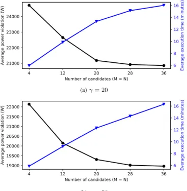
We define the power violation between an IT profile and a PW profile is the cumulative amount of power over these two profiles, that the IT power exceeds the PW power. In Fig 7, we show the average power violation and execution time in the same graphs. The two sub-figures correspond to two values of γ, γ = 20 and γ = 50. Similar to profile distance in Fig. 6, the power violation in both sub-figures (black curves) reduces when the number of candidates increases. However,
1 2 3 4 5 6 7 8 9 10111213141516171819202122232425262728 Round 1.0 1.2 1.4 1.6 1.8 2.0 Distance Distance 1 2 3 4 5 6 7 8 9 10111213141516171819202122232425262728 Round 1.0 1.2 1.4 1.6 1.8 2.0 Distance Distance 1 2 3 4 5 6 7 8 9 10111213141516171819202122232425262728 Round 1.0 1.2 1.4 1.6 1.8 2.0 Distance Distance 1 2 3 4 5 6 7 8 9 10 11 12 13 14 15 16 17 18 19 20 21 22 23 24 25 26 27 28 29 Round 500 1000 1500 2000 2500 3000 3500 0 500 1000 1500 2000 2500 ITDM PDM Po w e r (W ) Distance 1 2 3 4 5 6 7 8 9 10111213141516171819202122232425262728 Round 1.0 1.2 1.4 1.6 1.8 2.0 Profile Distance Distance 1 2 3 4 5 6 7 8 9 10111213141516171819202122232425262728 Round 1.0 1.2 1.4 1.6 1.8 2.0 Power (W) Distance
Fig. 4: Power level and distance over negotiation round
1 2 3 4 5 6 7 8 9 10 11 12 13 14 15 16 17 18 Round 1.2 1.4 1.6 1.8 2.0 2.2 2.4 Profile Distance = 20 = 50 = 100
Fig. 5: Profile distance over negotiation round
20 35 50 65 80 1.5 2.0 2.5 3.0 3.5
Average profile distance
M = N = 4 M = N = 12 M = N = 20 M = N = 28 M = N = 36
Fig. 6: Average profile distance over γ
the execution time (blue curves) grows with the number of candidates. Note that we run the negotiation algorithm on a local computer with an Intel ®processor of 4 cores 2.20GHz, and 8.27GB memory. When running the algorithm with other computing capacity, the execution time will vary.
In Table. II, we compare GAN with two other ap-proaches, namely scheduling-based negotiation (SAN) and GreenSlot [8]. SAN is our another proposed algorithm for ne-gotiation. In this algorithm, the two sub-systems are treated as black-boxes. Each sub-system proposes its preferred profiles, called hints, and exchanges with the other system. A
sub-system proposes its hints by selecting from a set of candidates, with regard to the hints of the other sub-system. Specifically, a sub-system grades each of its candidate based on the weighted sum of utility and the distance between that candidate and the hints of other sub-system. Then the candidates are sorted, and the top candidates are selected. At the next round, the scheduler of each sub-system replaces the selected profiles with newly proposed profiles. The two sub-systems repeat the process until the two sets of hints closely match each other.
We implemented the "GreenVarPrices" version of GreenSlot with some modifications and simplifications. We modify to have GreenSlot use similar workload and machine model with our setup. The important changes are (i) the renewable energies can be foretasted deterministically, (ii) the time of job running is preset, (iii) a job that was due is also scheduled, and (iv) multiple jobs can be run concurrently by a machine. Table. II provides the comparisons on average executing time (Avg. exe. time), profile distance (Avg. prof. dist.), utility (Avg. util.), and total utility (Tot. util.). The utility of GreenSlot and SAN are computed by calling the GAN’s procedures that compute utility. The total utility in the fifth column is the sum of utilities in the forth column. We define the same stopping criteria by setting the distance threshold ε = 1.2. With SAN and GAN, we present two scenarios with two values of M and N , i.e., M = N = 20 and M = N = 36. In general, GAN has the highest performance in profile distance and utility, although its execution time is higher than the others. Note that GreenSlot has significantly lower execution time than the other because this algorithm does not require an iterative negotiation process. Moreover, GreenSlot’s profile distance is not showed because there are not two separate sub-systems in this algorithm.
In terms of utility, compared to GreenSlot and GAN, the SAN’s PWS utility is especially lower than its ITS utility because SAN focuses on IT scheduling. In addition, SAN ob-tains lower total utility than GAN, which can be explained by the fact that SAN’s algorithm has higher degree of heuristics. Moreover, the selection criteria in SAN’s algorithm depends directly on the profile distance, which compromises between utility and distance; while in GAN, the profile distance mostly affects only stopping criteria. The total utility of GAN is also significantly higher than GreenSlot because the main objective of GreenSlot is to maximize the green energy consumption, so that the utility is not taken into account. As a result, only after the GreenSlot algorithm outputs final profiles, we can call the GAN’s procedures to compute utility for those profiles.
VII. CONCLUSIONS
We study the management of the electrical and IT infras-tructure in a datacenters completely operated under renewable sources. The objective is to reach a solution that compromises efficiently between energy supply and demand, taking into account the sub-systems’ constraints. A game-based algorithm is proposed to allow negotiating between ITS and PWS. The information about negotiation direction is exchanged between two sub-systems, under the model of buying-supplying. The
4 12 20 28 36 Number of candidates (M = N) 21000 22000 23000 24000
Average power violation (W) 6
8 10 12 14 16
Everage execution time (minutes)
(a) γ = 20 4 12 20 28 36 Number of candidates (M = N) 19000 19500 20000 20500 21000 21500 22000
Average power violation (W) 6
8 10 12 14 16
Everage execution time (minutes)
(b) γ = 50
Fig. 7: Average power violation and execution time.
Setup Avg. exe. time (min) Avg. prof. dist. Avg. util. (ITS, PWS) (Euro) Tot. util. (Euro) GreenSlot 0.43 (67.67, 46.30) 113.97 SAN M = N = 20 6.08 1.20 (67.77, 40.29) 108.06 GAN M = N = 20 6.80 1.17 (150.95, 106.67) 257.62 SAN M = N = 36 9.49 1.18 (103.20, 55.40) 158.6 GAN M = N = 36 10.69 1.17 (185.88, 125.92) 311.8
TABLE II: Summarized performance of three approaches experiments show that the proposed negotiation provides sta-ble solutions, and outperforms other approaches on utility and QoS. These are promising results in terms of applicability since the number of iterations required for convergence is in the order of tens. Moreover, the resulted power profile is at the time scale of 72 hours, which means that after running tens of iterations, we obtain the solution for 3 days of datacenter’s operation. We plan, as future research, to investigate a multi-time scale model for GAN, allowing the algorithm reach short-term solutions for small time-scale events, at the same time keeping long-term objectives. This model is needed for the systems that include multiple sub-systems and involve various time scales.
REFERENCES
[1] M. Avgerinou, P. Bertoldi, and L. Castellazzi, “Trends in data centre energy consumption under the european code of conduct for data centre energy efficiency,” Energies, vol. 10, no. 10, p. 1470, 2017.
[2] J. Popovi´c-Gerber, J. A. Oliver, N. Cordero, T. Harder, J. A. Cobos, M. Hayes, S. C. O’Mathuna, and E. Prem, “Power electronics enabling efficient energy usage: Energy savings potential and technological chal-lenges,” IEEE transactions on power electronics, vol. 27, no. 5, pp. 2338–2353, 2012.
[3] A. H. Khalaj, K. Abdulla, and S. K. Halgamuge, “Towards the stand-alone operation of data centers with free cooling and optimally sized hybrid renewable power generation and energy storage,” Renewable and Sustainable Energy Reviews, vol. 93, pp. 451–472, 2018.
[4] M. Haddad, J. M. Nicod, C. Varnier, and M.-C. Peéra, “Mixed in-teger linear programming approach to optimize the hybrid renewable energy system management for supplying a stand-alone data center,” in 2019 Tenth International Green and Sustainable Computing Conference (IGSC). IEEE, 2019, pp. 1–8.
[5] L. Liu, C. Li, H. Sun, Y. Hu, J. Gu, T. Li, J. Xin, and N. Zheng, “Heb: deploying and managing hybrid energy buffers for improving datacenter efficiency and economy,” in ACM SIGARCH Computer Architecture News, vol. 43. ACM, 2015, pp. 463–475.
[6] I. Goiri, M. E. Haque, K. Le, R. Beauchea, T. D. Nguyen, J. Guitart, J. Torres, and R. Bianchini, “Matching renewable energy supply and demand in green datacenters,” Ad Hoc Networks, vol. 25, pp. 520 – 534, 2015.
[7] C.-M. Wu, R.-S. Chang, and H.-Y. Chan, “A green energy-efficient scheduling algorithm using the dvfs technique for cloud datacenters,” Future Generation Computer Systems, vol. 37, pp. 141–147, 2014. [8] Í. Goiri, K. Le, M. E. Haque, R. Beauchea, T. D. Nguyen, J. Guitart,
J. Torres, and R. Bianchini, “Greenslot: scheduling energy consumption in green datacenters,” in Proceedings of 2011 International Conference for High Performance Computing, Networking, Storage and Analysis, 2011, pp. 1–11.
[9] Í. Goiri, W. Katsak, K. Le, T. D. Nguyen, and R. Bianchini, “Parasol and greenswitch: Managing datacenters powered by renewable energy,” ACM SIGARCH Computer Architecture News, vol. 41, no. 1, pp. 51–64, 2013.
[10] I. De Courchelle, T. Guérout, G. Da Costa, T. Monteil, and Y. Labit, “Green energy efficient scheduling management,” Simulation Modelling Practice and Theory, vol. 93, pp. 208–232, 2019.
[11] Y. Li, A. C. Orgerie, and J. M. Menaud, “Balancing the use of batteries and opportunistic scheduling policies for maximizing renewable energy consumption in a cloud data center,” in 2017 25th Euromicro International Conference on Parallel, Distributed and Network-based Processing (PDP), March 2017, pp. 408–415.
[12] J. Pierson, G. Baudic, S. Caux, B. Celik, G. Da Costa, L. Grange, M. Haddad, J. Lecuivre, J. Nicod, L. Philippe, V. Rehn-Sonigo, R. Roche, G. Rostirolla, A. Sayah, P. Stolf, M. Thi, and C. Varnier, “Datazero: Datacenter with zero emission and robust management using renewable energy,” IEEE Access, vol. 7, pp. 103 209–103 230, 2019. [13] S. Caux, P. Renaud-Goud, G. Rostirolla, and P. Stolf, “It optimization for
datacenters under renewable power constraint,” in European Conference on Parallel Processing. Springer, 2018, pp. 339–351.
[14] L. Grange, G. Da Costa, and P. Stolf, “Green it scheduling for data center powered with renewable energy,” Future Generation Computer Systems, vol. 86, pp. 99–120, 2018.
[15] M. Haddad, M.-C. Pera, and C. Varnier, “Stand-Alone Renewable Power System Scheduling for a Green Data-Center using Integer Linear Programming Version 1,” FEMTO-ST, Research Report, Mar. 2019. [Online]. Available: https://hal.archives-ouvertes.fr/hal-02081951 [16] M.-T. Thi, J.-M. Pierson, G. Da Costa, P. Stolf, J.-M. Nicod, G.
Ros-tirolla, and M. Haddad, “Negotiation game for joint it and energy man-agement in green datacenters,” Future Generation Computer Systems, vol. 110, pp. 1116–1138, 2020.
[17] M. R. Berthold and F. Höppner, “On clustering time series us-ing euclidean distance and pearson correlation,” arXiv preprint arXiv:1601.02213, 2016.
[18] D. R. Krause, R. Terpend, and K. J. Petersen, “Bargaining stances and outcomes in buyer–seller negotiations: experimental results,” Journal of Supply Chain Management, vol. 42, no. 3, pp. 4–15, 2006.
[19] D. G. Pruitt, “Bargaining behavior,” New York: Ac, 1981.
[20] J. L. Graham, “The problem-solving approach to negotiations in in-dustrial marketing,” Journal of Business Research, vol. 14, no. 6, pp. 549–566, 1986.
[21] R. J. Lewicki, D. M. Saunders, J. W. Minton, J. Roy, and N. Lewicki, Essentials of negotiation. McGraw-Hill/Irwin Boston, MA, 2011. [22] K. Kurowski, A. Oleksiak, W. Piatek, T. Piontek, A. Przybyszewski,
and J. Weglarz, “DCworms – A tool for simulation of energy efficiency in distributed computing infrastructures,” Simulation Modelling Practice and Theory, vol. 39, pp. 135–151, 2013.