Computational Design for the Next Manufacturing
Revolution
by
Adriana Schulz
Submitted to the Department of Electrical Engineering and Computer Science
in partial fulfillment of the requirements for the degree of
Doctor of Philosophy in Computer Science and Engineering
at the
MASSACHUSETTS INSTITUTE OF TECHNOLOGY
June 2018
c
○
Massachusetts Institute of Technology 2018. All rights reserved.
Author . . . .
Department of Electrical Engineering and Computer Science
May 22, 2018
Certified by. . . .
Wojciech Matusik
Associate Professor of Electrical Engineering and Computer Science
Thesis Supervisor
Accepted by . . . .
Leslie A. Kolodziejski
Professor of Electrical Engineering and Computer Science
Chair, Department Committee on Graduate Students
To my great-grandmother, who dreamt about an academic life. To my parents, who empowered me to live it.
Computational Design for the Next Manufacturing Revolution
by
Adriana Schulz
Submitted to the Department of Electrical Engineering and Computer Science on May 22, 2018, in partial fulfillment of the
requirements for the degree of
Doctor of Philosophy in Computer Science and Engineering
Abstract
Over the next few decades, we are going to transition to a new economy where highly com-plex, customizable products are manufactured on demand by flexible robotic systems. In many fields, this shift has already begun. 3D printers are revolutionizing production of metal parts in the aerospace, automotive, and medical industries. Whole-garment knitting machines allow automated production of complex apparel and shoes. Manufacturing elec-tronics on flexible substrates makes it possible to build a whole new range of products for consumer electronics and medical diagnostics. Collaborative robots, such as Baxter from Rethink Robotics, allow flexible and automated assembly of complex objects. Overall, these new machines enable batch-one manufacturing of products that have unprecedented com-plexity.
In this thesis, I argue that the field of computational design is essential for the next revo-lution in manufacturing. To build increasingly functional, complex and integrated products, we need to create design tools that allow their users to efficiently explore high-dimensional design spaces by optimizing over a set of performance objectives that can be measured only by expensive computations. In this work discuss how to overcome these challenges by 1) developing data-driven methods for efficient exploration of these large spaces and 2) performance-driven algorithms for automated design optimization based on high-level func-tional specifications. I showcase how these two concepts are applied by developing new systems for designing robots, drones, and furniture.
Thesis Supervisor: Wojciech Matusik
Acknowledgments
First and foremost, I would like to thank my PhD advisor, Wojciech Matusik, for his many teachings on conducting research: from picking good problems to framing and presenting ideas, and all that takes place in between. Wojciech always ensured I was granted exposure to the important tools and means that would help me grow into a successful researcher. Most of all, I thank him for encouraging me to dare to do things I would never have known I was capable of. This was only possible because he challenged me and made it safe for me to try. I would also like to thank my other committee members, Daniela Rus and Eitan Grinspun, for their teachings and mentoring. I thank Eitan for nurturing my interest in geometry, for teaching me how to defend my ideas so that I could better understand what makes a research problem interesting, and for all the wonderful advice over hummus at Columbia Hillel. I thank Daniela for introducing me to the amazing field of robotics, for showing me how to bring together ideas from different fields, and for always encouraging me to âĂIJkeep the gradient!”.
I would also like to thank the wonderful collaborators without whom this work would not be possible: Ariel Shamir, Justin Solomon, Ilya Baran, David Levin, Pitchaya Sitthi-amorn, Changxi Zheng, Bo Zhu, Andrew Spielberg, Tao Du, Jie Xu, Jeffrey Lipton, and Bernd Bickel. I am extremely grateful not only for the ideas and work they have contributed to this thesis, but also for the fun memories we created—especially during the weeks leading up to the Siggraph deadlines! I also thank the brilliant students I had the pleasure to supervise and who greatly contributed to this work: Wei Zhao, Harrison Wang, Robin Cheng, Baker Logan, Keneth Pinera, Luis Trueba, Katie Bartel, Nilu Zhao, Saul Lopez, Jackson Wirekoh, Molly Donalson, Helena Wang, Kendall Helbert, Alexxis Isaac, Isaque Dutra, Megan Chao, Diane Rosales, Marie Moudio, Brian Saavedra, and Emily Salvador.
I would like to thank the rest of the MIT faculty, students, and staff who provided great feedback, support, and friendship during this process. I thank David Karger, Fredo Durand, Solar-Lezama, Sylvain Paris, Boris Katz, and Charles K. Smart for the helpful ideas and discussions. I thank all the students from the MIT Graphics Group—especially Valentina Shin, James Minor, Desai Chen, Abe Davis, Javier Ramos, Michael Foshey, and Nick Bandeira—as well as the students at MIT DRL and Columbia Computer Graphics Group. I thank Bryt Bradley for being an incredible supporter over all these years.
I also want to thank the wonderful friends I made during the last few years as I was pursuing this degree. They made this process fun, made the hard moments better, and inspired me and changed me in more ways than I can describe. It would be impossible to name them all, but I’d like to especially thank Josh Pfeffer (without whose support I cannot imagine having submitted half of my papers), Natalie Mashian Fisher, and Luis Voloch.
Next, I would like to acknowledge and thank my mentors from my undergraduate and Masters studies in Brazil, Luiz Velho and Eduardo da Silva. Though they were not directly involved with the work in this thesis, they were fundamental in preparing me for it. I am very grateful for their teaching, mentorship, and support during my initial ventures in the academic world.
Last but not least, I want to thank my family. I thank my parents, Sonia and Mauro Schulz, who always nurtured my curiosity, who empowered me to come to MIT, and who supported me in every step of the way. I thank them for their constant love, closeness,
and for sending me far away so that I could pursue my own dreams. I know how hard that was and still is. I thank them for their contagious passion for academia, for being amazing role models, and for always pushing me to go a step beyond. I thank my mom for the long philosophical conversations, for introducing me to art and design, and for always challenging me to think deeply and outside the box. I thank my dad for inspiring my love for mathematics and for encouraging me to study Engineering, all the while pointing out to me how limited logic actually is. Finally, I thank my sister, Lilian Schulz, my lifelong best friend. My sister was always there to help me out—from my homework in grade school to my faculty applications—and none of my achievements would have been half as fun if she had not been there to celebrate them with me!
A Story Before We Start
In contrast to the rest of this thesis, where I have verified all the finding to the best of my abilities, this story may not be entirely true. But I will take the liberty to share it, because there is something personal about a thesis that makes it different from my list of published papers. If this work is supposed to summarize what I have discovered during my PhD, then this story, however accurate or inaccurate it may be, is essential to making this work complete.
They say Rousseau loved the opera so much that he would visit this specific opera house once every week. And he would sit in the back listening to the women’s voices—such mar-velous, enchanting voices, that he would imagine them to be the most beautiful women in the world. One day, a friend, aware of his adoration, agreed to arrange for him to have dinner with the singers one evening after the show.
On the day the dinner was scheduled, Rousseau came to the opera house delighted. He sat that night in his usual seat in the back, completely captivated by the singers and waiting in anticipation to meet the women to whom such voices belonged. But as he joined the dinner party he was surprised to see women who were very far from the beauty standards he envisioned. Most of the women had birth deformities or had suffered physical traumas that had left them disfigured. Because of their unattractive exterior, they had been taken care of by an orphanage that sheltered them and educated them to pursue a career where only their voices could be heard. Rousseau was so surprised, it took him a moment to gather himself and join the party. But the women were sweet and cheerful, so the dinner was pleasant and Rousseau came home content.
A week passed by and once again Rousseau made his way to the opera house. From his usual seat in the back he heard the women’s voices. They were as graceful and dazzling as they has always been. He closed his eyes and imaged how women who possessed such voices looked. He quickly realized he had seen their faces a week before. But as he sat and heard their voices, their angelic, bewitching voices, he imaged them to be the most beautiful women in the world.
The person who started this PhD, imagined academia to be “the most beautiful place in the world.” An open invitation to push even if ever so slightly the invisible wall that surrounds us—the frontier of human knowledge. The one who writes this thesis has seen academia in a much brighter light. There were surprises that were not particularly pleasant. There were times I needed a few moments to “gather myself.” But I can still see that invisible wall and now I am surrounded by incredible friends and mentors who are actively pushing it. It has been a privilege to witness their work, their intellectual integrity, their passion, their bad hair days. Academia enchants me today even more than it ever did.
The main discovery of my PhD was this imperfect yet amazing world, which I hope to always be a part of.
Contents
1 Introduction 29
1.1 The Next-Manufacturing Revolution . . . 29
1.2 Abstraction of Design for Manufacturing . . . 30
1.3 Approach and Contributions . . . 32
1.3.1 Data-Driven Methods . . . 32
1.3.2 Performance-Driven Search Methods . . . 33
1.3.3 End-to-End Systems . . . 34 1.4 Thesis Overview . . . 35 1.5 Contributions . . . 35 2 Related Work 37 2.1 Data-Driven Methods . . . 37 2.1.1 Parametric Modeling . . . 38 2.1.2 Parametric CAD . . . 38 2.2 Performance-Driven Methods . . . 40 2.2.1 Interactive Exploration . . . 40 2.2.2 Optimization . . . 40
3 A Collection of Manufacturable Designs 43 3.1 Introduction . . . 43
3.2 Manufacturable Designs . . . 43
3.2.1 Items Catalog . . . 43
3.2.2 Set of Designs . . . 44
3.3 Parametric Manufacturable Designs . . . 45
3.4 Automatic Hierarchical Parametrization . . . 45
3.5 Defining the mapping function 𝐹 . . . 46
3.5.1 Geosemantic Relationships . . . 47
3.6 Connections . . . 49
3.7 Discussion . . . 50
4 Retrieval on Collections of Manufacturable Designs 51 4.1 Introduction . . . 51
4.2 Related Work . . . 53
4.3 Representation of Parametric Shapes . . . 55
4.4 Algorithm . . . 57 4.4.1 Unbounded Manifolds . . . 58 4.4.2 Bounded Manifolds . . . 60 4.5 Retrieval . . . 62 4.6 Experimental Setup . . . 63 4.6.1 Database . . . 63 4.6.2 Descriptors . . . 64 4.7 Evaluation . . . 65 4.7.1 Manifold Representation . . . 65 4.7.2 Retrieval . . . 69 4.7.3 Limitations . . . 73 4.8 Discussion . . . 75
5 Assembly-Based Design for Manufacturing 77 5.1 Introduction . . . 77 5.2 Design Workflow . . . 78 5.3 Parametric Manipulations . . . 79 5.4 Composition . . . 81 5.5 Snapping . . . 81 5.6 Connecting . . . 83
5.6.1 Searching for Connections . . . 83
5.6.2 Final Composition . . . 84
5.7 Results . . . 85
5.7.1 Modeling . . . 85
5.7.2 Fabrication . . . 86
5.8 Discussion . . . 86
6 Interactive Design-Space Exploration 89 6.1 Introduction . . . 89
6.2 Related Work . . . 90
6.3 Workflow . . . 91
6.4 Precomputation Overview and Notations . . . 91
6.4.1 Refinement Relations . . . 93
6.4.2 Adaptive Sampling . . . 94
6.4.3 Refinement Notations . . . 94
6.5 Adaptive Refinement Strategy . . . 95
6.5.1 Motivation . . . 95
6.5.2 Algorithm . . . 98
6.5.3 Extension to Cubic B-splines . . . 101
6.6 Homeomorphic Mapping . . . 103
6.6.1 Motivation . . . 103
6.6.2 Algorithm . . . 104
6.7 Results . . . 107
6.7.1 Application in Shape Optimization . . . 110
6.8 Discussion . . . 112
7 Interactive Performance-Space Exploration 113 7.1 Introduction . . . 113 7.2 Related Work . . . 114 7.3 Mathematical Preliminaries . . . 115 7.3.1 Definitions . . . 115 7.3.2 KKT Conditions . . . 116 7.4 First-Order Approximation . . . 117
7.5 Pareto Front Discovery . . . 118
7.5.1 Data Structure . . . 118 7.5.2 Discovery Algorithm . . . 119 7.5.3 First-Order Approximation . . . 121 7.5.4 Sparse Approximation . . . 122 7.5.5 Visualization . . . 123 7.6 Results . . . 123 7.6.1 Experiments . . . 124 7.6.2 Design Applications . . . 128 7.7 Discussion . . . 131 8 Applications 133 8.1 Introduction . . . 133
8.2 Interactive Design of Ground Robots . . . 134
8.2.1 System Overview . . . 134
8.2.2 Methods Overview . . . 136
8.2.3 Results . . . 138
8.3 Interactive Multicopter Design . . . 142
8.3.1 System Overview . . . 142 8.3.2 Methods Overview . . . 142 8.3.3 Results . . . 143 8.4 Robot-Assisted Carpentry . . . 145 8.4.1 Systems Overview . . . 146 8.4.2 Methods Overview . . . 146 8.4.3 Results . . . 148 9 Conclusion 151 9.1 Future Work . . . 151 9.1.1 Data-Driven Methods . . . 152 9.1.2 Performance-Driven Methods . . . 153 9.1.3 End-to-End Systems . . . 155 9.2 Lessons Learned . . . 156
A Proofs of Interpolation Algorithm 157
A.1 Notation . . . 157
A.2 Properties of Step 2 . . . 157
A.3 Local Point Lemma . . . 158
A.4 Locality proof with Linear Precision . . . 159
A.4.1 Preservation over Basis Refinement . . . 159
A.4.2 Preservation over Element Refinement . . . 160
A.5 Example . . . 164 B Proof of the First-Order Approximation of the Pareto Front 167
List of Figures
1-1 The next manufacturing revolution. In a very near future, we will have work-shops where automated manufacturing machines will make customized, com-plex, multi-material parts and collaborative robots will allow flexible and au-tomatic assembly of objects that have multiple functionalities. . . 30 1-2 Designing a robot means selecting a point in a high-dimensional design space
that includes specification of the robot’s geometry, electronic components, and control software. Users select this point based on how it is mapped to a performance space, which defines important metrics that designers take into account when optimizing the models (e.g., the trajectory, fabrication cost, and reaction to an external force). . . 31 1-3 An example of a parametric design. The original design is shown in gray, and
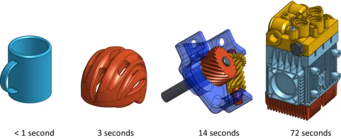
the new designs generated by varying the parameters are shown in yellow. . 33 1-4 We apply data-driven and performance-driven algorithms to develop
inter-active systems for design of complex functional mechanisms. From left to right: a data-driven method that automatically handles manufacturing de-tails and guarantees [Schulz et al., 2014]; real-time performance exploration and optimization for functionality-driven design [Schulz et al., 2017c]; end-to-end system for design and manufacturing of ground robots that allows for concurrent design of both geometry and motion [Schulz et al., 2017b]. . . . 34 2-1 When engineers design shapes, they embed their experience and knowledge
in carefully selected, fabrication-aware parameters such as this fillet radius, which encapsulates a curved transition along an edge, and this chamfer dis-tance, which describes the slope transition between two surfaces. These in-clude fabrication limitations that take into account the different processes. This example includes minimum radius constraints on internal cuts for com-patibility with milling machines. . . 39 2-2 Regeneration times for parameter changes using Onshape for models with
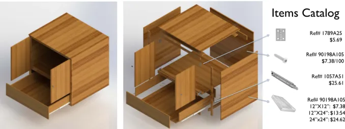
increasing level of complexity. . . 40 3-1 An example of a fabricable object from our collection (left). Each design is
detailed down to the level of individual screws, and each part maintains a reference to the items used from the items catalog (right). . . 44
3-2 From left to right: a design example of a toy wagon, the hierarchical tree, and a visualization of the connections. The arrow on the handle indicates that this part has an articulation, namely that it can rotate along the depicted axis. The tree includes the geosemantic relationships that are stored at each level of the hierarchy, 𝐶0 to 𝐶4 (shown in blue), as well as connections (depicted in
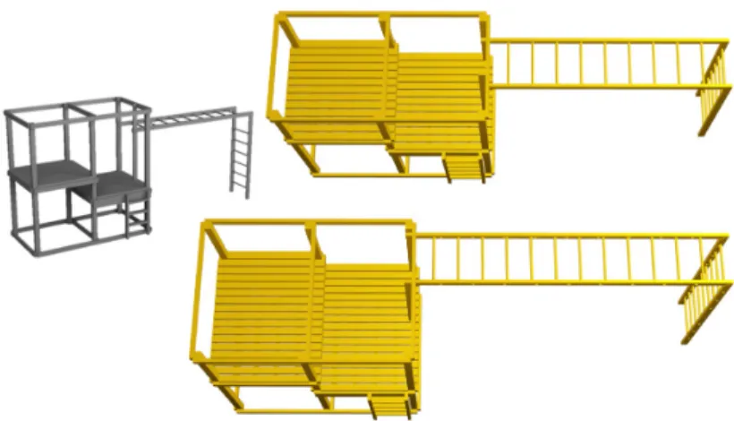
red). The visualization on the right illustrates the information contained in each connection node. . . 46 3-3 A parametric model with pattern elements. Upon resizing, both the number
of floor planks and the number of rungs in the monkey bars change. . . 47 3-4 We show a simple 2D table consisting of three parts, a top and two legs (Leg1
and Leg2). Each part is contained within a single element for which the q𝑖
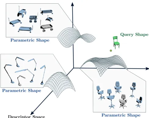
are the positions (𝑥, 𝑦) and sizes (∆𝑥, ∆𝑦) of the bounding box of the part. . 48 4-1 We propose a method for shape retrieval from parametric shape collections
that uses a descriptor space representation. While shape descriptors map sin-gle shapes to points in a descriptor space, smooth descriptors map parametric shapes to low dimensional manifolds in this space. Our method efficiently represents these manifolds in order to allow for accurate and fast retrieval of the closest parametric model to a given query shape. . . 52 4-2 The function ℳ(𝑞) = (𝒟 ∘ ℱ)(𝑞) is a composition of the mapping function
ℱ from parameter values to a geometry with the signature function 𝒟 which generates a descriptor for a given geometry. . . 56 4-3 The coverage of a point (left) and of a tangent line (right) are defined by the
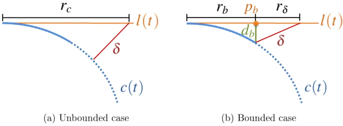
region of the manifold (here illustrated as a curve 𝑐(𝑡)) that is well approxi-mated by this primitive given the allowed approximation error 𝛿. While the coverage of the point 𝑐(0) is directly proportional to 𝛿, the coverage of the tangent line 𝑙(𝑡) is proportional to 𝑑, which depends on the curvature. . . 58 4-4 Computation of the bounding radius for a tangent space primitive 𝑙(𝑡) on
the manifold 𝑐(𝑡). In the illustration, the dotted line represents the part outside the boundary of the manifold and 𝛿 is the allowed approximation error. Left: when we do not take the boundary into account the bounding radius is determined uniquely by the curvature constraint 𝑟𝑐. Right: when we
are close to the boundary, the radius is computed as 𝑟𝑏 +𝑟𝛿, where 𝑟𝑏 is the
distance to the boundary and 𝑟𝛿 is the amount by which we can expand the
radius preserving tightness constraints. We can compute 𝑟𝛿 from 𝛿 and 𝑑𝑏,
which is the distance from the boundary point 𝑝𝑏 on 𝑙(𝑡) to the manifold. . . 60
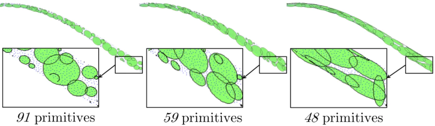
4-5 From left to right: covering the manifold with tangent spaces bounded by hyperspheres, non-oriented ellipsoids, and oriented ellipsoids. This example illustrates that the number of primitives needed to represent the manifold for the same value of 𝛿 is reduced when we use better primitives. We notice that even in this example with a 2-dimensional parameter space there is a signifi-cant improvement when oriented primitives are used. The blue dots represent the underlying manifold represented via super sampling. (Please note that these are high dimensional primitives projected to 2D for visualization and therefore appear slightly distorted.) . . . 62
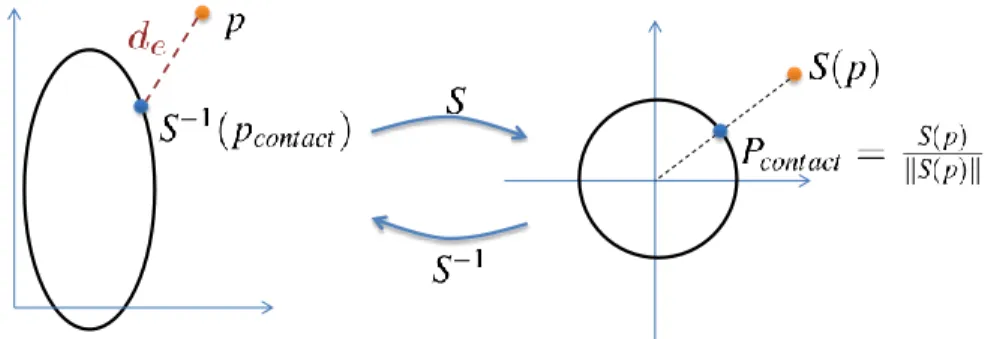
4-6 Approximating the distance 𝑑𝑒 from the projected point 𝑝 to the hyperellipse.
Let 𝑆 be a scaling function that maps the hyperellipse to the unit hypersphere centered at the origin. The point on the hypersphere that is the closest to 𝑆(𝑝) is given by 𝑝𝑐𝑜𝑛𝑡𝑎𝑐𝑡= ‖𝑆(𝑝)‖𝑆(𝑝) . We use the inverse mapping and approximate the
distance from 𝑝 to the hyperellipse as 𝑑𝑒≈ ‖𝑝 − 𝑆−1(𝑝𝑐𝑜𝑛𝑡𝑎𝑐𝑡)‖. . . 63
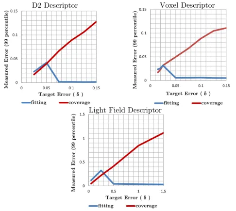
4-7 Comparison between adaptive sampling and rejection sampling on a simple paraboloid example. Our rejection sampling scheme was done for both point and planes for a fixed approximation error 𝛿. The number of samples for the adaptive sampling schemes was chosen to be the same as the result of the rejection sampling for both points and planes. The top row shows the results for point samples. Though both methods return a uniform distribution, in the adaptive sampling scheme points tend to clump together and leave gaps. The bottom row results for approximating with tangent spaces (we only display the center of the tangent space for simplification). Once again both methods display the desired distribution (based on curvature) and rejection sampling covers the space more effectively. . . 66 4-8 Measuring fitting and coverage errors as a function of the target parameter
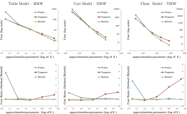
𝛿 for the implemented descriptors. we observe that both measured errors are within the bounds of 𝛿. For large values of 𝛿 we observe that the fitting error drops to zero. This is because for very coarse approximations, our algorithm prefers points to tangents – the coverage of points become larger with 𝛿, while plane coverage is still limited by the curvature and the boundary of the manifold. Since absolute distance values depend on descriptors (and are much larger for the Light Field descriptor), the ranges of the target errors for this experiment were chosen so that the number of samples were similar for all descriptors. . . 67 4-9 Comparison between our hybrid method and using a single primitive. Top row:
shows the storage cost of each representation across different target parameters 𝛿 in log scale. Bottom row: the relative cost of the single primitive methods while compared to our method. . . 68 4-10 Demonstration of query failures when representation only consists of the mean
shape. From left to right: the mean shape of some parametric models in the database, query shape given by a random parameter setting of each parametric model, and the closest mean shape retrieved from the database. Since changes in parameter settings significantly alter the geometry, the closest mean shapes are usually not from the parametric models that originate the queries. . . . 70 4-11 Comparison between our approach and the naive one. We measure the
dif-ference between the distance to the closest primitive in the collection and the distance to the correct manifold and show the worst case for both approaches for querying points sampled on the full database and on individual categories. From these results we verify that our method has a better performance across all categories. . . 71
4-12 Results of retrieval. From left to right: query shape, result for D2 descriptor (for increasing target errors), and result for Voxel descriptor (for increasing target errors) and results for the Light Fied descriptor (for increasing target errors). . . 71 4-13 Precision-recall plots evaluating classification accuracy for our method
com-pared to using only mean shapes for different descriptors. . . 73 4-14 Comparison of retrieval with mean shapes only and manifold representation
for the Light Field descriptor. From left to right: query shape (green), closest mean shape retrieved (gray), closest parametric shape retrieved with param-eter fitting (blue) with its corresponding mean shape (gray). We observe that using the parametric shapes we retrieve models that are more similar in geometry but may lie on a different class. . . 74 5-1 The design and fabrication by example pipeline: casual users design new
models by composing parts from a database of parametric manufacturable designs. The system assists the users in this task by automatically aligning parts and assigning appropriate connectors. The output of the system is a detailed model that includes all components necessary for fabrication. . . 77 5-2 The user interface. Icons that link to components of the database are displayed
on the left, and the modeling canvas is on the right. . . 79 5-3 An illustration of how parametric variations can be explored in our tool. The
arrows control translation, while spheres control scaling. On the left, we show the controls on a leaf node of the hierarchy; on the right, we show the controls on an internal node. During manipulation, elements on the selected node are represented in full color, while the others become semi-transparent. Notice that constrained degrees of freedom are hidden. For example, the user is unable to change the thickness of the shelf, since the items catalog states that planks of wood can be cut only in two directions. . . 80 5-4 An example of snapping to constraints. We add a tabletop 𝑇𝐴to the working
model 𝑇𝑊 containing eight legs (right). The coplanarity constraints on the
original design 𝑇𝐷 that contained 𝑇𝐴 are represented by the normals of the
corresponding planes (left; we show only the vertical ones). The feasible snapping configurations for q𝐴are shown on the right. The system will choose
one of these configurations: its choice will depend on the scale parameters and the position on which the user places the tabletop. . . 82 5-5 An illustration of snapping for functional objects. When a door is added to
the side of a cabinet, it automaticaly rescales so that, when shut, it will align with the oposite side. At left, a door is added to the working model. From left to right: the added door before snapping, the snapped configuration, and a visualization of the snapped configuration when the door is closed. The rotation axis of the articulations is depicted by the arrows. . . 83
5-6 An example of changing parameters to fit connectors. From left to right: the bottom shelf snapped to the bottom of the table, the resulting configuration of the model after the connecting step, and the vizualization of the connec-tors (principal elements are made semi-transparent). Notice that, in order to connect the bottom shelf to the table legs, the system raises the shelf above the ground to leave room for l-brackets. . . 85 5-7 Examples of models designed using our system and the number of individual
parts they comprise. Different colors indicate the different parts that were added to the model. . . 85 5-8 An example of different manipulations of a working model after it has been
composed from multiple parametric designs. . . 86 5-9 From left to right: input designs, models created using the system, and
fab-ricated results. We highlight the connecting elements on the first model by making all principal elements semi-transparent. . . 87 6-1 Our method takes as input a CAD model with a set of exposed parameters
which define the design space. We sample the parametric space in an adaptive grid and propose techniques to smoothly interpolate this data. We show how this can be used to drive interactive exploration tools that allow designers to visualize the shape space while geometry and physical properties are updated in real time. . . 90 6-2 The neighborhood of an element, denoted ℬ(𝑒𝑙), is defined as the set of
adja-cent samples (left). The neighborhood of a sample, denoted 𝒩 (𝑥𝑘), is defined
as the set of adjacent elements (middle). We also extend the definition of 𝒩 (𝑥𝑘)to any point 𝑝 ∈ 𝒜 as the set of adjacent elements (right). . . 92
6-3 When locality is enforced, the number of consistent representations 𝑝𝑙 𝑘 that
are needed at each sample 𝑥𝑘 depends on the cardinality of 𝒩 (𝑥𝑘). . . 93
6-4 Refinement of linear B-splines. . . 93 6-5 A linear B-spline 𝜑𝑗
𝑖 is illustrated in blue: the blue "‘x"’ is the center and
the region where it assumes non-zero values is shaded in light blue. The local sample set of this linear B-spline ℒ(𝜑𝑗
𝑖), is defined as the set of samples 𝑥𝑘
such that 𝑆(𝜑𝑗
𝑖) ⊂ 𝒩 (𝑥𝑘)and is illustrated in black. . . 95
6-6 Comparison between multi-linear interpolation (left), where discontinuities appear along T-junctions, and our method (right), where the interpolation is continuous. . . 96 6-7 Our method of combining element refinement with basis refinement:
interpo-lated values inside each element only depend on the samples that lie on the boundary of that element. . . 96 6-8 Hierarchical and quasi-hierarchical basis refinement strategies. Both of these
schemes violate locality on element 𝑒1𝐴 since the basis function 𝜑01 does not
vanish on this element. The sample outside ℬ(𝑒1𝐴) affecting this element is
highlighted in red. . . 97 6-9 Example of samples added for a given split in 2D and 3D. Split element, split
6-10 Illustration of refinement in two dimensions. Letters are used to index 𝑥𝑘 for
clarity. When the element is split, new samples are added, the B-splines 𝜑𝑗 𝑖
are refined and the new basis functions 𝜓𝑗
𝑖 are recomputed to ensure locality. 100
6-11 The neighborhood 𝒩 (𝑥𝑘)of a sample 𝑥𝑘 (left) and the neighborhood ℬ(𝑒𝑙)of
an element 𝑒𝑙 (right) for cubic B-splines. . . 101
6-12 Refinement of cubic B-splines. . . 102 6-13 The mapping 𝐹 : 𝑝𝑙 𝑘 → 𝑝 𝑙 𝑘 is used to obtain 𝑝 𝑙 𝑘 for 𝑥𝑘 ∈ ℬ(𝑒𝑙) ∖ ℬ(𝑒𝑙). . . 103
6-14 Example of referencing in Onshape. The user applies a feature to a given face which is highlighted (left), and then changes parameter making other faces and edges of the model merge or split (right). Onshape’s referencing scheme guarantees that the feature will still be applied to the correct face even after these changes are made. . . 104 6-15 Two examples of a fillet feature applied to edges. After this feature is defined,
parameter changes on earlier features in the feature list split the edges into two parts. The way the edge references are handled in order to re-generate the fillet depends on the feature history, not the geometry. On the model on the left, the CAD system applies the fillet to both edges generated by the split; on the model on the right, the fillet is applied to only one of the edges. 105 6-16 Common patch layout given a source and target geometry. Top to bottom:
B-rep with highlighted topological changes, paths extracted from CAD, complete patch layout. . . 106 6-17 Mapping result. Given a source geometry and a target mesh topology the
mapping outputs a mesh with the source geometry and target topology. . . . 106 6-18 Examples of interactive visualization. On the left we show each model in red
boxes and the regions with fixed boundary conditions and forces with red arrows. On the right we show results from our visualization interface. As the user varying the parameters, geometry is updated is real time. The top four rows show pre-computed stress analysis. On the forth row the force direction also varies and is illustrated with a red arrow. The fifth row shows a result with fluid simulation. The last row shows a results with thermoelastic simulation where the colors display (from left to right) heat distribution, deformation and stress. . . 108 6-19 Result of shape optimization. Stress is minimized on an arbor press for two
different use cases, a tall one is shown on the right and a short one on the left. 111 7-1 Our method allows users to optimize designs based on a set of performance
metrics. Given a design space and a set of performance evaluation functions, our method automatically extracts the Pareto set—those design points with optimal trade-offs. We represent Pareto points in design and performance space with a set of corresponding manifolds (left). The Pareto-optimal so-lutions are then embedded to allow interactive exploration of performance trade-offs (right). The mapping from manifolds in performance space back to design space allows designers to explore performance trade-offs interactively while visualizing the corresponding geometry and gaining an understanding of a model’s underlying properties. . . 114
7-2 The Pareto set represents the points in design space with optimal performance trade-offs that get mapped to the Pareto front in performance space. Different colors indicate different manifolds in design and performance space with a one-to-one mapping. Any ray from the origin (blue line) can only intersect the Pareto front once. . . 115 7-3 The performance buffer: since a ray from the origin can only intersect one
point in the Pareto front, we use a buffer discretized by (hyper)spherical co-ordinates for storage. . . 119 7-4 A single iteration of the discovery algorithm: random samples x𝑖
𝑠are generated
from the current data on the buffer (illustrated in gray) and optimized for a search direction s(x𝑖
𝑠) (blue arrow). A first-order approximation around the
result of this optimization, x𝑖
𝑜, generates the corresponding manifolds in both
design and performance space (red lines) and the buffer is updated based on this new data. . . 120 7-5 Search directions for buffer cells for 𝑑 = 2. For diversity, different regions of
the performance space get assigned different search directions. We use the buffer discretization to define these directions as illustrated in the figure. . . 121 7-6 Nondominated solutions for various well-established benchmark problems
us-ing our proposed approach. Top two rows: Solutions for the five real-valued ZDT problems. Bottom row: Solutions for the first three DTLZ problems with three objectives. Our approach was able to converge to the ground truth Pareto front in all cases. . . 124 7-7 Results for Pareto front discovery on Fourier benchmark. The figure illustrates
how the Pareto front can be covered by a set of individually smooth regions which are mapped via 𝐹 from affine subspaces in the design space. Each corresponding pair in design and performance space is illustrated in a different color. In high-dimensional cases in design space, dimensionality-reduction via principal component analysis is applied for visualization purposes. . . 126 7-8 A direct piecewise-linear interpolation result of the example shown on the first
row of Figure 7-7. The optimal solution is chosen from the list of points at each buffer cell (blue points) and a denser sampling is generated by linearly interpolating the preimage of neighboring points in performance space (red points). Since the Pareto front is comprised of distinct manifolds, the linearly interpolated points have no guarantee of Pareto optimality. For illustrative purposes, the interpolation is performed on a sparse set of the discovered solutions. . . 127 7-9 Performance Space Assessment of the approximation error associated with
our first-order expansion method on the example shown on the first row of Figure 7-7. Left: plot in performance space of the discovered Pareto front (grey) and results of the same points after performing an additional local optimization (maroon). Right: histogram showing the approximation error for points on the discovered Pareto front. . . 127
7-10 First-order approximation for a point x on the Pareto front of the bi-objective Kursawe problem Kursawe [1991] (true front shown in black). The first-order approximation defined by our method (red) is compared to the mapping of affine spaces around x generated using directions chosen uniformly at random (gray). . . 128 7-11 Examples of CAD models processed using our proposed technique. From
left to right: Pareto-optimal points in design space (illustrated with multi-dimensional scaling via principal component analysis for models with more than three design parameters); Pareto-optimal points in performance space; the resulting embedding and illustrations of geometric results for some sam-pled points. Across all figures, the different colors correspond to different regions resulting from local expansion in design space. . . 129 7-12 Example of two variations of the brake hub that have similar performance
metrics but very different design parameters. Our system can expose these re-lationships providing intuition to designers about the structural nature of the model. The metrics are shown under a normalization for easy comparison— the Pareto front is rescaled to lie between zero and one. . . 130 7-13 Example of two different lamps (front and side view) that have the same
performance across all metrics. Due to the large dimensionality of the design space, these two configurations have the same stability, mass, and distance to the focal point. . . 131
8-1 A robot design that topples while walking (a) can be modified to follow a gait that only wobbles slightly (b), but changing the geometry (c) allows the robot to move much faster and more steadily. . . 134 8-2 System diagram. Users interact with geometry and gait design tools. The
designed models are simulated to provide feedback to the user. The user may iterate over the design before fabricating and assembling the model. . . 135 8-3 User interface. Icons that link to geometry components are displayed on the
left and the gait design tool is on the bottom. Users design models by dragging components into the center canvas and editing them. Performance metrics for the design are shown on the right. . . 135 8-4 Geometry components by category. Our system’s database contains 45
com-ponents: 12 bodies, 23 limbs, and 10 peripherals. . . 136 8-5 Joint controllers for each joint type. Controllers for every joint are separated
into a step phase (shown in green) and a reset phase (shown in red). Users modify gaits by changing the 𝜃𝑖 values for each joint and defining the step
8-6 One of the geometry components in the database, with both its 3D shape and 2D unfolding. The component has parameter values of diameter 𝑞𝑑 and width
𝑞𝑤. The 3D and 2D representations are coupled so that they are
simultane-ously updated as parameters are changed. In order to allow the assembly-based modeling to work with our fabrication method, each component is also annotated with a set of connecting patches that indicate where components are allowed to be connected together. The green line indicates a patch for functional connections, and the blue lines are patches for static connections. 137 8-7 Our system automatically generates a 3D mesh for a foldable design. (a) The
original design, with blue edges indicating static connections and green dots indicating functional connections. (b) Connections are processed by shrinking faces to make room for hinges and adding holes for servo mounts. (c) Hinges are added and the result is a complete mesh that is 3D printed. . . 138 8-8 The system provides guidance arrows for users who want to make local
ge-ometry optimizations. The up and down arrows indicate that the user should lengthen and shorten the leg, respectively. No arrow indicates that the part dimension is already at a local optimum. . . 138 8-9 Optimization results for a four-legged fish robot for different metrics.
Max-imizing speed increases the overall size of the robot (b). MinMax-imizing wobble makes the robot shorter (c). . . 139 8-10 Cars designed by eight different novice users after a 20 min. training session
with the tool. Users were given 10 min. to design their car. . . 139 8-11 Gallery of designs created by a novice user after a 20 min. training session.
Each of the models took between three and 25 min. to design and contains multiple components from the database. . . 140 8-12 Trajectories designed by users during the second task. Users who were allowed
to make changes to the robot geometry were able to make the robot navigate the course about 40% faster on average. . . 140 8-13 Six robots designed and fabricated using the system. . . 141 8-14 The electronics (servomotors, microcontroller, and battery) inside the Monkey
example (Figure 8-13(d)). . . 141 8-15 Comparison of monkey gait in simulation and from physical robot. The robot
motion matches those from the simulations. . . 142 8-16 An overview of our system. The pipeline consists of multicopter design,
opti-mization, simulation, fabrication, and flight tests. . . 143 8-17 Example of composition. Left: parts with highlighted patches (circular patch
with an annotated main axis and a diameter in blue and flat patch with an annotated normal in orange). Right: composed design. . . 143 8-18 Pentacopter pairs. Left: original pentacopter design. Right: optimized
8-19 Left: motor outputs of the unoptimized pentacopter with 1047g payload. Mo-tor 1 and 3 reach saturation point (PWM=1800) at 23s. Increasing the pay-load will cause them to saturate constantly and therefore fail to balance the torques from other motors. Note that motor 5 is not fully exploited in this copter. Right: motor outputs of the optimized pentacopter with 1392g pay-load. Motor 2 and 4 reach saturation during the flight. Compared with the unoptimized pentacopter, all five motors are now well balanced, making it possible to take over 30% more payload. . . 144 8-20 Optimizing a quadcopter with flight time metric and geometry constraints.
Left: a standard quadcopter. Right: optimized rectangular quadcopter. . . . 145 8-21 Battery change when a quadcopter hovers. Left: battery voltage. Given
the same amount of time the optimized quadcopter ends up having a larger voltage. Right: battery current. In steady state the optimized copter requires less current. . . 145 8-22 System workflow. Experts design parametric models in a commercial CAD
system. End users customize and verify the designs using our interactive in-terface. Once the users are satisfied with the model, the system outputs a complete fabrication plan which includes instructions for robot assisted cut-ting processes and rules for user assembly. . . 146 8-23 Expert input using CAD software. Experts create a model in a standard CAD
system which is parametric from construction and exposes the parameters for user customization using the system’s variables (top). For defining the assembly, experts use a custom connection feature which takes in two parts, a face for connection and the priority of the connection for assembly (bottom). The experts use this feature to define all of the connections on the model and those are used by our algorithm to automatically generate assembly instructions.147 8-24 User customization: the design tab (top) and the stimulation tab that display
the stress distribution (middle) and elastic deformations (bottom). . . 147 8-25 Chop saw process from left to right: Robots team lift the lumber, transport
it, place it on the chop saw to re-grasp, slide the lumber to the proper length, and the chop saw cuts the lumber. . . 148 8-26 Sequence of assembly steps shown in the composition interface. The user can
traverse the list of steps, select parts to view additional information, and use the 3D window to view the connections from different viewpoints. . . 148 8-27 Stress distribution on different variations of the chair model (top) and elastic
deformation on variations on the shed model (bottom). . . 149 8-28 Variations of the deck model. From left to right: input terrain, deck model
instance visualized on the terrain, stress distribution, elastic deformation. . . 150 8-29 Fabrication of the table model. From left to right: eight pieces of stock 1x3
lumber, the cutting of the pieces, the final parts, and the assembled table result. . . 150
A-1 Centers of linear B-splines at different levels. The set ℐ0 consists only of the
centers denoted by circles, the set ℐ1 includes the centers denoted by circles
and those marked by diamonds, and ℐ2 includes all the centers denoted in the
figure. . . 158 A-2 Contrasting the interpolation solution from our method with the interpolation
solution adding virtual nodes. Top row: the interpolation solution from our method. The resulting interpolation is equivalent to a uniform basis function at the coarsest level 𝑗 such that every sample on the element boundary belongs to ℐ𝑗 (in this case 𝑗 = 1). The values 𝑞𝑗
𝑖 can be computed hierarchically at
points for which samples 𝑝𝑗
𝑖 do not exist. In this example, 𝑞31 is based on
the average of the adjacent samples 𝑥0, 𝑥6 ∈ ℐ0, and 𝑞41 is the average of
the four corner samples, also contained in ℐ0. Bottom row: interpolation
solution adding virtual nodes. The color display on the right illustrates how our method restricts the impact of a sample in ℐ𝑗 to s
List of Tables
4.1 Parametric designs in our collection. . . 64 4.2 Comparison between coverage regions in descriptor space. . . 72 6.1 The number of parameters (K), levels of the K-d tree, total sampled nodes,
average mesh size (in number of tetrahedrons), and total storage (in number of stored meshes) for each model. . . 109 6.2 Relative approximation error on geometry and elastic FEM for all example
models. . . 110 8.1 Pentacopter specifications. Motor angle is the angle between motor
orienta-tion and up direcorienta-tion. . . 145 8.2 Fabrication information for the models in Figure 8-27: number of parts that
will be processed with the jig saw and chop saw, total number of used pegs, and number of assembly steps. . . 149
Chapter 1
Introduction
1.1 The Next-Manufacturing Revolution
Novel technologies indicate that manufacturing is about to undergo an unprecedented and radical shift. The key revolutionary aspects of new fabrication devices are:
∙ Complete Automation. New manufacturing devices can handle end-to-end fabri-cation of complete products. This is in contrast to prior automation of short and repetitive tasks that could only handle part of the manufacturing process, making it necessary to have long production lines to incrementally build a single product. ∙ Versatility. New fabrication devices can execute not only a single task, but can be
used to produce a variety of different results depending on the input instructions. This allows for the fast and inexpensive fabrication of products that are customized to meet specific needs.
∙ High Product Complexity. New technologies have significantly increased the com-plexity, performance, and functionality of final products. For example, by allowing materials to be specified at incredibly high precision and resolution, novel manufactur-ing platforms enable the production of new objects with unseen mechanical properties. Overall, these new technologies indicate that over the next few decades we are going to transition to a new economy where highly complex, customizable products are manufactured on demand. In many fields, this shift has already begun. 3D printers are revolutionizing pro-duction of metal parts in the aerospace, automotive, and medical industries. Whole-garment knitting machines allow automated production of complex apparel and shoes. Manufacturing electronics on flexible substrates makes it possible to build a whole new range of consumer electronics and medical diagnostic devices. Collaborative robots, such as Baxter from Re-think Robotics, allow flexible and automated assembly of complex objects.
From the perspective of designers and engineers, these advances can enable: 1) increased freedom in defining the form and material properties of objects, 2) the possibility of integrat-ing multiple functional components into a sintegrat-ingle product, and 3) easy access to manufacturintegrat-ing
Figure 1-1: The next manufacturing revolution. In a very near future, we will have workshops where automated manufacturing machines will make customized, complex, multi-material parts and collaborative robots will allow flexible and automatic assembly of objects that have multiple functionalities.
devices, even if they have little expertise. Therefore, while past revolutions in manufactur-ing have been mostly focused on productivity, these new advances have the potential to fundamentally change what can be manufactured and by whom.
Figure 1-1 shows what these future workshops may look like. These "‘mini-factories"’ will include a whole range of automated manufacturing machines, from laser cutters to 3D printers and knitting machines. These devices will allow fast fabrication of high performing parts, which will then be assembled by collaborative robots into complex functional objects. The easy integration of multiple complex parts into single objects will allow for products with multiple functionalities. In addition, the versatility allowed by these machines will enable on-demand manufacturing, bringing about a new age of personalization and customization. This shift, however, cannot happen through innovations in hardware alone. To build increasingly functional, complex, and integrated products, we also need to create design software that allows users to efficiently explore a design space that incorporates geometry, materials, electronics, and fabrication processes. Such design tools must be equipped to simultaneously optimize many different objectives, from the aesthetics of the product to its durability and motion. Further, to empower more people to create their own personalized objects, we also need to develop tools that are more accessible to users with little design experience.
The central question that drives this thesis is: what should the future design tools for manufacturing be?
1.2 Abstraction of Design for Manufacturing
In this work, we will address this question using the abstraction shown in Figure 1-2 to de-fine design from manufacturing. This figure illustrates the problem of designing a robot for
ground locomotion, which involves specifying the robots geometry, the materials, the elec-tronics, and the control software. Together, these attributes define a very high dimensional design space. Under this abstraction, to design means to select a point in this space.
Figure 1-2: Designing a robot means selecting a point in a high-dimensional design space that includes specification of the robot’s geometry, electronic components, and control software. Users select this point based on how it is mapped to a performance space, which defines important metrics that designers take into account when optimizing the models (e.g., the trajectory, fabrication cost, and reaction to an external force).
But how do we select this point? Design of functional objects depends on a set of performance metrics that determine how these objects will behave once they are physically realized. In the case of the ground robot, examples of relevant performance metrics are: locomotion speed, reactions to external forces, and the overall fabrication cost. As shown in Figure 1-2, the set of performance metrics define the performance space.
Under this abstraction, design means to select a point in design space based on how it maps to the performance space. This can be done by directly exploring the design space driven by performance feedback (forward problem), or by solving an inverse problem: finding the point in design space that optimizes user-specified performance objectives.
In this thesis, we will discuss algorithms and interactive systems that guide users in solving both the forward and the inverse problem. The main challenges in devising such tools are twofold:
∙ Complex Design Spaces. Typical design spaces are not only high dimensional, they are also sparse—many combinations of materials and geometry are impossible to manufacture, and many combinations of electronic components are useless. The complexity of this domain makes search and optimization a challenge.
∙ Complex Performance Evaluations. Typical performance evaluations can only be measured by expensive computations since they require predicting physical behavior. In addition, performance metrics are often conflicting—increasing one will decrease the other. Algorithms should guide designers and engineers in navigating a complex landscape of compromises, generating objects that perhaps do not optimize any single quality measure, but rather are considered optimal under a given performance trade-off.
In this work, we address these challenges to propose methods for efficient exploration of high-dimensional design spaces and algorithms for automated design optimization based on functional specifications.
1.3 Approach and Contributions
Our approach is to combine data-driven strategies with efficient search methods. Data-driven strategies attempt to discover certain attributes of the underlying design space in order to estimate performance. While fast, they provide limited insight into a model’s underlying structure and can be difficult to debug. On the other hand, search-based strategies attempt to fully explore the design space with combinatorial search or continuous optimization al-gorithms. While these methods tend to be more robust and effective in finding solutions that achieve a desired performance, they are prohibitively slow in typical high-dimensional designs spaces.
In this work, we combine these two strategies to develop new techniques that can effec-tively discover optimized designs and are also fast enough to be used in interactive tools. Our approach is to first to constrain the design spaces in meaningful ways using data-driven methods. This can be done either using hand-crafted rules or deriving these rules from data (machine learning). We then propose new performance-driven search methods in these re-duced spaces. These methods allow users to either explore the design space with real-time performance feedback or to solve inverse design problems.
In summary, the central thesis of this dissertation can be expressed in the following statement:
Efficient design tools for functional mechanisms can be developed by constraining design spaces using data-driven methods and then defining efficient performance-driven search al-gorithms on these reduced spaces.
1.3.1 Data-Driven Methods
The data-driven methods we present constrain the design spaces to regions with manu-facturability guarantees. By automatically handling manufacturing details, this approach ensures that every model designed with the tool can be physically realized. It also allows users to more intuitively and efficiently explore the design space by allowing them to focus on high-level conceptual design. Finally, this approach can make design more accessible to users who do not have the expertise to specify manufacturing details.
To define such data-driven strategies, our work leverages collections of manufacturable parametric designs: consistent families of manufacturable models, each of which is described by a particular point in parameter space. The parametric model makes computations more efficient by both reducing the search space and constraining manipulations to structure-preserving and manufacturing-aware variations (see Figure 1-3 for an example of a parametric design).
An important problem that arises in data-driven design is how to enable efficient searching in these types of collections. This is challenging because these collections are partially discrete
Figure 1-3: An example of a parametric design. The original design is shown in gray, and the new designs generated by varying the parameters are shown in yellow.
(number of shapes) and partially continuous (parameter values). To address this, we have proposed a descriptor-based approach for accurate shape-based matching and retrieval on parametric shape collections [Schulz et al., 2017c].
We have also used these collections in an interactive design system to create new func-tional manufacturable models in a design-by-example manner [Schulz et al., 2014]. In this system, a simple interface allows novice users to create new designs by combining parts from the database. Data-driven algorithms automatically handle connections and manufactura-bility constraints (see Figure 1-4).
1.3.2 Performance-Driven Search Methods
With the data-driven methods we propose, users can focus on high-level design without worrying whether the results can be physically realized. However, users need to consider not only whether an object can be manufactured, but also how an object will perform once built. Performance-driven design techniques are crucial for typical applications in which the design goals are dictated by how the finished products will function in the physical world. However, it can be quite difficult to incorporate such techniques into interactive design tools. As discussed above, the first main challenge is that evaluating performance typically re-quires time-consuming simulations. We address this challenge by proposing an algorithm that allows real-time performance evaluation and optimization over reduced design spaces defined by parametric models (see Figure 1-4). To achieve interactive rates, we use precomputation on an adaptively sampled grid and propose a scheme for interpolating in this domain, where each sample is a mesh with different combinatorics. Our solution defines a novel interpola-tion algorithm for adaptive grids that is both continuous/smooth and local [Schulz et al., 2017c]. This allows interactive exploration of combined design and performance space.
The other main challenge is that design for manufacturing applications typically requires simultaneous optimization of conflicting performance objectives: design variations that im-prove one performance metric may decrease another performance metric. In these scenarios there is no unique optimal design, but rather a set of designs that are optimal for differ-ent trade-offs (called Pareto-optimal). Using the fact that the set of solutions with optimal performance trade-offs lie on the boundary of the projection of the design space onto the performance space (the Pareto front), we propose a new method to efficiently represent this
domain for real-time exploration. Our approach is based on a first-order approximation of the Pareto front derived from duality theory in multi-objective optimization [Schulz et al., 2018]. This allows real-time exploration of joint performance and design space for different trade-offs.
1.3.3 End-to-End Systems
We show the capabilities of our approach by applying data-driven and performance-driven algorithms to develop interactive end-to-end systems for designing complex functional mech-anisms. One of the important considerations in building such systems is handling concurrent design across multiple domains (e.g., geometry, materials, electronics, software, and fabrica-tion processes), which must all be considered when designing complex funcfabrica-tional mechanisms. We have proposed an end-to-end tool for designing and manufacturing robots with ground locomotion [Schulz et al., 2017b]. To enable the concurrent design of a robotâĂŹs shape and motion, we leverage a data collection that includes parametric gaits and geometric robot parts, and we couple it with algorithms for interactive simulation feedback. The system outputs a complete fabrication plan and assembly instructions for the robotâĂŹs mechanical body, electronic components, and control software (see Figure 1-4). We also extend these ideas to the design of multicopters, simultaneously designing their geometry and control to optimize their flying capabilities [Du et al., 2016].
Finally, we develop a system for mass customization of carpentry items for robot-assisted manufacturing [Lipton et al., 2018]. This system uses parametric expert data to define a space of customizable designs that can be fabricated with a proposed robotics system. A simple interface allows casual users to explore the defined design space with performance feedback.
Figure 1-4: We apply data-driven and performance-driven algorithms to develop interac-tive systems for design of complex functional mechanisms. From left to right: a data-driven method that automatically handles manufacturing details and guarantees [Schulz et al., 2014]; real-time performance exploration and optimization for functionality-driven de-sign [Schulz et al., 2017c]; end-to-end system for dede-sign and manufacturing of ground robots that allows for concurrent design of both geometry and motion [Schulz et al., 2017b].
1.4 Thesis Overview
The rest of this thesis is organized as follows.
In the second chapter we present background material and describe the most significant previous work in computational design for manufacturing.
Chapters 3-5 are dedicated to data-driven design techniques which allow constraining the design space in meaningful ways based on parametrization. In Chapter 3, we describe a parametric collection of manufacturable designs which we have made publicly available at http://fabbyexample.csail.mit.edu. In Chapter 4, we present an algorithm for efficient shape-based matching and retrieval in such parametric shape collections. In Chapter 5, we outline a fabrication-aware composition algorithm which allows users to create new designs by mixing and matching database components.
We then proceed to describe performance-driven techniques. The sixth chapter is ded-icated to forward methods, where we propose an algorithm for interactive exploration of the design space with real-time performance feedback. Inverse methods are discussed in the seventh chapter, where we describe a multi-objective optimization approach for exploration of the performance space with real-time feedback on the corresponding design.
In the final technical chapter of this thesis, we present end-to-end design systems which incorporate both data-driven and performance-driven algorithms. We first present a tool for design of robots with ground locomotion that allows simultaneous design and analysis of geometry and motion. We then describe a system for design of multicopters, which require concurrent optimization of geometry and control. Finally, we show a system for carpentry design and mass customization with robotic-assisted manufacturing.
We conclude the thesis in Chapter 9, summarizing the results and discussing directions for future work.
1.5 Contributions
In summary, this thesis makes the following contributions:
∙ A database of parametric manufacturable designs that can be used for computational fabrication (Chapter 3, [Schulz et al., 2014]).
∙ An algorithm for retrieval on parametric shape collections (Chapter 4, [Schulz et al., 2017a]).
∙ A data-driven method for design-by-composition that ensures manufacturability (Chap-ter 5,[Schulz et al., 2014]).
∙ A method for interactive performance-driven design space exploration (Chapter 6, [Schulz et al., 2017c]).
∙ A general method for interpolation on K-d trees that guarantees locality and continuity (Chapter 6, [Schulz et al., 2017c]).
∙ A method for interactive exploration of performance trade-offs (Chapter 7, [Schulz et al., 2018]).
∙ A Pareto front discovery algorithm based on a first order approximation derived from duality theory in multi-objective optimization (Chapter 7„ [Schulz et al., 2018]). ∙ An interactive system for design of ground robots that allows for concurrent design of
shape and motion. (Chapter 8, [Schulz et al., 2017b]).
∙ An interactive system for design of multicopters that allows for concurrent optimization of shape and motion (Chapter 8, [Du et al., 2016]).
∙ An interactive system for design of carpentry items for robot-assisted manufacturing (Chapter 8, [Lipton et al., 2018]).
Chapter 2
Related Work
Manufacturability has long been a concern in engineering design Currier [1980], Gupta and Nau [1995], Khardekar et al. [2006], Patel and Campbell [2010], Wang and Sturges [1996] and more recently has become an area of interest in the computer graphics community. Proposed fabrication-oriented systems include tools for plush toys Mori and Igarashi [2007], furniture Lau et al. [2011], Saul et al. [2011], Umetani et al. [2012], clothes McCann et al. [2016], Umetani et al. [2011], inflatable structures Skouras et al. [2014], wire meshes Garg et al. [2014], model airplanes Umetani et al. [2014], twisty puzzles Sun and Zheng [2015], architecture-scale objects Yoshida et al. [2015], mechanical objects Coros et al. [2013], Koo et al. [2014], Thomaszewski et al. [2014], Zhu et al. [2012], and electromechanical sys-tems Bezzo et al. [2015], Megaro et al. [2015b], Mehta et al. [2015], Song et al. [2015].
In this work, we approach computational design from the abstraction described in Fig-ure 1-2—computational tools should guide users in searching the design space to find a solution that best satisfies performance specifications. To address the challenges highlighted in the previous chapter, we proposed methods that combine data-driven approaches and performance-driven algorithms. In what follows we will discuss relevant related work in each of these areas.
2.1 Data-Driven Methods
Shape collections have been widely used to allow data-driven geometric modeling. Modeling by example [Funkhouser et al., 2004] enables the design of new models by combining parts of different shapes from a large database. More recent work focuses on data-driven suggestions for adding details [Chaudhuri and Koltun, 2010] and modeling [Chaudhuri et al., 2011]. Similarly, recombination of model parts has been used to expand databases [Jain et al., 2012, Kalogerakis et al., 2012] and repair low-quality 3D models [Shen et al., 2012b]. In data-driven methods, production rules are implied by the dataset and they do not have to be explicitly distilled.
Nevertheless, none of these works explore the fabrication aspect of data-driven modeling. Creating models that can be physically realized adds a number of challenges to the modeling pipeline that are addressed in this work. We propose using collections of manufacturable design—models that have all the information necessary for fabrication. In order to ensure
manufacturability is preserved during manipulation and composition, we take advantage of parametric modeling.
2.1.1 Parametric Modeling
Parametric models are consistent families of geometries, each described by a given point in parameter space. Parametric shapes are advantageous because they constrain the manipula-tions to structure-preserving (and potentially fabrication-aware) variamanipula-tions and also reduce the search space, making computations more efficient. These techniques have been applied to many types of parametric shapes, from mechanical objects to garments, and masonry. Recent usage of parametric shapes for modeling includes reconstruction of 3D shapes from images Xu et al. [2011] or point-set scans [Nan et al., 2012, Shen et al., 2012a]. Talton et al. [2011] use a parametric grammar for procedural modeling.
Previous work in computational design has exploited different techniques for parametric representations. A common approach is to convert a single input mesh into a parametric model using methods such as cages [Zheng et al., 2011b], linear blend skinning [Jacobson et al., 2011] or manifold harmonics [Musialski et al., 2015]. These methods generate smooth deformations which have been shown to work on shapes that are more organic and for fab-rication methods such as 3D printing [Prévost et al., 2013] or water-jet cutting of smooth 2D parametric curves [Bharaj et al., 2015]. For more mechanical structures, cages tech-niques have been applied together with algebraic techtech-niques to preserve discrete regular patterns [Bokeloh et al., 2012b].
These, however, have been limited to very small datasets with highly constrained varia-tions (such as dimensions of wooden plates or carbon tubes) that require laborious annota-tions from mechanical engineers. Because of these limitaannota-tions, some recent work looked at CAD as a means to incorporate meaningful, fabrication-aware, parametric variations [Koyama et al., 2015, Shugrina et al., 2015]
2.1.2 Parametric CAD
Practically every man-made shape that exists has once been designed by a mechanical engi-neer using a parametric CAD tool (e.g., SolidWorks, OpenScad, Creo, Onshape), and these models are available on extensive repositories (e.g., GrabCAD and Thingiverse, Onshape’s public database). CAD shapes have the advantage of being parametric from construction, and the parameters exposed by expert engineers contain specific design intent, including manufacturing constraints (see Figure 2-1). Parametric CAD allows for many independent variables, but these are typically constrained for structure preserving consideration, the need to interface with other parts, and manufacturing limitations. In this context, engineers typ-ically expose a small number of variables which can be used to optimize the shape.
Early CAD systems were based on constructive solid geometry (CSG), which defines hier-archical boolean operations on solid primitives. Modern professional CAD systems, however, use B-rep methods that start from 2D sketches and model solids with operations such as extruding, sweeping, and revolving [Stroud, 2006]. A B-rep is a collection of surface ele-ments in the boundary of the solid and is composed of a topology (faces, edges, vertices) and a geometry (surfaces, curves, points). Each topological entity has an associated geometry
Figure 2-1: When engineers design shapes, they embed their experience and knowledge in carefully selected, fabrication-aware parameters such as this fillet radius, which encapsulates a curved transition along an edge, and this chamfer distance, which describes the slope transition between two surfaces. These include fabrication limitations that take into account the different processes. This example includes minimum radius constraints on internal cuts for compatibility with milling machines.
(e.g., a face is a bounded portion of a surface). Modern CAD systems use the feature-based modeling paradigm [Bidarra and Bronsvoort, 2000], in which solids are expressed as a list of features that define instructions on how the shape is created. These systems are also parametric: each feature depends on a set of numerical values or geometric relationships that control the shape of the models [Farin et al., 2002].
The geometric operations in each feature (e.g., sweeping, booleans, filleting, drafting, offsetting) are executed by geometric kernels (such as ACIS or Parasolid) that are often licensed from other companies. An important aspect of feature execution that is handled internally by CAD systems is the referencing scheme. This scheme uniquely identifies the parts of the geometry to which each feature is applied. This mechanism is what allows models to re-generate appropriately as users make changes in parameters in the feature history [Baba-Ali et al., 2009, Bidarra et al., 2005].
Historically, however, it has not been a relevant concern of CAD systems to perform real-time exploration on a set of exposed parameters. In CAD systems, shape generation from a parameter configuration is done by recomputing the list of operations that construct the geometry. This involves computationally expensive operations (e.g., sweeping, booleans, filleting, drafting, offsetting). This means that every time a designer tunes CAD parameters of a complex model, it can take on the order of minutes for the system to recompute the geometry (see Figure 2-2).
In this work we use parametrization to constrain this design space ensuring manufac-turability (Chapters 3). In order to harness collections of CAD desins, we propose a novel algorithm from real-time evaluation of CAD geometry from user input parameters (Chap-ter 6).