HAL Id: hal-00450897
https://hal.archives-ouvertes.fr/hal-00450897
Submitted on 27 Jan 2010
HAL is a multi-disciplinary open access
archive for the deposit and dissemination of
sci-entific research documents, whether they are
pub-lished or not. The documents may come from
teaching and research institutions in France or
abroad, or from public or private research centers.
L’archive ouverte pluridisciplinaire HAL, est
destinée au dépôt et à la diffusion de documents
scientifiques de niveau recherche, publiés ou non,
émanant des établissements d’enseignement et de
recherche français ou étrangers, des laboratoires
publics ou privés.
Whole-Body Task Planning for a Humanoid Robot: a
Way to Integrate Collision Avoidance
Sébastien Dalibard, Alireza Nakhaei, Florent Lamiraux, Jean-Paul Laumond
To cite this version:
Sébastien Dalibard, Alireza Nakhaei, Florent Lamiraux, Jean-Paul Laumond. Whole-Body Task
Plan-ning for a Humanoid Robot: a Way to Integrate Collision Avoidance. IEEE International Conference
on Humanoid Robots, Dec 2009, Paris, France. pp.1-6. �hal-00450897�
Whole-Body Task Planning for a Humanoid Robot: a Way to Integrate
Collision Avoidance
S´ebastien Dalibard, Alireza Nakhaei, Florent Lamiraux and Jean-Paul Laumond
Abstract— This paper deals with motion planning for a humanoid robot under task constraints. It presents a novel random method, inspired by the RRT-Connect algorithm, that uses a local task solver to generate statically stable collision-free configurations. It is able to plan motions for a large variety of tasks. In an experimental section, we compare in details this random strategy with a local collision avoidance method found in the literature.
I. INTRODUCTION
Humanoid robots are highly redundant and complex tems. Planning collision-free stable motions for these sys-tems is challenging for several reasons. First, most of them have a high number of degrees of freedom, which leads to the exploration of a highly dimensioned configuration space to find a collision-free path. Second, the motion we try to generate must satisfy many constraints: stability, physical capabilities, or even task constraints. Real-world task for a humanoid robot can include reaching to an object with a hand, as well as opening a door or a drawer.
This paper presents a novel way to use random motion planning algorithms coupled with local inverse kinematic techniques.
II. RELATED WORK AND CONTRIBUTION
A. Whole-Body Task Motion Planning
The problem of inverse kinematics for a humanoid robot, or any articulated structure, is to compute a joint motion to achieve an end-effector pose. As the robots we deal with are redundant, it is natural to take advantage of this redundancy by specifying multiple tasks, potentially with different priorities. This problem has been widely studied in robotics planning and control literature, and many jacobian-based solutions have been proposed, among which [17], [18], [1] and [10]. Obstacle avoidance can be taken into account with similar local methods. To do so, one has to include the obstacles as other task constraints to be satisfied. A recent contribution on this subject is [7].
In our work, we have chosen to use the prioritized pseudo-inverse technique without taking into account the obstacles. The collision avoidance is externalized from the task set, following the paradigm of randomized motion planning, where the collision detection is used as a black box to validate sampled configurations.
The authors are with CNRS ; LAAS ; 7 Av-enue du Colonel Roche,F-31077 Toulouse, France
{sdalibar,anakhaei,florent,jpl}@laas.fr
The authors are with Universit´e de Toulouse ; UPS, INSA, INP, ISAE ; LAAS ; F-31077 Toulouse, France.
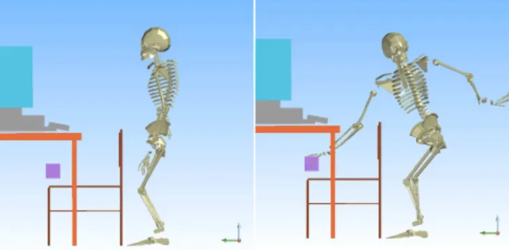
Fig. 1. Reaching for an object in a constrained area
B. Randomized Motion Planning
The other toolkit at our disposal is randomized motion planning. In the past fifteen years, several ways of randomly exploring the configuration space (CS) have been success-fully proposed ([3], [13], [15], [11], [9]). These methods have been shown to be efficient for planning collision-free paths for high dimensional systems.
Their application to humanoid robots, however, is not straightforward, as constraints other than collision avoidance must be taken care of. [12] proposes a whole-body motion planning method that deals with obstacle avoidance and dy-namic balance constraints. It explores a set of pre-computed statically stable postures with a RRT-like algorithm and then filters the configuration space path into a dynamically stable trajectory. [19] deals with global motion planning under task constraints. The method is also an extension of the RRT algorithm, where the sampled configurations are projected on the sub-manifold of CS that solves a task. The limit of this work is that it only considers very specific constraints, basically restrictions on a robot end-effector motion rela-tively to some world fixed frame. This is not sufficient to solve problems such as static stability, which can be seen as positioning an abstract end-effector -the center of mass of the robot- within a given region. A similar drawback is that it can not deal with multiple and prioritized constraints, whereas the corresponding local jacobian methods exist in the literature. More recently, a method similar to ours has been presented and used on manipulator arms in [2].
Finally, the problem we address is related with motion planning for closed kinematics chains. Some random tech-niques have been proposed to solve these problems ([4], [16]). It differs from our work by the fact that the task is solved by random techniques rather than jacobian based optimization.
C. Contribution
The work presented here proposes a new way to use local jacobian based methods within randomized motion planning. The local methods are more generic than the ones in [19], which makes our algorithm usable for solving humanoid whole-body motion planning. It differs from [7] and [8] by the way we treat obstacle avoidance, i.e. not in the optimization loop. The experimental section will show that it is a relevant choice in terms of computation time for complex problems.
Before going further and detailing our method, note that we only address the problem of finding statically stable
paths for humanoid robots. To transform these paths into dynamically stable trajectories, we would need to use an-other optimization stage, as it is presented in [12] and [8] for instance. As this second stage is independent from the first one, we chose not to deal with it here.
D. Paper Outline
Next section recalls the different techniques we use in our algorithm: on one hand a random path planning algorithm, on the other hand a prioritized kinematic constraint solver. Section IV presents the algorithm itself and section V the use examples on different scenarios, as well as comparisons with some existing methods for whole-body motion planning.
III. PRELIMINARIES
A. RRT-Connect
This work considers humanoid whole-body motion plan-ning problems. Because of the stability constraints and of the way the goal is expressed (as a task and not as a final con-figuration to achieve), we can not use classic generic motion planning algorithms. However, we did use an architecture similar to random diffusion methods, and more precisely to what is known in literature as RRT-Connect ([11]). Let us remind briefly the structure of that algorithm.
Algorithm 1 shows the pseudo-code of the RRT algorithm. It takes as input an initial configurationq0and grows a tree T in CS. At each step of diffusion, it samples a random configurationqrand, finds the nearest configuration to qrand in T : qnear, and extends T from qnear in the direction of qrand. The original version of RRT-Connect depends on a step parameter ε. Each step of extension adds as many collision-free nodes to T as possible in direction of qrand, each node being at a distanceε from the previous one. Fig. 2 shows one step of extension of the RRT-Connect algorithm.
qnear
T
ε ε ε
new configurations
qrand
Fig. 2. One step of extension of the RRT-Connect algorithm
Algorithm 1 RRT-Connect(q0) T .Init(q0) fori = 1 to K do qrand← Rand(CS) qnear ← Nearest(qrand, T ) Connect(qnear, qrand) end for
B. Local Path Planning under Task Constraints
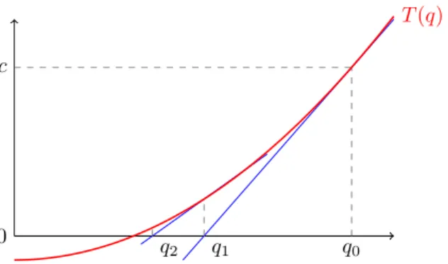
The tasks we consider for the robot can be expressed as a goal value for some functionT of the robot configuration q: T (q) = 0. Assume the current configuration has a value T (q) = c. By computing the jacobian J = ∂T
∂q(q), one can calculate velocities ˙q that tend to achieve the task. ˙q is solution of the linear system:
J ˙q = −λc (1) whereλ is a positive real.
If the robot is redundant enough, i.e. if that linear system is underconstrained, we can solve other lower prioritized tasks at the same time, by keeping ˙q in the affine space solution of eq. (1). Iterating (1) is known as the Newton-Raphson method. Fig. 3 shows a 1-D example of a zero approximation by this algorithm.
The precise implementation of the local planner we use is described in [20]. During global planning, we will consider several types of tasks for various reasons:
• Static stability: the center of mass of the robot should stay at the vertical of the support polygon center; if we are planning a dual support motion, the two feet should remain at the same position and orientation. These tasks should always be achieved.
• Goal achievement: the robot should at some point not only exploreCS but achieve some particular goal task. The ones we will present in the experimental section are reaching a particular point with the hand and open a door ; the hand should then stay on a given arc of a circle.
• Configuration space exploration: as we will explain in more details in the next section, we use configuration space defined tasks to exploreCS.
0 q 0 c q1 q2 T (q)
IV. RANDOMIZED TASK PLANNING FOR A HUMANOID ROBOT
This section describes the global whole-body motion plan-ner. The core of it is a RRT-Connect algorithm. Some tasks have to be achieved for every configuration in the growing tree. This is the case for instance for stability tasks as well as for the position of the hand of the robot during a door opening motion. We will refer to these tasks as constraints. Next paragraph explains how we change the Connect function of the RRT algorithm to comply with these constraints.
A. Task Constrained Extension
Starting from a configuration qnear that respects a set of constraints, we want to go as far as possible in another configuration (qrand) direction, while keeping the constraints verified. To do so, we add a task to the local planner, whose value is the distance, in CS, to a given configuration. It is referred to as Conf igurationT ask in algorithm 2. This task is added with the lowest priority. The configurations we try to reach are successively the ones a classical RRT would have added to the tree. Fig. 4 shows one step of constrained extension. After calling the local planner, we check that the configurations it outputted respect indeed the constraints, that they are collision free, and that the edges linking them together are collision free as well. Algorithm 2 shows pseudo-code for one call to the Constrained-Connect function.
Algorithm 2 Constrained-Connect(T , qnear, qrand) T asks.Initiate(Constraints)
T asks.Add(Conf igurationT ask)
∆q ← ε.(qrand− qnear)/||(qrand− qnear)|| qtarget← qnear+ ∆q
qcurrent← qnear State ← Progressing
whileState = Progressing do
Conf igurationT ask.SetTarget(qtarget)
qnew← LocalPlannerPerformOneStep(T asks, qcurrent) ifqnew6= qcurrent
and CollisionCheck(qnew) = OK
and CollisionCheckEdge(qcurrent, qnew) = OK and ConstraintsCheck(qnew) = OK then
T .AddNode(qnew)
T .AddEdge(qcurrent, qnew) qcurrent← qnew
ifqtarget6= qrand then qtarget ← qtarget+ ∆q else State ← Reached end if else State ← Trapped end if end while Constrained manifold qnear qrand new configurations
Fig. 4. One step of constrained extension
B. Goal Configuration Generation
One main difference between the problems we consider and classic motion planning is that the goal configuration is not defined explicitly. Instead, the input of the planner is a given task in the workspace. The output of the planner should therefore be a statically stable, collision-free path between the initial configuration and a configuration that solves the goal task. There are many ways to adapt motion planners to do so. One could be to grow a tree in CS and try from time to time to apply the goal task to a newly generated configuration, hoping that the local planner will return a collision-free path that solves the problem. This option is available in our planner, simply by changing the task to solve in the Constrained-Connect function. However, we found it more efficient to generate random goal configurations, using the local planner, and then express the problem as a classic motion planning one, with one initial configuration and several goal configurations. The reason is that once we have defined explicit goal configurations, we can root random trees at those configurations. The idea of growing a tree rooted at the final configuration was first proposed in [11]. Generating several goals for manipulation planning was proposed in [5]. Another way of looking at that problem is the formalism of task maps [6].
The way we generate a goal configuration is the following: 1) Shoot a random configuration in CS with uniform
distribution.
2) Call the local planner on this configuration, with the static stability constraints and the goal task.
3) Check that all of those tasks are achieved. 4) Check for collisions.
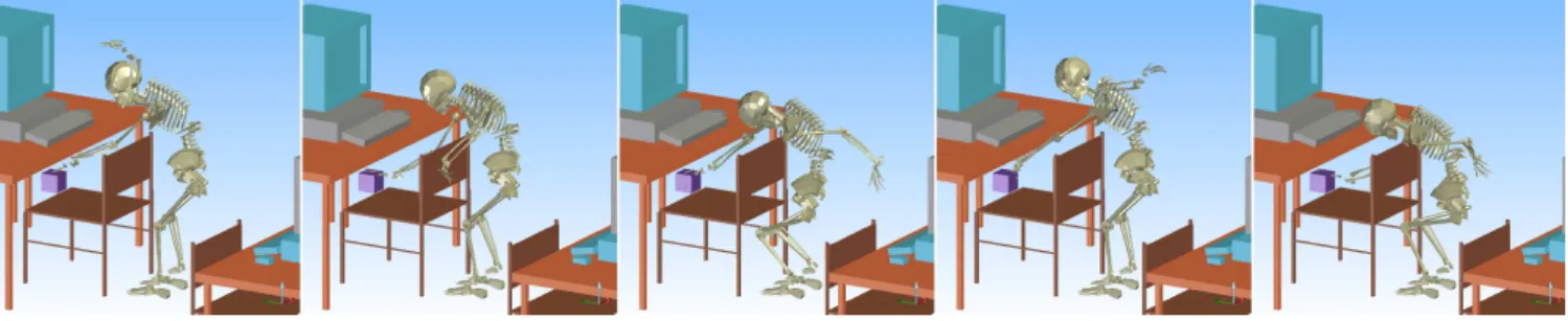
Fig. 5 shows different random goal configurations respect-ing stability and goal constraints.
Probabilistic completeness: Guaranteeing probabilistic completeness is not as straight forward for task planning as for classical configuration to configuration planning. The reason is that we do not know explicitly the shape of the solution manifold. Some solutions may not be in the same connected component as the initial configuration while some other are. If we choose to first shoot random goal configura-tions, we must ensure that any neighbourhood of the solution manifold has a positive probability of being reached. This is the case with our way of shooting the goals configurations. Reciprocally, if a collision-free, statically stable solution path exists, we have a positive probability of shooting a goal configuration in the neighbourhood of that path’s final
Fig. 5. Random goal configurations solving the reaching task. All the configurations are stable and collision-free.
Fig. 6. Different steps of a posture optimization. All the configurations respect the stability and goal constraints, and the configurations are more and more natural.
configuration, then a positive probability of growing a branch of the tree in a neighbourhood of the path. This latter claim comes from the fact that the local planner can extend the tree in any direction along the sub manifold of the configuration space corresponding to statically stable configurations. This ensures our algorithm’s probabilistic completeness.
C. Posture Optimization
As in classic motion planning, once we have found a random solution path, it is important to optimize it. The criteria to optimize depend on the system. In humanoid robotics, the motion should look “realistic” or “natural”, for any good definition of these concepts. As the goal configuration we have reached as the end of the solution path was generated randomly, we need to optimize it as well. Note that we only optimize it after having found a solution path because we do not want to optimize useless goal configurations.
To optimize the posture, we use a random gradient descent algorithm, starting from the configuration to optimize. The local planner ensures that all the constraints (stability and goal task) are achieved and is repetitively called to generate collision-free random displacements that minimizes a certain “natural” cost function. In the presented examples, that function was theCS distance to a reference posture. The new solution path is the concatenation of the previous solution and the path resulting from the posture optimization.
Fig. 6 shows the different steps of a goal posture opti-mization.
D. General Architecture
Now that we have all the tools at our disposal, the architecture of the planner can be explained.
1) First we generate several goal configurations.
2) We search for a path between the initial configura-tion and one of the goal configuraconfigura-tions with a RRT algorithm. We can either grow a single tree rooted at the initial configuration or several other trees rooted at each of the goal configurations.
3) If a path is found, we optimize the reached goal posture.
4) We optimize the concatenation of the solution path and the posture optimization one with classic random motion planning path optimization methods.
During the RRT search and the final path optimization, we use the task constrained extension detailed earlier.
V. EXAMPLES
This section presents experimental results of our whole-body motion planner on simulations on the robot HRP2. We compared it thoroughly with the local collision avoidance method presented in [7] on two different examples of hand reaching motion. One is a dual support motion, where the humanoid robot has to reach an object under a table, and the other one is a more complicated single support motion, where the robot should reach a point inside a large torus shaped obstacle. These comparison were made to evaluate the relevancy of avoiding obstacles at a global scale rather than inside the optimization loop.
The implementation of our algorithm uses KineoWorksTM([14]) implementation of random diffusion algorithms and collision checking. All the simulations were performed on a 2.13 GHz Intel Core 2 Duo PC with 2 GB RAM. Note that the figures taken from [7] and [8] were obtained on a similar PC, so time comparisons are relevant here. For each problem, we ran the planner ten times: this includes goal configuration generation, path planning,
TABLE I
COMPUTATIONAL TIME(MS)FOR THE PRESENTED SCENARIOS.
Goal Generation Path Planning Posture Optimization Path Optimization Local Planner Collision Detector Table 281 4,017 16,181 5,096 1.25 % 86 % Torus 1,689 27,965 40,479 23,851 9.19 % 84 %
Fig. 8. Solution path for “Torus” scenario.
Fig. 7. Solution path for “Table” scenario.
posture optimization and whole-body path optimization. We indicated the cost of each of these computations, as well as the relative costs of the collision detector and the local task solver. Those last costs are expressed as percentages of the total computational time. They do not add up to 100 %. The rest of the time is spent in roadmap and environment management.
A. Dual Support ”Table” Scenario
Fig. 7 shows the solution path for a problem of reaching an object under a table. A similar experiment was presented in [7]. The local method presented in [7] computes one step of optimization in about 100 ms for this problem; it can therefore run at half the speed required for real time when selecting a time step of 50 ms. The trajectory lasts 14 s so the planning time is about 28 s.
Table I shows the time taken by our planner. The average total time, including both planning and optimization, is 25.6 s. Note that most of the time is spent with posture and path optimization. Problem solving itself (goal generation and path planning) only lasts 4.3 s. However, optimization is mandatory since we are using random path planning method. It is indeed the total time that should be compared to the 28 s found in [7].
B. Single Support “Torus” Scenario
Fig. 8 shows the solution path for a more complex prob-lem. The robot is on one foot and has to reach a point inside a large torus shaped obstacle. Table I shows the time taken by our planner. This problem was presented in [8]. It is a very difficult problem for a local method dealing with obstacle avoidance because of the complexity and proximity of the obstacles. When computing this motion with the precise models of both the robot and the torus, the local method for obstacle avoidance takes 1.47 s per step. The reason is that there are 3460 constraints induced by the collision avoidance. [8] presents simplified models of the robot and the torus, which leads to a computational time of 50 ms per step (375 constraints). The generated trajectory lasts 77 s (before dynamic optimization). The planning time is then about 77 s for the simplified models and 1540 s for the precise models. Table I shows the time taken by our planner. The average total time is 94.0 s and the problem solving itself is 29.7 s. Once again, most of the time is spent optimizing the results. The local task solver is comparatively more costly for this problem, one explanation might be that the stability constraint is more difficult to compute for single foot support.
C. When to Deal with Obstacle Avoidance
It is difficult to compare our planner with a local collision avoidance method because they are not intended for the same use. The local collision avoidance method can be used as a controller, while our work is really about offline planning. However, what we can say is that the cost of collision avoidance constraints make the local method unusable on complex examples. On the other hand, our probabilistic planner can be used to compute -in a reasonable time- a statically stable, collision-free path that could be executed afterwords by a controller. Note that it does not mean that local collision avoidance methods are hopeless, but for now, they can only be used on simplified or dedicated models. For instance, if the robot and the obstacles were modeled by spheres or smooth curves (with analytical formulas for distance computation) rather than triangles, the number of
constraints induced by collision avoidance would decrease and the computational time would be drastically reduced.
VI. CONCLUSION
In this paper, we have presented a novel whole-body plan-ning method for humanoid robots. It uses a local task solver to generate valid configurations within a random diffusion algorithm framework. Its advantages are the generality of the local task solver, which makes the planner usable for a large variety of problems,including for instance stability constraints for a humanoid robot, and the efficiency of random diffusion algorithms for high dimensional problems, evaluated through computation time comparison. We have compared our approach with a local method for collision avoidance. The results show that for complex scenarios, the planning time can be more than an order of magnitude lower with random planning than with local obstacle avoidance.
VII. ACKNOWLEDGMENTS
This work was supported by a LAAS-CNRS and Toyota Motor Europe NV/SA cooperation contract.
REFERENCES
[1] P. Baerlocher and R. Boulic. Task-priority formulations for the kinematic control of highly redundant articulated structures. In 1998
IEEE/RSJ International Conference on Intelligent Robots and Systems, 1998. Proceedings., volume 1, 1998.
[2] Dmitry Berenson, Siddhartha S. Srinivasa, Dave Ferguson, and James J. Kuffner. Manipulation planning on constraint manifolds. In Robotics and Automation, 2009. ICRA ’09. IEEE International
Conference on, pages 625–632, May 2009.
[3] H. Choset, KM Lynch, S. Hutchinson, GA Kantor, W. Burgard, LE Kavraki, and S. Thrun. Principles of Robot Motion: theory, algorithms, and implementation. MIT Press, 2005.
[4] J. Cortes, T. Simeon, and JP Laumond. A random loop generator for planning the motions of closed kinematic chains using PRM methods. Robotics and Automation, 2002. Proceedings. ICRA’02. IEEE International Conference on, 2, 2002.
[5] R. Diankov, N. Ratliff, D. Ferguson, S. Srinivasa, and J. Kuffner. Bispace planning: Concurrent multi-space exploration. Proceedings
of Robotics: Science and Systems IV, 2008.
[6] M. Gienger, M. Toussaint, and C. Goerick. Task maps in humanoid robot manipulation. In Intelligent Robots and Systems, 2008. IROS
2008. IEEE/RSJ International Conference on, pages 2758–2764, Sept. 2008.
[7] F. Kanehiro, F. Lamiraux, O. Kanoun, E. Yoshida, and JP Laumond. A Local Collision Avoidance Method for Non-strictly Convex Polyhedra. In 2008 Robotics: Science and Systems Conference, 2008.
[8] F. Kanehiro, W. Suleiman, F. Lamiraux, E. Yoshida, and J.P. Laumond. Integrating Dynamics into Motion Planning for Humanoid Robots. In
IEEE/RSJ International Conference on Intelligent Robots and Systems, 2008. IROS 2008, pages 660–667, 2008.
[9] LE Kavraki, P. Svestka, J.C. Latombe, and MH Overmars. Proba-bilistic roadmaps for path planning in high-dimensional configuration spaces. Robotics and Automation, IEEE Transactions on, 12(4):566– 580, 1996.
[10] O. Khatib, L. Sentis, J. Park, and J. Warren. Whole body dynamic behavior and control of human-like robots. International Journal of
Humanoid Robotics, 1(1):29–43, 2004.
[11] J. Kuffner and S. LaValle. RRT-connect: An efficient approach to single-query path planning. In Proc. IEEE Int’l Conf. on Robotics
and Automation (ICRA’2000), San Francisco, CA, April 2000. [12] J.J. Kuffner, S. Kagami, K. Nishiwaki, M. Inaba, and H. Inoue.
Dynamically-stable motion planning for humanoid robots. Au-tonomous Robots, 12(1):105–118, 2002.
[13] J.C. Latombe. Robot Motion Planning. Kluwer Academic Publishers, 1991.
[14] J.P. Laumond. Kineo CAM: a success story of motion planning algorithms. Robotics & Automation Magazine, IEEE, 13(2):90–93, 2006.
[15] S. M. LaValle. Planning Algorithms. Cambridge University Press, Cambridge, U.K., 2006. Available at http://planning.cs.uiuc.edu/. [16] SM LaValle, JH Yakey, and LE Kavraki. A probabilistic roadmap
approach for systems with closed kinematicchains. In 1999 IEEE
International Conference on Robotics and Automation, 1999. Proceed-ings, volume 3, 1999.
[17] Y. Nakamura and H. Hanafusa. Inverse kinematic solutions with singu-larity robustness for robot manipulator control. ASME, Transactions,
Journal of Dynamic Systems, Measurement, and Control, 108:163– 171, 1986.
[18] B. Siciliano and J.J.E. Slotine. A general framework for managing multiple tasks in highly redundant robotic systems. In Advanced
Robotics, 1991.’Robots in Unstructured Environments’, 91 ICAR., Fifth International Conference on, pages 1211–1216, 1991.
[19] M. Stilman. Task constrained motion planning in robot joint space. In
Proc. of the IEEE/RSJ Intl. Conf. on Intelligent Robots and Systems, pages 3074–3081. Citeseer, 2007.
[20] E. Yoshida, O. Kanoun, C. Esteves, and J.P. Laumond. Task-driven support polygon reshaping for humanoids. In Humanoid Robots, 2006