HAL Id: hal-01591373
https://hal.archives-ouvertes.fr/hal-01591373
Submitted on 21 Sep 2017
HAL is a multi-disciplinary open access
archive for the deposit and dissemination of
sci-entific research documents, whether they are
pub-lished or not. The documents may come from
teaching and research institutions in France or
abroad, or from public or private research centers.
L’archive ouverte pluridisciplinaire HAL, est
destinée au dépôt et à la diffusion de documents
scientifiques de niveau recherche, publiés ou non,
émanant des établissements d’enseignement et de
recherche français ou étrangers, des laboratoires
publics ou privés.
Using a Memory of Motion to Efficiently Warm-Start a
Nonlinear Predictive Controller
Nicolas Mansard, Andrea del Prete, Mathieu Geisert, Steve Tonneau, Olivier
Stasse
To cite this version:
Nicolas Mansard, Andrea del Prete, Mathieu Geisert, Steve Tonneau, Olivier Stasse. Using a Memory
of Motion to Efficiently Warm-Start a Nonlinear Predictive Controller. IEEE International Conference
on Robotics and Automation (ICRA 2018), May 2018, Brisbane, Australia. 9p. �hal-01591373�
Using a Memory of Motion to Efficiently Warm-Start
a Nonlinear Predictive Controller
N. Mansard
1, A. Del Prete
1, M. Geisert
1, S. Tonneau
1, O. Stasse
1Abstract— Predictive control is an efficient model-based methodology to control complex dynamical systems. In general, it boils down to the resolution at each control cycle of a large nonlinear optimization problem. A critical issue is then to provide a good guess to initialize the nonlinear solver so as to speed up convergence. This is particularly important when disturbances or changes in the environment prevent the use of the trajectory computed at the previous control cycle as initial guess. In this paper, we introduce an original and very efficient solution to automatically build this initial guess. We propose to rely on off-line computation to build an approximation of the optimal trajectories, that can be used on-line to initialize the predictive controller. To that end, we combined the use of sampling-based planning, policy learning with generic representations (such as neural networks), and direct optimal control. We first propose an algorithm to simultaneously build a kinodynamic probabilistic roadmap (PRM) and approximate value function and control policy. This algorithm quickly converges toward an approximation of the optimal state-control trajectories (along with an optimal PRM). Then, we propose two methods to store the optimal trajectories and use them to initialize the predictive controller. We experimentally show that directly storing the state-control trajectories leads the predictive controller to quickly converges (2 to 5 iterations) toward the (global) optimal solution. The results are validated in simulation with an unmanned aerial vehicle (UAV) and other dynamical systems.
I. INTRODUCTION
This paper focuses on the control of complex dynamical systems such as UAVs and legged robots. Classical control approaches are hardly applicable to these systems, which represent thus an open problem for the robotics community. Different techniques exist to control complex dynamical systems, most of which can be labeled either as model based, or as model free.
Model-based approaches, such as Model Predictive Con-trol (MPC), exploit a model of the system to find the conCon-trol inputs that drive it towards a desired state. Despite their remarkable capabilities and their wide use in robotics, they are severely limited by the associated computation time, which makes their application to large systems extremely challenging. Moreover, model-based techniques need to face the problem of modeling errors, which negatively affect their performance on real hardware.
At the other end of the spectrum we find model-free approaches, such as reinforcement learning [1]. These approaches can learn—either by trial and error or by demonstration—how to control a system to achieve a speci-fied task. Model-free techniques shine exactly where model-based techniques struggle, that is in their computation time
1
CNRS - LAAS, Toulouse, France,[email protected]
and in their adaptation capabilities. However, the off-line learning phase may require unacceptable training times for large systems. Moreover, these techniques need an exhaustive exploration of the state space in order to perform reliably, which in general cannot be ensured.
Given the complementary nature of model-based and model-free approaches, many ways to combine them have been proposed. We can observe two main families of ap-proaches:
1) Using model-based techniques to speed up the training of model-free techniques.
2) Learning models/functions to improve the performance of model-based techniques.
In the first family we can find works from both robotics and computer graphics, where local trajectory optimization has been used to guide the search of a desired control policy [2], [3], [4]. This allows to speed up the training phase (of neural networks in these specific cases) and thus to explore a larger part of the state space. However, this does not completely solve the issue of reliability of the resulting controller, and it needs an extremely accurate learning to avoid unstable control policies.
In the second family we can find different techniques, most of which boil down to learning a certain function off-line, and then using this function on-line inside an MPC. The learned function can be the Value function [5], the system dynamics model [6], or the cost function [7]. The main goal is always to speed-up the MPC computation time and/or to improve the quality of the computed solution. Earlier versions of the same idea consisted in storing a library of optimal trajectories computed off-line, and then use nearest-neighbor to recover the control trajectories to use on-line [8]. The same concept has been applied also to sampling-based planning, where the Value function has been learned to improve the quality of an RRT [9]. Similarly, trajectory optimization has been used to alleviate the curse of dimensionality of dynamic programming [10].
This work combines the two above-mentioned families: we first use model-based techniques to learn off-line a control policy, which we then use on-line to warm-start an MPC. With respect to previous work we present several peculiarities:
• In the off-line training phase we combine a local trajectory optimization with a sampling-based motion planner (PRM) to compute better sample trajectories. This allows us to learn a better control policy with respect to using only a local trajectory optimization.
• Rather than generating the sample trajectories and learn-ing the control policy in sequence, we do it in a cyclic way. After learning the control policy, we use it to improve the PRM, thus leading to an even better quality of the sample trajectories.
• We use the learned policy to initialize the MPC, rather than to modify the problem definition. This makes the system more reliable because the learned function does not affect the problem we are solving, but only the starting point of the search.
• We show that rather than learning the control policy we can learn the future state and control trajectories. De-spite the higher dimensionality of the learning problem, this approach gave much better results in our tests, and it avoids the need of performing a roll out to retrieve the trajectories from the policy.
II. BACKGROUND:OPTIMAL CONTROL AND KINODYNAMIC PLANNING
We consider here the problem of finding the (global) minimum of an optimal control problem, i.e computing optimal control and state trajectories of an arbitrary dynamic system in its environment.
A. Dynamic model
We denote by x∈ X the state of the system (typically a vector of dimension nx, possibly representing an element of a Lie group) and by u∈ U its control vector (living in a vector space of dimension nu). We denote byΩ a parametrization of the environment where the system evolves (e.g. obstacle location, external disturbances, time-dependent uncontrolled dynamic effects).
We consider an autonomous dynamics (time independent): ˙x = f (x, u, Ω) (1) We denote by X : t → X and U : t → U the trajectories in state and control spaces. X and U are constrained together to respect (1).
B. Optimal control
Among all admissible trajectories X, U , we are interested in the pairs that minimize a cost functional L(X, U ). The functional is typically composed of an integral cost term and a terminal cost term, that encodes the task to be achieved by the system. The optimal trajectory starting from an arbitrary state x0∈ X is the solution of the following optimal control problem: minimize X∈X ,U ∈U , T >0 L(X, U ) subject to ˙x(t) = f (x(t), u(t), Ω), ∀t ∈ [0, T ] x(0) = x0 (2)
where the decision variable T is the duration of the preview interval. We suppose that (2) has a unique minimum (no redundancy). Moreover, we suppose that L is sufficiently constraining to bring the trajectory to end at—or close to—a desired state. More specifically, we do not consider here the
typical terminal constraint x(t) = x∗
, while some terms in L should play a similar role.
Additional constraints can also be considered (typical state limits, obstacle avoidance, etc are supposed to be encoded inX and U ).
C. Value function and optimal policy
For any initial state x∈ X and environment Ω, we denote by V(x, Ω) the Value function, i.e. the optimal cost of (2) for x0 = x. We denote by π(x, Ω) the policy function, i.e. the optimal control to apply to get the optimal cost. Finally, we denote by X∗(x, Ω), U∗
(x, Ω) the optimal state and control trajectories.
We are interested in robotic systems where it is typically not possible to obtain an analytical expression of V , π, X∗ and U∗. We are then doomed to approximate these functions by numerical methods.
Dynamic programming tends to globally solve the prob-lem, by integrating over the whole state space. It is thus limited by the curse of dimensionality. On the other hand, direct trajectory optimization only considers one trajectory at a time. Any discretization (i.e piecewise constant, poly-nomial, etc) of the control and/or state trajectories is chosen by the user. Problem (2) is then converted into a standard optimization problem (i.e. with a finite number of decision variables), which is solved by an iterative descent algorithm (typically a Gauss-Newton sequential quadratic program). In the design of the numerical algorithm, care has to been taken to the sparsity and the numerical conditioning of the problem. Well-known algorithms are Differential Dynamic Programming (DDP) [11], its Gauss-Newton approximation (iterative LQR) [12], and multiple-shooting [13]. Off-the-shelf implementations of any of these algorithms are easily available.
While the original optimal-control problem is character-ized by global optimality principles (due to Pontryagin and Bellman), their static approximation is most of the time a non-convex optimization problem, only characterized by local optimality principles. The direct consequence is that the corresponding algorithms are likely to end in poor local optima, sometimes not even able to converge to any relevant solution at all.
To avoid this, it is necessary to give an initial guess that the optimizer can use to initiate its search. This is true in particular when the initial state x0is far from the goal region, and when it is important that the solver converges quickly. When no heuristic initial guess is available (i.e. in the general case), we can compute one of these complex trajectories relying on sampling-based methods.
D. Kinodynamic planning
Kinodynamic planning is a class of problem considering generic dynamical systems that cannot follow static trajecto-ries. Kinodynamic planners sample the state spaces and try to connect the sampled states with trajectories respecting (1). Nodes (i.e. states) are connected by a local controller, which we call a steering method: it is a function that maps any pair
of states to a connecting trajectory. By definition, we suppose that the steering method is local, i.e. is only able to connect two states if they are “close enough”. The major stake of kinodynamic planning algorithms is to properly define this “close enough”. Given two states x1, x2, we need a metric function to define how close these points are, i.e. how likely the steering method will be able to connect them. This is where kinodynamic planning is correlated with optimal control.
Suppose that the steering method can be modeled as an op-timal control problem (with initial and terminal constraints).
minimize X∈X ,U ∈U , T >0 L(X, U ) subject to ˙x(t) = f (x(t), u(t), Ω), ∀t ∈ [0, T ] x(0) = x0, x(T ) = x1 (3)
The value, policy and optimal trajectory functions now depend on both the initial and the final state (e.g. V , V (x0, x1,Ω)). Then a proper metric in the state space is given by the value function.
III. ITERATIVE ROADMAP EXTENSION AND POLICY APPROXIMATION
A. Steering method, metrics and visibility
We define the visibility region as the state space region around a state x0 that can be connected to x0 with the steering method. We also define the visibility range as the scalar characterizing the size of the minimal visibility region. Ideally, a kinodynamic planner should sample new states on the border of the visibility region and only try to connect them to previously-sampled states within the visibility range. In practice, the visibility border cannot be directly sampled. The state space is rather uniformally sampled, while connec-tions are tried only toward the closest points (in the sense of the metrics).
Since neither the visibility range nor the exact value function can be computed in the general case, the efficiency of the planner then depends on the visibility range of the steering method, and on the accuracy of the value-function approximation.
B. Algorithm hypotheses and principles
We consider here that a local trajectory optimizer is available to solve (3). The main hypothesis is that this solver outputs the global optimum when the initial and terminal points are close enough1. Under this hypothesis, any regular metrics makes the classical sampling-based kinodynamic planner probabilistically complete (i.e. able to find a path toward any desired state).
Our objective is to use the local trajectory optimizer to compute the control law of the robot in real time. For that, the visibility radius must be enlarged so that any admissible starting state is visible from the goal. We propose to iteratively build i) a kinodynamic PRM whose edges are
1We suppose that, ∀x
0 ∈ X, ∃ǫ > 0, such that any x1 in theǫ-ball
aroundx0can be connected by a globally-optimum trajectory.
locally optimal with respect to (3) and ii) an approximation of the functions V, π, X∗ and U∗ (see Section III-C) based on the trajectories stored in the PRM (see Section III-D).
The function approximators are then used to guide the steering method (see Section III-E), hence enlarging its visibility radius. Consequently, each new iteration improves the cost associated to the PRM edges, hence the quality of the approximators. The main difficulty is to make sure that the PRM edges and the function approximators are consistent (see Section III-F). At convergence of the algorithm, any pair of nodes of the PRM can be directly connected using the steering method guided by the approximators.
C. Value and policy approximator
We can approximate the value and policy functions by any generic parametric model. In our experiments, we used 2-layer neural networks with ELU and hyperbolic functions, although any other parametric model is likely to work similarly.The approximator is then a function of the states and the parameters:
V(x0, x1,Ω) ≈ ˆV(x0, x1,Ω|αV) π(x0, x1,Ω) ≈ ˆπ(x0, x1,Ω|απ) Similar approximators can be built for X∗
and U∗ .
It is important that the approximators and their gradients with respect the parameters α can be efficiently evaluated. D. Improving the approximation from the PRM
The edges of the PRM are locally-optimal trajectories. Any subtrajectory of the edges corresponds to an example of evaluation of the functions V, π, X∗
, U∗ .
These evaluations are possibly noisy, and possibly subop-timal. We train the approximators to minimize the residual mean squares (RMS) error:
min α
X subtraj ˜X
|| ˆV(˜x0,x1,˜ Ω|α) − ˜V||2
where x˜0,x˜1 are the boundaries of each subtrajectories ˜X and ˜V is its cost.
In practice, we limit the minimal duration of the subtrajec-tories to 20ms. A PRM containing 100s of trajecsubtrajec-tories will then corresponds to around 10.000 subtrajectories. We solve this problem with stochastic gradient descent, using mini-batches (128 items) of subtrajectories. Ten epochs (i.e. 1000 gradient descents with mini-batches of size 128) are suffi-cient to reach a stable RMS error. Even after convergence, we do not expect the RMS error to be close to zero due to the outliers in the dataset.
E. Expanding the graph using the approximators
The approximators are used twice in the PRM expansion. First, the Value approximation is used as a metric to find the nearest neighbors. Second, we initialize the steering method with an approximation of the optimal trajectory.
Using a better approximation of the Value function results in less failures of the local steering method when trying to connect new sampled nodes to the existing graph.
More interestingly, using a better initialization of the steering method increases its visibility range. This allows us to connect nodes that are further away from each other, speeding up the PRM expansion.
F. PRM and approximation consistency
In a PRM, we are generally interested by the connectivity (a path that connects any pair of nodes should exist). In our case, we are also interested in the consistency of the edge trajectories, i.e. two trajectories joining a same goal should not intersect. As the PRM edges are used as a training dataset for improving the approximators, it is important that similar inputs of the dataset corresponds to similar outputs in the region where the function are smooth.
Consistency is clearly obtained at the global optimum of (3). However, without the true Value and policy functions, asserting this property is difficult [10]. We rather assert the consistency by comparing the edges of the PRM with the trajectories stored in the approximators. For each edge of the PRM, we compute the approximated trajectory connecting the associated states.
If the trajectories are different, the stored edge might have a lower cost, a similar cost or a higher cost. A lower PRM cost corresponds to the approximator not having properly stored the corresponding edge yet: we do nothing. A higher PRM cost corresponds to a suboptimal edge: we then recompute the edge trajectory using the steering method initialized with the approximated trajectory.
When the costs are similar, we have to investigate more and compare the trajectory shape using any trajectory metric (for example, integral of the squared distance in the state space). If the distance is significant, it means that several trajectories with similar cost exists for the corresponding state. We then enforce the PRM consistency by replacing the PRM edge with the approximation (refined with the steering method).
G. IREPA algorithm
The previous developments lead to the Iterative Roadmap Expansion and Policy Approximation algorithm (IREPA). The goal of IREPA is to compute a fully connected PRM (i.e. every pair of nodes must be directly connected), together with the corresponding approximators. A consequence of this output is that the resulting steering method (guided by the approximators) can directly connect any pair of nodes in the graph. The algorithm is summarized in pseudo-code in Alg. 1.
We initialize the PRM graph with a given number of nodes and no edge (line #1). At each iteration, we add a given number of nodes in the graph and use the steering method to try to connect the nearest neighbors in the PRM (line #3). At the first iteration, we use the Cartesian metric and no initialization of the steering method. In the following iterations, we use the Value approximation as distance metric and the trajectory approximation to initialize the steering method.
Algorithm 1 Iterative Roadmap Expansion and Policy Ap-proximation (IREPA)
1: Initialize PRM with a given number of state samples
2: repeat
3: Expand PRM
4: stop← True if PRM is fully connected else False
5: Optimize approximator RMS
6: for every edge EP RM in the graph do
7: (x0,x1) ← getStartAndEndNodes(EP RM) 8: Enew ← approximator(x0, x1) 9: if Enew≤ EP RM then 10: Replace EP RM by Enew 11: stop← False 12: end if 13: end for 14: until stop
Once the PRM has been expanded, we update the approx-imators to minimize the RMS with respect to the trajectories stored in the PRM (line #5). Then, we check the consistency of the PRM edges by comparing them to the trajectories stored in the approximation (line #8-9).
The algorithm iterates until every pair of nodes is con-nected and no progress is achieved optimizing the PRM edges (line #4, #11 and #14).
The algorithm is probabilistically complete (as any kino-dynamic PRM): as time increases, the probability that any connected component of the state space will be explored converges toward 1. When bounding the number of nodes, we can also guarantee that the algorithm will stop either with all nodes connected in pairs, or with a subpart of the connections, and with the steering method able to generate all the computed connections directly.
In practice, we have observed that the algorithm converges to the global optimum of (3), i.e. Value and policy functions respect the Hamilton-Jacobi-Bellman equation, and the edges are globally-optimal trajectories. Probabilistic completeness is achieved in the worst case in adding an infinite number of node. In practice, we typically bound the number of nodes in the PRM. A watchdog has then to be added to assert that the algorithm is not trapped in a local minimum where the RMS converges while the steering method fails to discover new edges (again, adding new nodes would untrap the algorithm).
IV. PREDICTIVE CONTROL USING APPROXIMATELY-OPTIMAL INITIAL GUESS
We now suppose that the approximator functions have been properly trained off-line. We detail how these approxi-mations can be used to properly initialize the direct optimal control solver. The main objective is to use this initialization on-line during the control of the robot. However, the same initialization is used for the steering method during the PRM expansion.
A. Importance of the warm-start
As predictive control often boils down to the resolution of a nonlinear non-convex optimization problem, the impor-tance of guiding the search is well recognized. In particular, it should be recalled that no iterative descent algorithm can be guaranteed to converge to a good optimum (either the global optimum, or even a good local optimum) if initialized outside of the basin of attraction of the optimum. As most solvers used for optimal control are Newton or Gauss-Newton solvers, the initialization should even occur in a region around the optimum where the cost function is convex. In general, it is not possible to guarantee this condition.
Predictive control, also called receding-horizon control, often starts the search with the trajectory optimized at the previous control cycle, shifted backward following the reced-ing horizon. The optimization cycle then just needs to adjust the start of the trajectory to the new sensor measurements, and to explore a fraction of time at the end of the horizon.
However, this initialization may not be sufficient when the robot faces large disturbances, or when the environment changes suddently, or when the configuration at the end of the horizon is particularly unstable. These situations are typical of many robots, in particular UAVs (often facing large disturbances with unstable horizon) and legged robots (drastic changes at each new foot contact).
B. Storing the initial guess
Several ways to store the initial guess exist. A common choice is to store an approximation of the policy function. A trajectory from a given state x0 is then obtained by rolling out the policy and integrating it using the dynamic model. This method produces both a state and a control trajectory.
Alternatively, we can store an approximation of these two functionals directly. The trajectories can be represented by any discretization (e.g. passing points, splines or Bezier coefficients, etc). We then approximate the function that maps every point of the state space to the discretization parameters. In this case, it is difficult to enforce the dynamic consistency of the two resulting approximations. However, this would be quickly corrected by the trajectory optimizer. Approximating the policy is more compact, as the trajec-tory discretization lives in a space larger than the control space. In a sense, the policy approximation exploits the recursivity of the control spaces, that the trajectory approx-imation fails to capture. Moreover, the trajectories obtained by roll-out respect the dynamic model. On the other hand, the roll-out is subject to the (typical) instability of the dynamic model. A small error in the policy approximation is likely to result in a large error in the generated trajectories, as the error is amplified by the dynamics. Moreover, the roll-out might be more expensive to compute.
An alternative would be to approximate the function that maps the current state to the next key state, along with a parametrization of the control trajectory needed to reach it. This solution would avoid the instability of the dynamic roll-out while capturing the recursivity of the control. While approximating the key states seems an appealing solution,
we were not able to obtained satisfying results with this approach. We are not yet able to explain why.
C. Perspectives about alternative guiding techniques In this work we decided to guide the optimal control solver by initializing the search (i.e. warm start). However, other guiding techniques might be considered. We could add a guiding term to the cost function, whose importance would be decreased as the optimizer iterates. Such a homotopy optimization is used e.g. in interior point solvers (the log barrier weight is decreased at each iteration) or in the contact-invariant optimization [14]. An evident candidate here would be to add a term based on the Value function [15], for which we have a good approximation.
Another type of warm-start can be obtained by initializing the descent direction, in particular if the BFGS approxima-tion is used by the solver. Storing some subgradients was exploited in computer vision [16], and might also be used here to fasten the first iteration of the search.
V. RESULTS
In this section, we report the results obtained with a planar UAV with two propellers. Trajectories obtained with other dynamic systems are shown in the companion video.
The system has 3 degrees of freedom and 2 control inputs. The small dimension allows us to more easily plot the behavior of the algorithms and the resulting trajectories of the system. We start by reporting the technical details of our tests. Then we present the main results divided in off-line phase (IREPA algorithm) first, and on-off-line phase (warm start) last.
A. Setup
1) System dynamics and cost: The UAV is modeled by a state of dimension 6: two translations x, z, one rotation θ, and the corresponding velocities ˙x, ˙z, ˙θ. The control inputs are the forces f1, f2 applied by the propellers, which must be positive and bounded. The dynamics is:
¨ x= −1 m(f1+ f2)sinθ (4) ¨ y = 1 m(f1+ f2)cosθ − g (5) ¨ θ= l I(f1− f2) (6) where m and I are mass and inertia of the UAV, g is gravity and l is the lever arm of the propeller. We set m= 2.5kg, I = 1.2kg m2
, l = 0.5m, following the dimension of the AscTec Falcon. The propellers are limited to25N , without continuity constraints.
We consider minimum-time trajectory, i.e. the cost func-tion is the trajectory durafunc-tion. Similar results are obtained with minimum-norm running cost.
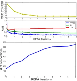
Fig. 1. Evolution of the PRM and the approximators during the IREPA iterations. Top: decrease of the PRM mean edge cost (on a constant subset of 140 edges) and approximator RMS error. Bottom: number of connections between 30 reference nodes.
2) Approximators: We used a neural network to imple-ment the approximator function (Value, policy, trajectories). All networks are implemented with 2 hidden layers with ELU activation function. The output layer of the Value approximator is also activated by ELU, while policy and trajectories output layer are hyperbolic tangent (scaled within range limits).
Trajectories are optimized with the multiple shooting solver ACADO [13], an open-source library that can be used to easily solve various optimal-control problems. Inside ACADO, the control trajectories are represented by piece-wise constant functions (typically 20 intervals), while the state trajectories are obtained from a RK45 integrator.
3) Computational setup: The optimal control solver and neural-network stochastic gradient descent [17] are imple-mented in C++. The rest of the application (planner, IREPA algorithm, etc) is implemented in Python. The tests were run on a single process on a Intel Xeon E5-2620 (2.1GHz). The algorithm would be easy to parallelize: most of the CPU time is consumed by the steering method, which can be run independently on several cores.
B. Off-line phase
We first empirically validate the convergence of IREPA and its efficiency compared to a kinodynamic PRM.
1) IREPA convergence: To better visualize the IREPA converge, we first work with a fixed number of nodes in the PRM (30). Fig. 1 shows several quantities during IREPA convergence. The mean cost on a fixed number of edges (the ones computed in the first iteration) decreases, while better local optimum are computed for the edges thanks to the improved approximators. Reciprocally, we plot the RMS along with the stochastic gradient descent: the RMS error converges to a local minimum at each IREPA iteration. Then, when new and better edges are computed at the next IREPA
Fig. 2. Comparison of the progress of IREPA versus PRM algorithms. Top: IREPA requires less evaluation of its (improved) steering method to establish more connections between distant nodes. Bottom: the connections computed by IREPA have also lower cost.
Fig. 3. Typical examples of the trajectories stored in the PRM (left), in the approximators (middle) and computed by the steering method (right). The trajectories computed in the early IREPA iterations are in light gray, while dark grey is used for the trajectory computed in the last iterations. PRM and approximator trajectories tends to converge toward a same optimum, that the trajectory optimizer will easily optimize.
iteration, the RMS error can leave its local minimum. The number of connections in the PRM constantly grows and converges toward the maximum (830) in 15 iterations.
2) Propagation of the PRM: Then we compare the propa-gation of the roadmap when IREPA is used, or when a stan-dard kinodynamic PRM is used. We compare the progress of the algorithms with respect to the number of evaluations of the steering method. Clearly, many evaluations of this local controller fail because the nodes that we try to connect may be out of the visibility range of the method. Once more, we fix the number of nodes in IREPA (only edges are added), while both nodes and edges are added by the PRM. Fig. 2 summarizes the results. IREPA is much faster at creating new
1.0 0.8 0.6 0.4 0.2 0.0 0.2 0.4 0.6 0.8 1.0 0.5 0.0 0.5 1.0 Approximate trajectories 1.0 0.8 0.6 0.4 0.20.0 0.2 0.4 0.6 0.8 1.5 1.0 0.5 0.0 0.5 1.0 Refined trajectories 0.2 0.4 0.6 0.8 1.0 1.2 1.4 1.6
Fig. 4. Bundle of trajectories (left) stored in the approximators, and (right) refined by the predictive controller. Each point of the plane corresponds to an initial configuration of the UAV (with 0 initial angle and 0 initial velocity), while the goal state is 0. The trajectories stored in the approximators do not exactly respect the boundary conditions. The refined trajectories are smoother, dynamically consistant and respect all the constraints. The colors depicts the cost of each trajectory.
Value function
Policy function
Fig. 5. Scatter plot of the value (top) and policy (bottom) functions along IREPA iterations. The axes correspond to X and Z axis of the UAV, while the angleθ and velocities are null. The desired state is the origin (i.e. we plot V ([x, z, θ = 0, v = 03], 06) and similarly for π). Both functions converge
toward symmetric solutions. The policy is bang-bang, as expected.
connections, as the steering method increases its visibility range when the approximators converge. On the contrary, the poor metrics and the constant visibility range of the steering method used in the PRM lead to many connection failures. We also observe the mean cost to connect the 30 nodes initially sampled together. In IREPA, this cost decreases as lower-cost edges are found. In the standard PRM the cost only decreases when a new path in the graph more efficiently connects two nodes. In conclusion, with respect to a standard PRM, IREPA converges much faster, and to better trajectories.
3) Results of the off-line phase: We display in Fig. 3, 4 and 5 the trajectories computed and stored in the PRM and the approximators. Fig. 3 shows the evolution of both the PRM edges and the approximator. In the first IREPA iterations, suboptimal edges are computed as the steering method is cold started. This results in some inconsistency between the trajectories stored in the PRM, hence large RMS errors and poor quality of the trajectory approximators. Consequently, the steering method often fails to converge to a good optimum. Along the IREPA iterations, the trajectories both in the PRM and in the approximators tend to converge toward similar solutions, which are more consistent and closer to optimal. Consequently, the steering method is initialized with a good initial guess, and quickly converges toward an low-cost trajectory.
Fig. 4 shows a set of trajectories for various initial conditions, stored in the approximator and refined by the predictive controller, at the end of the training phase.
Fig. 5 shows a 2d projection of the Value function and the policy function. We know that the optimum should be symmetric and the policy function should saturate the controller. We can see that these properties are satisfied when IREPA converges. We also see that the RMS error of the HJB equation is small after convergence.
C. On-line phase
The objective of the IREPA algorithm is to build the initial guess needed to warm start the predictive controller. We now empirically validate that this warm-start is usefull and compare the two solutions proposed in the paper.
1) Warm-start: We compare the performances of the predictive controller without any initial guess (cold start), against its performances when warm-started with either the policy approximation (using a roll-out) or using the trajectory approximation. First of all, the predictive controller may often fail to find a admissible trajectory when no initial guess is used (cold start). Rate of success is displayed in Table I. Cold-start results in 60% failures. On the opposite, any of the two warm-starts results in between 90% and 95% of success (additional failures after 10 iterations are due to implementation problems).
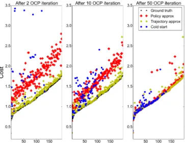
In the meantime, warm-start also results in more efficient trajectories. An important difference clearly appears in Fig. 6. The optimizer converges more quickly to the true optimum when initialized with the trajectory approximator ˆX∗
rather than by a roll-out of the policyπ. While the roll-out enforcesˆ
t=0.5s t=0.7s t=1.1s t=1.5s
t=1.5s t=1.9s t=2.4s t=2.9s
Fig. 7. snapshots of an example trajectory obtained with the predictive controller. At time 1.58s, the UAV is impacted by an object which suddently modifies its state. Using the initial guess, the predictive controller quickly reject the disturbance and converges to the desired equilibrium.
Fig. 6. Convergence of the predictive controller initialized either by the policy roll-out or by the trajectory approximation. We consider a fixed set of 200 initial points, for which the (global) optimal Value is known. The points are ordered by cost. We plot the cost obtained from the two approximations after 2, 10 and 50 iterations of the predictive controller. Initializing with the trajectory approximation, the solver quickly converges toward the optimal trajectory. Initializing with the policy rollout also leads the solver to a good solution, although 50 iterations are needed. In practice, when controlling a robot, we cannot afford more than 5 iterations.
the dynamic consistency, it also brings some convolution effects due to the dynamic instability, that tends to confuse the solver, at least during the first iterations. After a large number of iterations, both warm starts converge to the same optimum, with similar rate of failure.
The critical point with predictive control is to be able to quickly find an admissible trajectory. This is the case with both initial guess. However, on the robot, it is not possible to iterate more than 2 to 5 times. Under this assumption, the initialization by the trajectory approximator is much more efficient.
2) Predictive control: We use the initial guess in a pre-dictive controller. An example of the resulting trajectory is displayed in Fig. 7. The robot has to reached a desired steady state. During the movement, it is hit by an object: this impact instantaneously changes its velocity. A new trajectory is first approximated then optimized, leading the robot to reject the disturbance and to reach its final position.
TABLE I
SUCCESS RATE(%)OF THE STEERING METHOD AND AVERAGE COST(±
STANDARD DEVIATION)OF THE COMPUTED TRAJECTORIES FOR DIFFERENT WARM-START TECHNIQUES(U:WARM START FROM POLICY
ROLL-OUT, J:WARM START FROM STATE-CONTROL TRAJECTORY)AND AT DIFFERENT ITERATIONS(IT.)OF THE ALGORITHM.
U J Cold start
It. % Cost % Cost % Cost
2 90 0.47±0.18 88.5 0.07±0.07 31 2.05±1.85 5 90.5 0.34±0.10 93.5 0.07±0.08 45.5 0.37±0.36 50 85.5 0.04±0.09 85.0 0.03±0.07 42.0 0.06±0.10
Other trajectories are shown in the companion video (see https://youtu.be/CbyCa7aeC7k) with a dou-ble pendulum, a bicopter, a quadcopter in various situations and a quadcopter with swinging load. Snapshots from the videos are displayed in Figs. 8 to 11.
VI. CONCLUSION
This paper presented a new framework for the control of complex dynamical system. In particular, we addressed the open problem of providing a good initial guess to warm start a predictive controller. The proposed framework relies on sampling-based kinodynamic planning, trajectory optimization, and function approximation to compute and store the solution of a given optimal control problem. This solution is then efficiently retrieved online to warm start a predictive controller, thus speeding up its convergence.
Even though the presented results are preliminary, we believe that the proposed approach could scale to much higher-dimensional systems. This would unlock the so-far unexploited potential of predictive control on complex me-chanical systems.
REFERENCES
[1] T. P. Lillicrap, J. J. Hunt, A. Pritzel, N. Heess, T. Erez, Y. Tassa, D. Silver, and D. Wierstra, “Continuous control with deep reinforce-ment learning,” 2015.
[2] S. Levine and V. Koltun, “Guided Policy Search,” in International Conference on Machine Learning (ICML), vol. 28, 2013, pp. 1–9. [3] I. Mordatch and E. Todorov, “Combining the benefits of function
approximation and trajectory optimization,” Robotics: Science and Systems, 2014.
Fig. 8. Swings of a double pendulum to reach a desired upright position.
Fig. 9. Quadcopter trajectory from steady state to steady state. The controller is disturbed by an impact at the middle of the trajectory.
Fig. 10. Quadcopter trajectory from steady state to a waypoint with tilted angle (π/2) and nonzero velocity, then to a terminal steady state. The obstacle is not explicitely modeled in the control law.
Fig. 11. Quadcopter trajectory with a swinging load. The robot moves from steady state to steady state.
[4] I. Mordatch, N. Mishra, C. Eppner, and P. Abbeel, “Combining Model-Based Policy Search with Online Model Learning for Control of Physical Humanoids,” in IEEE International Conference on Robotics and Automation (ICRA), 2016.
[5] M. Zhong, M. Johnson, Y. Tassa, T. Erez, and E. Todorov, “Value function approximation and model predictive control,” in IEEE Sympo-sium on Adaptive Dynamic Programming and Reinforcement Learning (ADPRL), 2013, pp. 100–107.
[6] I. Lenz, R. Knepper, and A. Saxena, “DeepMPC: Learning Deep Latent Features for Model Predictive Control,” in Robotics: Science and Systems, 2015.
[7] A. Tamar, G. Thomas, T. Zhang, S. Levine, and P. Abbeel, “Learning from the Hindsight Plan – Episodic MPC Improvement,” in IEEE International Conference on Intelligent Robots and Systems (ICRA), 2017, pp. 336–343.
[8] M. Stolle and C. Atkeson, “Policies based on trajectory libraries,” in IEEE International Conference on Robotics and Automation, 2006, pp. 3344–3349.
[9] M. Bharatheesha, W. Caarls, W. J. Wolfslag, and M. Wisse, “Distance metric approximation for state-space RRTs using supervised learning,” in IEEE International Conference on Intelligent Robots and Systems, 2014, pp. 252–257.
[10] C. G. Atkeson, C. G. Atkeson, and C. Liu, “Trajectory-Based Dynamic Programming,” Modeling, Simulation and Optimization of Bipedal Walking Cognitive Systems Monographs, vol. 18, pp. 1–15, 2013. [11] D. H. Jacobson and D. Q. Mayne, “Differential dynamic
program-ming,” 1970.
[12] E. Todorov and W. Li, “A generalized iterative LQG method for locally-optimal feedback control of constrained nonlinear stochastic systems,” in American Control Conference (ACC), 2005.
[13] B. Houska, H. J. Ferreau, and M. Diehl, “Acado toolkitan open-source framework for automatic control and dynamic optimization,” Optimal Control Applications and Methods, vol. 32, no. 3, pp. 298–312, 2011. [14] I. Mordatch, E. Todorov, and Z. Popovi´c, “Discovery of complex behaviors through contact-invariant optimization,” ACM Transactions on Graphics, vol. 31, no. 4, pp. 1–8, jul 2012.
[15] M. Zhong, M. Johnson, Y. Tassa, T. Erez, and E. Todorov, “Value function approximation and model predictive control,” 2013 IEEE Symposium on Adaptive Dynamic Programming and Reinforcement Learning (ADPRL), pp. 100–107, 2013.
[16] A. Lucchi, Y. Li, and P. Fua, “Learning for structured prediction using approximate subgradient descent with working sets,” in IEEE Conference on Computer Vision and Pattern Recognition (CVPR), 2013, pp. 1987–1994.
[17] D. Kingma and J. Ba, “Adam: A method for stochastic optimization,” arXiv preprint arXiv:1412.6980, 2014.