HAL Id: hal-01976206
https://hal.laas.fr/hal-01976206
Submitted on 9 Jan 2019
HAL is a multi-disciplinary open access
archive for the deposit and dissemination of
sci-entific research documents, whether they are
pub-lished or not. The documents may come from
teaching and research institutions in France or
L’archive ouverte pluridisciplinaire HAL, est
destinée au dépôt et à la diffusion de documents
scientifiques de niveau recherche, publiés ou non,
émanant des établissements d’enseignement et de
recherche français ou étrangers, des laboratoires
Safe proactive plans and their execution
K. Madhava Krishna, Rachid Alami, Thierry Simeon
To cite this version:
K. Madhava Krishna, Rachid Alami, Thierry Simeon. Safe proactive plans and their execution.
Robotics and Autonomous Systems, Elsevier, 2006, 54 (3), pp.244-255. �hal-01976206�
Safe Proactive Plans and their Execution
K. Madhava Krishna
aR. Alami
bT. Simeon
ba: International Institute of Information Technology, Hyderabad - India b: LAAS-CNRS, 31077 Toulouse Cedex - France
Abstract: We present in this paper a methodology for computing the maximum velocity profile over a trajectory planned for a mobile robot. Environment and robot dynam-ics as well as the constraints of the robot sensors determine the profile. The planned profile is indicative of maximum speeds that can be possessed by the robot along its path with-out colliding with any of the mobile objects that could in-tercept its future trajectory. The mobile objects could be arbitrary in number and the only information available re-garding them is their maximum possible velocity. The ve-locity profile also enables to deform planned trajectories for better trajectory time. The methodology has been adopted for holonomic and non-holonomic motion planners. An ex-tension of the approach to an online real-time scheme that modifies and adapts the path as well as velocities to changes in the environment such that both safety and execution time are not compromised is also presented for the holonomic case. Simulation and experimental results demonstrate the efficacy of this methodology.
1
Introduction
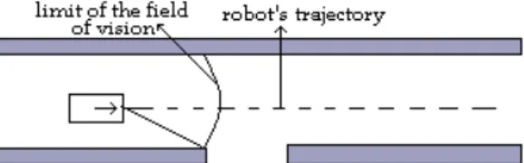
Several strategies exist for planning collision free paths in an environment whose model is known [9]. However during execution, parameters such as robot and environment dynamics, sensory capacities need to be incorporated for safe navigation. This is especially so if the robot navigates in an area where there are other mobile objects such as humans. For example in Figure 1, the robot would require to slow down as it approaches the doorway, in anticipation of mobile ob-jects to emerge from there, even if it does not intend to make a turn through the doorway.
A possible means to tackle the above problem at the execution stage is to always navigate the robot at very low speeds. In fact, reactive schemes such as the nearness diagram approach [11] operate the robot at minimal velocities throughout the navigation. How-ever incorporating the computation of a velocity pro-file at the planning stage would circumvent not only the problem of conservative velocities throughout nav-igation but would also allow for a modification of the trajectory to achieve lower time (Fig. 2).
Figure 1: A safe robot has to slow down while approaching the doorway
We present in this paper a novel pro-active strategy that incorporates robot and environment dynamics as well as sensory constraints into a collision free motion plan. By pro-active we mean that the robot is always in a state of expectation regarding the possibility of a mobile object impinging onto its path from regions in-visible to its sensor. This pro-active state is reflected in the velocity profile of the robot, which guarantees that in the worst case scenario, the robot will not col-lide with any of the moving objects that can interfere with its path. The ability of the algorithm to compute a-priori velocities for the entire trajectory accounting for moving objects moving in arbitrary directions is the essential novelty of this effort.
Figure 2: A longer path can be faster due to higher speed.
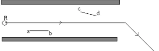
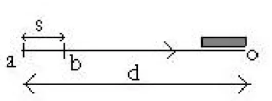
As is always the case, planned paths and profiles need constant modification at the execution stage due to changes in the environment. For example a profile and path that was planned for an environment with a closed doorway needs to be modified during real-time if the doorway is found open. Also addressed in this article the problem portrayed in Figure 3. Given an initial trajectory planned for a particular environ-ment how does the robot modify its trajectory while new objects (not necessarily intersecting the robot’s
trajectory) are introduced into the environment such that the basic philosophy of ensuring safety as well as reducing time lengths of the path continue to be respected. Simulation and experimental results are presented to indicate the efficacy of the scheme. In [1] we had reported how the maximum velocity profiles can be computed for any generic planner and in [8] we presented initial simulation and experimental results of the reactive version of [1].
Figure 3: How does the robot adapt its path in the pres-ence of new segments (a, b) and (c, d) while maintaining safe velocities?
Related work can be cited in the areas of modifying global plans using sensory data obtained during exe-cution for overcoming uncertainty accumulated during motions [3] and those that try to bridge the gap be-tween planning and uncertainty [10] or planning and control [7][2]. The velocity obstacle concept [13][5] bears resemblance to the current endeavor in that they involve selection of a robot velocity that avoids any number of moving objects. The difference is that in the present approach the only information about the mobile object available is the bound on velocity. The direction of motion and the actual velocities are not known during computation of the velocity profile. The work of Stachniss [14] also involves considering the robot’s pose and velocities at the planning phase. A path is determined in the (x, y) space and a subgoal is chosen. A sequence of linear and angular velocities, (v, w), is furnished till the subgoal is reached. In [12] a policy search approach is presented that projects a low dimensional intermediate plan to a higher dimensional space where the orientation and velocity are included. As a result better motion plans are generated that en-able better execution of the plan by the robot. The current effort has similarities to [12], at the planning level but also extends it to a suitable reactive level in the presence of new obstacles encountered during ex-ecution. Similarly the dynamic window approach [16] and the global dynamic window method of Brock et.al. [17] both incorporate the dynamics and the kinematics of the robot for a reactive collision avoidance system. Incorporating the dynamics and searching in the space of velocities overcome the problems of purely
geomet-ric methods. However these methods do not speak of modifying the path in order to reduce its time-length and the dynamics of the environment does not affect the computation of the velocity profile, which places our approach as different from those mentioned above.
2
Problem Definition
The following problems are addressed in the paper, given:
• A robot R modelled as a disc and equipped with an omnidirectional sensor having a limited range Rvis. We call Cvisthe visibility circle, centered at
robot’s position with radius Rvis. The paths of
R are sequences of straight segments or straight segments connected with circular arcs of radius ρ in case of a non-holonomic robot. The robot’s motion is subject to dynamic constraints simply modelled by a bounded linear velocity v ∈ [0, vrm]
and a bounded acceleration a ∈ [−a−m, am]. The
maximum possible deceleration a−m need not
equal the maximum acceleration am.
• A workspace cluttered by static polygonal obsta-cles Oi. The static obstacles can hide possible
mobile objects whose motions are not predictable; the only information is their bounded velocity vob.
Problem 1: Given a robot’s path τ (s) computed by a standard planner [9], determine the maximal veloc-ity profile vτ(s) such that, considering the constraints
imposed by its dynamics, the robot can stop before collision occurs with any of the mobile objects that could emerge from regions not visible to the robot at position s ∈ τ (s). For example the velocity profile dictates that the robot in Figure 1 slow down near the doorway in expectation of mobile objects from the other side. We call M P = (τ (s), vτ(s)) a robust
mo-tion plan. The velocity profile allows us to define the time T (τ ) required for the robust execution of path τ :
T (τ ) = Z L
0
ds vτ(s)
Problem 2: Modify the planned trajectory such that the overall trajectory time T (τ ) is reduced. For example, the path of Figure 2, albeit longer than the one of Figure 1 is traversed in a shorter time.
Problem 3 Adapt the path and velocities reactively in the presence of new objects not a part of the original workspace such that the criteria of safe velocities and reduced time of path continue to be respected. This is illustrated in Figure 3.
3
From path to robust motion plan
The procedure for computing the maximum veloc-ity profile vτ(s) delineated in Sections 3.1, 3.2 and
3.3 addresses the first problem. The constraints im-posed by the environment on the robot’s velocity are due to two categories of mobile objects. The first cate-gory consists of mobile objects that could appear from anywhere outside the boundary of the visibility cir-cle Cvis. The second category involves mobile objects
that could emerge from shadows created in Cvis due
to stationary objects.
3.1
Velocity constraints due to the
envi-ronment
C
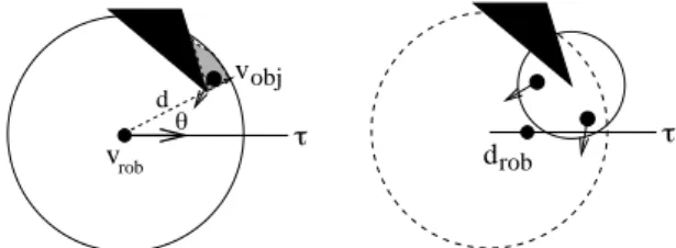
vis v(0) = vrob v(t )=00 dobj drob vobj v(t)= v -a trob m vrobFigure 4: Mobile objects may appear anywhere on Cvis’s
contour.
No obstacles in Cvis In the simple case where the
robot’s position is such that no static obstacle lies in-side Cvis, a moving object may appear (at time t = 0)
anywhere on Cvis’s boundary (Fig. 4). Let Vrb denote
the maximum possible robot velocity due to a mobile object at the boundary. At time t0 = vrb/a−m (i.e.,
when the robot is stopped), the distance crossed by the object is dobj(vrb) ≤ vobvrb/a−m. Avoiding any
poten-tial collision imposes that Rvis≥ drb(vrb) + dobj(vrb),
where drb = vrb2/2a−m. The condition relates vrb to
the sensor’s range Rvis as:
vrb= −vob+
q v2
ob+ 2a−mRvis (1)
Influence of shadowing corners Static obstacles lying inside Cvismay create shadows (e.g., see the grey
region of Figure 5) which contain mobile objects. The worst-case situation occurs when the mobile object re-mains unseen until it arrives at the shadowing corner of a polygonal obstacle. Since the mobile object’s mo-tion direcmo-tion is not known it is best modeled for a worst case scenario as an expanding circular wave of radius vobt centered at (d, θ)
(X(t) − d cos θ)2+ (Y (t) − d sin θ)2= v2obt2
Let us first consider that the robot’s path τ is a straight segment. Considering that the intersections between the circular wave and the robot’s segment path, should never reach the robot before it stops at time t0 = vrs/a−m yields the following velocity
con-straint: vrsv4 − 4(a−md cos θ + v2ob)v 2 rsv+ 4a 2 −md2≥ 0 (2)
Here vrsv is the maximum possible robot velocity due
to the shadowing vertex under consideration. The so-lution of Eq. 2 gives vrsv, as a function of (d, θ).
drob vobj rob v d θ τ τ
Figure 5: Mobile objects may also appear from the shad-ows of static obstacles
This solution only exists under the condition vob>
pa−md(1 − cos θ), i.e., when the object’s velocity vob
is sufficiently high to interfere with the robot’s halt-ing path. Otherwise, the shadowhalt-ing corner does not constrain the robot’s velocity which can be set to vrm,
the maximum bound on robot’s velocity.
Similar reasoning can be applied to the case where the robot traverses a circular arc path of radius ρ. This case however leads to a nonlinear equation that needs to be solved numerically to derive the maximal velocity [4]. The expression that needs to be solved for computing the maximum velocity at a given point on a circular arc is of the form :
((v2rsvv2ob)/a−m2 ) + 2ρ2cos(v2ob/2a−mρ)+
2dρ sin((vob2/2a−mρ) − θ)
= d2+ 2ρ2− 2dρ sin θ (3)
3.2
Computing the shadowing corners
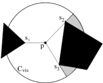
The problem of determining the set of shadowing corners needed for the velocity computation in Sec-tion 3.1 is the problem of extracting those vertices of the polygonal obstacle to which a ray emitted from the robot’s center is tangential (Figure 6). The set of shadowing corners can be easily extracted from an algorithm that outputs the visibility polygon [15] as a sorted list of vertices.
C s s s vis 1 2 3 p
Figure 6: Shadowing corners: among the three vertices of V(p), only s2and s3create shadows (the line going through
s1 is not tangent to the left obstacle).
3.3
Computing the velocity profile v
τ(s)
While the methodology for computing the maxi-mum velocity profile delineated here is essentially for a holonomic path, its extension to the non-holonomic case is not very difficult.
1. A holonomic path τ , consisting of a sequence of straight line segments ab, bc, cd (Fig. 7) is deformed into a sequence of straight lines and clothoids to ensure continuity of velocities at the bends [6]. The maximum deviation from an end-point to its clothoidal arc (depicted as e in Figure 7) is dependent on the nearest distance to an ob-ject from the endpoint under consideration.
Figure 7: A holonomic path deformed into a sequence of straight segments and clothoidal arcs.
2. The linear velocity along a clothoid is a constant and the maximum possible linear velocity consid-ering robot dynamics alone is calculated for each of the clothoidal arc a1b0, b1c0 according to [6] and is represented as vc(a1), vc(b1).
3. The straight segment aa1 is discretized into M equally spaced points, excluding the endpoints of the segment, viz. a and a1. We denote the first such point as a1 and the last such point as aM.
The point of entry into the clothoid, viz. a1 is also denoted as aM +1.
4. For each of the N points, ai, the steps 4a to 4e
are repeated.
4a Maximum possible velocity that a robot could have such that it can come to a halt before collid-ing with objects that enter into the robot’s field of
vision from the boundary is computed as vrb(ai)
according to Equation 1.
4b Velocity of the robot due to stationary obstacles inside the robot’s field of vision that create shad-ows is computed as vrsv(ai) according to
Equa-tion 2. The minimum of all the velocities due to such vertices is found and denoted as vrs(ai).
4c The maximum possible velocity of the robot at ai
due to environment is then computed as
vre(ai) = min(vrb(ai), vrs(ai)) (4)
4d Velocity of the robot at aidue to its own
dynam-ics is given by vrd(ai) =
p v2
r(ai−1) + 2ams(ai, ai−1) (5)
The above equation is computed if vre(ai) >
vr(ai−1). Here s(ai, ai−1) represents the distance
between the points ai and ai−1. am represents
the maximum acceleration of the robot. 4e The eventual velocity at ai is given by
vr(ai) = min(vrd(ai), vre(ai), vrm) (6)
Here vrm represents the maximum robot velocity
permissible due to servo motor constants. 5. The velocity at the endpoint a1 is computed as
vr(a1) = min(vr(a1), vc(a1)) and this would be
the linear velocity with which the robot would traverse the clothoid.
6. Steps 6a and 6b are performed by going back-wards on each of the N points from aN to a1.
6a If vr(ai) > vr(ai+1) then the modified maximum
possible velocity at ai is computed as
vrd(ai) =
p v2
r(ai+1) + 2a−ms(ai, ai+1) (7)
6b Finally the maximum safe velocity at ai is given
as vr(ai) = min(vr(ai), vrd(ai)).
7. Repeat steps 3 to 6 for all the remaining straight segments to obtain the maximal veloc-ity profile over a given trajectory τ as vτ(s) =
{vr(a), vr(a1), ..., vr(aN), vr(a1), vr(b1), ..., vr(d)}.
3.4
Modifying
planned
trajectory
for
lower time
The knowledge of the maximum velocity profile over a trajectory is utilized to tackle the problem posed in Section 2 of reducing the overall trajectory time of the path. The procedure for reducing trajectory time at the planning stage involves random deformation of the planned path and evaluating time along this path. The modified path becomes the new trajectory if time
along it is less than along the original trajectory. The process is continued till over a finite number of at-tempts no further minimization of trajectory time is possible. Prior to delineating the algorithm it is to be noted that the set of all collision free space of the workspace is denoted as Cf ree and the current
trajec-tory of the robot as τc(s). A point of discretization
on a trajectory discretized into N parts is denoted as p(si), i ∈ {1, 2, ..., N }. The corresponding
configura-tion of the robot at those points is denoted by q(si).
The algorithm is given as Algorithm 1.
Algorithm 1 Globally reducing trajectory time
1: Ntry ← 0
2: while Ntry < Nattempts do
3: Discretize current trajectory τc(s) into Npparts
where Np is selected based on minimum
dis-cretization distance between two points.
4: Set f lag ← 0
5: for i = 1 to Npdo
6: Compute minimum velocity at sidue to
shad-owing vertices as vrmin(si)
7: if vrmin(si) < vrm then
8: Find a configuration q(sp) ∈ Cf ree and
sp ∈ τ/ c(sk), k ∈ {1, ..., Np} such that q(sp)
is reachable from q(si).
9: Find a point sr on the remaining part of
the trajectory, sr∈ τc(sj); i < j ≤ Np such
that q(sr) is reachable from q(sp).
10: Form a new trajectory through si, sp, sq
and denote it as τn(s)
11: if T (τn) < T (τc) then
12: discretize τn into Nq points.
13: τc← τn 14: Np← Nq 15: Set f lag ← 1 16: end if 17: end if 18: end for 19: if f lag = 0 then 20: Ntry← Ntry+ 1 21: end if 22: end while
Step 8 of the algorithm is carried out by searching for a collision free configuration which would displace the path away from the shadowing vertex responsible for the lowest velocity at si . Step 11 adapts the
dis-placed path as the new current path if its trajectory time is less than the current path. Nattempts, is the
number of unsuccessful attempts at minimizing tra-jectory time before the algorithm halts.
3.5
Remembering Sensor Information
The computation of the velocity profile at a given point on the robot’s trajectory incorporates the robot’s field of vision at that point. This field can change appreciably between two successive instances of computation. For example in Figure 8 the robot at position a has full field of vision of the corridor that is transverse to the robot’s trajectory. However at posi-tion b the robot is blind to the zone shown in darker shade of gray. Hence it needs to slow down as it moves further down to c since it envisages the possibility of a moving object approaching it from the corners of the stationary objects. These corners are the starting areas of the robot’s blindzone at b.
Figure 8: Memorization of previous scenes
However, if the robot could remember the earlier scene it could use this when computing its velocity profile during execution of the planned path. In such a case, if the robot did not see any moving objects in close proximity at a it can make use of this information at b to have a velocity profile from b that is greater than the one computed in the absence of such infor-mation. Figure 8 shows (in darker shade) the zone remembered by the robot. The contour of the remem-bered area represents the blindzone of the robot at b, from where mobile objects can emanate. The area in lighter shade of gray is the visibility polygon for the robot at b. With the passage of time the frontier of the remembered area shrinks due to the advancement of the imagined mobile objects from the initial frontier. The details of this scheme are given below.
Remembering is fruitful when a non-shadowing ver-tex begins to cast a shadow thereby hiding regions which were previously visible. The set of all
ver-Figure 9: Three categories of blind vertices.
tices that are currently visible, shadowing and were at some prior instant visible, non-shadowing is denoted by V sns. For every vertex ve ∈ V sns a correspond-ing vertex is associated and called the blind vertex. The blind vertices are of three categories explained in Figure 9 where the vertex a, non-shadowing for the robot at p becomes shadowing when the robot is at q. Correspondingly the vertex c of the triangular obsta-cle which was visible and shadowing when the robot was at p becomes invisible when the robot moves to q. Simultaneously one of the other end-points of a, viz. b, would also become inevitably invisible at q. Ver-tices like b fall in the second category. If b was already outside Cvisat p the intersection of Cviswith the
seg-ment ab, namely o is identified as the third category of blind vertex. The set of all such vertices is denoted by V bs. These vertices are advanced by a distance vob∆t
where ∆t is the time taken by the robot between p and q to new virtual locations along the line that connects those vertices to a. At q the velocity is computed due to the closest of the vertices in the set V bs at their virtual locations instead of a, which is otherwise the vertex for which equation(2) is computed.. Such a trend continues till the distance between the robot to the closest hypothetical vertex is less than the actual distance of the robot to a.
The remembering part of the algorithm is given in algorithm 2. The set of all visible shadowing vertices is denoted by V sh.
4
From Plan to Execution
The velocity profile, vτ(s), is a sequence of
max-imum velocities calculated at discretized locations along the trajectory τ (s). The locations at which the velocity profile at the execution stage is computed are not the same locations as where the profile was com-puted during planning, due to odometric and motor
Algorithm 2 Remembering effects on velocity
1: for each vertex ve∈ V sh do
2: if ve∈ V sns then
3: for each vertex vb ∈ V bs associated with ve
do
4: Advance vb by vob∆t
5: end for
6: Denote the distance from the robot’s current location, sc, to the closest of all advanced
ver-tices, vbc as dcvb
7: if d(sc, ve) < dcvb then
8: Compute velocity due to the virtual vertex vbcthrough Equation 2
9: else
10: Compute velocity due to the actual vertex vethrough Equation 2
11: end if
12: end if
13: end for
constraints. Moreover, if there are changes in the envi-ronment it entails modifying the trajectory and hence the velocities. During execution it is computationally expensive to compute the profile for the entire remain-ing trajectory, hence the profile is computed for the next finite distance, given by, dsaf e= dmax+ ndsamp,
where dmax= vrm2 /(2 ∗ a−m), represents the distance
required by the robot to come to a halt while it moves with the maximum permissible velocity afforded by motor constants. And dsamp = vrmtsamp is the
max-imum possible distance that the robot can move be-tween two successive samples (time instants) of trans-mitting motion commands, where time between two samples is tsamp.
The main issue here is what should be the distance over which the velocity profile needs to be computed during execution such that it is safe. A velocity com-mand is not considered safe if it is less than the cur-rent velocity and not attainable within the next sam-ple. The velocity is constrained by the environment as well as robot’s own dynamics and hence their roles are studied below.
Effect of Environment Mobile objects that can emerge from corners in a head-on direction cause the greatest change in velocity over two samples. Figure 10 shows one such situation, where the rectangular object casts a shadow and is susceptible to hide mobile objects. Let the current velocity of the robot at a due to the object be v1. Let the velocity at a distance, s,
Figure 10: Effect of an obstacle on the robot’s velocity, possibly hiding mobiles objets at locations a and b.
The velocities at a and b are given by
va= −vob+ q v2 ob+ 2a−md (8) vb= −vob+ q v2 ob+ 2a−m(d − s) (9) Hence va2− vb2= 2a−ms+ 2vob( q v2 ob+ 2a−m(d − s) − q v2 ob+ 2a−md) (10)
Evidently the second term on the right hand side of Equation 10 is negative, since the second square root term is more positive than the first. Hence v2
a− v2b ≤ 2a−ms. Therefore the velocity at b, vb can
be attained from the velocity at a, va under
maxi-mum deceleration, dm, irrespective of the maximum
velocity of the mobile object or the robot’s own motor constraints. This was intuitively expected since the robot’s velocity at any location is the maximum pos-sible velocity that guarantees immobility before colli-sion; its velocity at a subsequent location permitted by the environment would be greater than or equal to the velocity at the same location obtained under maximum deceleration from the previous location. In other words for safeness of velocity going purely by environmental considerations it would suffice to calcu-late the velocity, for the next sampling distance alone, for without loss of generality, d = dsamp.
Effect of robot’s dynamics The robot needs to respect the velocity constraints imposed while near-ing the clothoidal arcs and eventually while comnear-ing to the target. The robot can reach zero velocity from its maximum velocity over a distance of dmax, computed
before. Hence dmax+ dsamp represents the safe
dis-tance over which the velocities need to be computed.
4.1
Online path adaptation for better
tra-jectory time
The third of the problems outlined in Section 2 is tackled here. During navigation the robot in general comes across objects hitherto not a part of the map.
The robot reacts to these new objects in line with the basic philosophy of safety as well as time reduced paths. The adaptation proceeds by finding locations over a finite portion of the future trajectory where drops in velocity occur and pushing the trajectory away from those vertices of the objects that caused these drops to areas in free space where higher veloci-ties are possible. A search is made through the newly found locations of higher velocities for a time reduced path.
Generalized Procedure The generalized proce-dure for adapting the path in the presence of new objects is delineated through Figure 11.
Figure 11: A trajectory in the presence of new ob-jects. The points marked with crosses represent locations through which a path is searched for reduced time of tra-jectory.
1. On the trajectory segment that is currently tra-versed, AB in Figure 11, enumerate the vertices of objects that reduce the velocity of the robot. 2. The positions are found on AB where the
influ-ence of vertices is likely to be maximal.
3. These positions are pushed by distances dp =
k(vl− vr), where vl and vr are the velocities at
that location on the path due to the most influ-ential vertices on the left and right of the path. These new locations are denoted as p1, p2, p3, p4 (Fig.11) and maintained as a list provided the ve-locity at the new locations is higher than the orig-inal ones. p6 is the farthest point on the robot’s trajectory visible from its current location at A. 4. On this set of locations A, p1, p2, p3, p4, p5, p6
starting from the current location at A, find a trajectory sequence shorter in time than the cur-rent sequence of A, B, p6 if it exists.
5. The steps 1 to 4 are repeated until the robot reaches the target.
It should be noted that when a collision with an ob-ject is detected, a collision free location is first found that connects the current location with another loca-tion on the original trajectory and this new collision
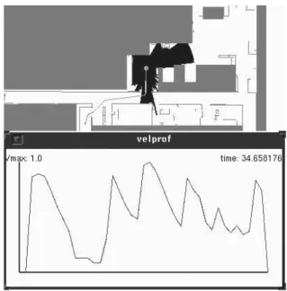
Figure 12: Path computed by a typical planner and its velocity profile shown on the top. The robot’s velocity corresponding to its location on the trajectory is shown by a vertical line on the profile and labeled as m.
free path is further adapted for a time-reduced path if it exists. Also note that while the velocities are com-puted over a distance dsaf e, that part of the remaining
trajectory that is visible from the current location is considered for adapting to a better time-length.
5
Planning Results and Analysis
In this section the results of incorporating the ve-locity profile computation as a consequence of con-sidering robot and environment dynamics and sensor capacities at the planning stage and the subsequent adaptation of paths to better time of trajectory is ana-lyzed. Figure 12 shows the path computed by a typical holonomic planner [9] and its corresponding velocity profile. The velocity corresponding to the robot’s lo-cation on the trajectory (shown as a small circle) is marked by a straight line labeled m on the profile. The dark star-shaped polygon centered at the robot depicts the visibility of the robot at that instant and is called the visibility polygon. The figure is a snap-shot of the instant when the robot begins to decelerate to a velocity less than half the current velocity as it closes down on the vertex a marked in the figure. Evi-dently from the visibility polygon the vertex a casts a shadow and the closer the robot gets to it, the slower the velocity must be.
Figure 13 is the time reduced counterpart of Figure 12. The snapshot is once again at a location close to vertex a. Staying away from a permits nearly max-imum velocity. The dip observed in the profile due to vertex a is negligible. Similarly staying away from other vertices such as b allows for a trajectory time of 21.79s compared to 26.30s for Figure 12.
Mod-Figure 13: Path obtained after adaptation to reduced time-length.
ification of the trajectory for shorter time proceeds along the lines of Section 3.4. For the two examples discussed, the robot’s maximum acceleration and de-celeration was fixed at 1m/s2, maximum velocity at 1m/s and the sensor range at 7m. The maximum bound on the object’s velocities was 1.5m/s.
Figures 14 and 15 depict the planned trajectory and velocity profiles before and after reduction of trajec-tory time for our laboratrajec-tory environment. The time reduced trajectory is shorter by more than 8 seconds as it widens its field of view by moving away from the bends while turning around them.
Figure 14: Planned trajectory before adaptation to a re-duced time.
Figure 15: Time reduced trajectory at planning stage.
5.1
Effect of remembering on trajectory
time
Figure 16 shows an environment with four corridors named 1, 2, 3 and 4 with planned path obtained by minimizing time. It also portrays the robot’s field of vision as it enters corridor 3. The velocity profile for the above path is shown in Figure 17. The location of the robot corresponding to its location in Figure 16 is shown through the vertical line. The locations of the robot as it decelerates when its field of view of each of the corridors vanishes is also marked with the respective numbers on the profile.
Figure 16: Robot’s field of view as it enters corridor 3.
Though the path of Figure 16 is minimized in time its velocity profile still shows decelerations in the vicin-ity of the corridors. This is due to the phenomenon discussed in Section 3.5 where the robot becomes blind to many parts of the environment it had seen at the preceding instant. Figure 18 shows the robot’s field
of vision at an instant after the one shown in figure 16. There is a marked decrease in its field of vision at the latter instant that results in the robot reducing its velocity in anticipation of moving objects from the blindzones depicted in the velocity profile.
Figure 17: Velocity profile for the Figure 16. Correspond-ing position of the robot shown in vertical line. Deceler-ations near the corridors are also marked with the same numbers.
Figure 18: Robot’s field of vision at an instant that im-mediately follows the instance of Figure 16.
Figure 19: Velocity profile obtained after incorporation of memory
However, when the robot is able to remember the previous images, the need to decelerate is nullified and the trajectory time is further reduced. Figure 19 il-lustrates this where the decelerations shown in the ve-locity profile of Figure 17 at locations 1, 2, 3 and 4 are now absent.
Figure 20: A simple planned trajectory and its velocity profile.
6
Experimental Results
6.1
Velocity profiles
In this section the velocity profiles obtained dur-ing the planndur-ing and execution stages are compared in the absence of any new objects during execution. Figure 20 shows a simple planned trajectory and the corresponding velocity profile for our lab environment. Some of the obstacles are filled in gray and others are shown as segments (in gray). The robot is shown as a small circle and the star shaped polygon in black rep-resents the field of vision of the robot at that location. The vertical line, marked m in the velocity profile rep-resents the velocity of the robot corresponding to its position on the trajectory. The profile shows a subse-quent drop in velocity, a consesubse-quent of robot getting closer to region marked, d, to which it is blind.
Figure 21 compares the planned and executed (in simulation) velocity profile. The executed trajectory tallied to a time of 12.28s in comparison with 12.25s for the planned profile. These figures illustrate that the executed profiles and execution times are close to the planned profiles and times while there are no changes in the environment.
Figures 23 and 24 show the execution by the Nomad XR4000 (Fig. 22) of paths computed by a standard planner. Figure 23 corresponds to the original path computed by the planner and Figure 24 is its time reduced counterpart.
The velocity profiles during execution of the two
Figure 21: The planned and executed velocity profile in simulation. The ordinate measures velocity in m/s and abscissa time in seconds.
Figure 22: The Nomad XR4000 used in our experiments at LAAS.
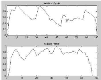
paths are shown in Figure 25. Some of the bigger drops in the unreduced profile are absent in the re-duced profile as the robot avoids turning close to the obstacles that form the bends. The path of Figure 24 got executed in 12.9s while the path in Figure 23 was executed in 13.98s. The Figures are meant as illustrations of the theme that trajectories deformed to shorter time-lengths at planning stage are also ex-ecuted in shorter time during implementation than their unreduced versions.
Figure 23: Execution of the original planned path.
Figure 24: Execution of the time-reduced path.
6.2
Online adaptation of paths for better
trajectory time
This section presents results of the algorithm in the presence of newly added objects that affect the ve-locities of the robot in real-time. Figure 26 shows a path where the robot avoids the two new segments S1 and S2 intersecting the original planned trajectory but does not adapt its path for better time. The velocity profile for the same is shown in Figure 27. Figure 28 is the counterpart of Figure 29 where the robot adapts its path to a better time-length reactively. The big dips in the velocity profile of Figure 27 are filtered in Figure 29 considerably as the robot avoids the ob-stacles with larger separation. The time reduced ex-ecution tallied to 10.9s while the unreduced version was executed in 12.5s. The trajectory time at plan-ning was 7.9s. The above graphs are those obtained in simulation.
Figure 25: The top profile corresponds to the path ex-ecuted in Figure 23 and the bottom to Figure 24. The planned and executed velocity profile in simulation. The ordinate measures velocity in m/s and abscissa time in seconds.
Figure 26: A simulated execution in the presence of two new segments S1 and S2 along with the corresponding velocity profile. The path is not adapted to better time-length. Start and goal locations marked as S and T .
Figure 30 shows the unreduced executed path by the XR4000 Nomadic robot in our laboratory at LAAS. The obstacles in the original map are shown by black lines, while the segments perceived by the SICK laser are shown in lighter shades of gray. Some of these segments get mapped to the ones in the map and the others are considered new segments. This is done by a segment based localization algorithm. The segments of concern here are those which form a box shaped obstacle marked B in Figure 30. The vertex d of this
Figure 27: Velocity profile for the execution of Figure 26.
Figure 28: Path of Figure 26 adapted to better time-length.
obstacle casts a shadow on the robot’s sensory field, which forces it to slow down at those locations due to Equation 2. The execution time for this unreduced path is 10.6s.
The time reduced counterpart is shown in Figure 31 that tallied to 9.6s. The original planning time was 8.8s in the absence of the box shaped object. The corresponding velocity profile is shown in figure 32.
7
Conclusions and Scope
A proactive safe planning algorithm and its reac-tive version that facilitates real-time execution has been presented. The proactive nature of the
algo-Figure 29: Velocity profile for the execution of Figure 28.
Figure 30: Unreduced path executed by the Nomad XR4000. The vertex d of the new box shaped object B forces a slow down near it.
rithm stems from the computed velocity profile, vτ(s),
that guarantees immobility of the robot before colli-sion with any of the possible mobiles that could inter-fere its future trajectory from regions blind to its sen-sor. The proactivity does not however come at the cost of robot’s velocity or trajectory time. The knowledge of vτ(s) computed over the trajectory τ (s) further
fa-cilitates reduction of the over all trajectory time T (τ ) by adaptation of the initially planned path. Analy-sis of the scheme at the planning stage depict that the robot can have a velocity profile that achieves its max-imum possible velocity for a sustained duration with-out many dips provided it stays away from doorways
Figure 31: Time reduced path executed by the Nomad XR4000.Increasing linear and angular separation from ver-tex d facilitates a higher speed.
Figure 32: Velocity profile for the path executed by the Nomad in Figure 31. The planned and executed velocity profile in simulation. The ordinate measures velocity in m/s and abscissa time in seconds.
and narrow passages along its path. Remembering of previous scenes also enhances the robot’s performance through reduced trajectory time and a more uniform velocity profile.
A reactive extension of the scheme that facilitates real-time simulation and implementation is also pre-sented. The scheme maintains the underlying philos-ophy of computing safe velocities and modification of paths for better trajectory time. Simulation and ex-perimental results at real-time corroborate our earlier results obtained at the planning stage (that by keep-ing away from vertices of objects that could hide mo-biles the robot could move at higher velocities and obtain better time-lengths) and thus the efficacy of
overall strategy is vindicated. The minimum distance over which the velocities need to be computed on the remaining trajectory during real-time such that the computed velocities are safe is theoretically es-tablished. This avoids repetitive computation of ve-locities over the entire remaining trajectory for every motion command, thereby reducing computational in-tensity and facilitating for real-time implementation. The methodology could be useful in the context of per-sonal robots moving in areas where interference with mobile humans especially aged ones are generally ex-pected.
Immediate scope of this work involves in incorpo-rating the memory phenomena at the reactive level such that higher speeds are possible. The method-ology needs to be validated in the presence of mo-bile objects that actually impinge on the path from blindzones with a provision for the robot to avoid the objects without halting, continuing to respect safety considerations as well as minimizing trajectory time.
Acknowledgments
The work described in this paper was conducted within the EU Integrated Project COGNIRON (”The Cognitive Companion”) and was funded by the Eu-ropean Commission Division FP6-IST Future and Emerging Technologies under Contract FP6-002020 and by the French National Program ROBEA.
References
[1] R. Alami, T. Sim´eon, and K.Madhava Krishna. On the influence of sensor capacities and en-vironment dynamics onto collision-free motion plans. IEEE/RSJ International Conference on Intelligent Robots and Systems, EPFL, Swizer-land, 2002.
[2] J.C. Alvarez, A. Skhel, and V. Lumelsky. Ac-counting for mobile robot dynamics in sensor-based motion planning: experimental results. IEEE International Conference on Robotics and Automation, Leuven (Belgium), 1998.
[3] B. Bouilly, T. Sim´eon, and R. Alami. A numeri-cal technique for planning motion strategies of a mobile robot in presence of uncertainty. IEEE In-ternational Conference on Robotics and Automa-tion, Nagoya (Japan), 1995.
[4] D. Cruzel. Planification de mouvements sous con-traintes de perception. Master’s thesis, LAAS-CNRS, 1998.
[5] P. Fiorinin and Z. Schiller. Motion planning in dynamic environments using velocity obsta-cles. International Journal of Robotics Research, 17(7):760–772, 1998.
[6] S. Fleury, P. Soueres, and J.P. Laumond. Prim-itives for smoothing mobile robot trajectories. IEEE Transactions on Robotics and Automation, 11(3):441–448, 1995.
[7] M. Khatib, B. Bouilly, T. Sim´eon, and R. Chatila. Indoor navigation with uncertainty using sensor-based motions. IEEE International Confer-ence on Robotics and Automation, Albuquerque (USA), 1997.
[8] K.Madhava Krishna, R. Alami, and T. Sim´eon. Moving safely but not slowly - reactively adapting paths for better trajectory times. IEEE Interna-tional Conference on Advanced Robotics, Quim-bra, Portugal, 2003.
[9] J.C. Latombe. Robot Motion Planning. Kluwer Academic, 1991.
[10] A. Lazanas and J.C. Latombe. Motion planning with uncertainty: a landmark approach. Artificial Intelligence, pages 287–315, 1995.
[11] J. Minguez and L. Montano. Nearness diagram navigation. a new real-time collision avoidance approach. IEEE/RSJ International Conference on Intelligent Robots and Systems, 2000.
[12] N. Roy and S. Thrun. Motion planning through policy search. IEEE/RSJ International Confer-ence on Intelligent Robots and Systems, EPFL, Swizerland, pages 2419–2425, 2002.
[13] Z. Schiller, F. Large, and S. Sekhavat. Motion planning in dynamic environments: Obstacles moving along arbitrary trajectories. IEEE In-ternational Conference on Robotics and Automa-tion., pages 3716–3721, 2001.
[14] C. Stachniss and W. Burgard. An integrated ap-proach to goal-directed obstacle avoidance un-der dynamic constraints for dynamic environ-ments. IEEE/RSJ International Conference on Intelligent Robots and Systems, EPFL, Swizer-land, 2002.
[15] S. Suri and J. O’Rourke. Worst-case optimal al-gorithms for constructing visibility polygons with holes. ACM Symp. on Computational Geometry, 1986.
[16] D Fox, W Burgard and S Thrun The Dynamic Window Approach to Collision Avoidance IEEE Robotics and Automation Magazine, 1997. [17] Brock, Oliver and O Khatib High Speed
Navigation using the Global Dynamic Window Approach IEEE International Conference on Robotics and Automation, 1997.