Communication theory of quantum systems.

4/

RESEARCH LABORATORY OF LECTRONICS MASSACHUSETTS INSTITUTE OF TECHNOLOGY

I

COMMUNICATION THEORY OF QUANTUM SYSTEMS

HORACE P. H. YUEN

LOAN

c

COPY

TECHNICAL REPORT 482

AUGUST 30, 1971

MASSACHUSETTS INSTITUTE OF TECHNOLOGY RESEARCH LABORATORY OF ELECTRONICS

The Research Laboratory of Electronics is an interdepartmental laboratory in which faculty members and graduate students from numerous academic departments conduct research.

The research reported is this document was made possible in part by support extended the Massachusetts Institute of Tech-nology, Research Laboratory of Electronics, by the JOINT SER-VICES ELECTRONICS PROGRAMS (U. S. Army, U. S. Navy, and U. S. Air Force) under Contract No. DA 28-043-AMC-02536(E),

and by the National Aeronautics and Space Administration (Grant NGL 22-009-013).

Requestors having DOD contracts or grants should apply for copies of technical reports to the Defense Documentation Center, Cameron Station, Alexandria, Virginia 22314; all others should apply to the Clearinghouse for Federal Scientific and Technical Information, Sills Building, 5285 Port Royal Road, Springfield, Virginia 22151.

THIS DOCUMENT HAS BEEN APPROVED FOR PUBLIC RELEASE AND SALE; ITS DISTRIBUTION IS UNLIMITED.

--MASSACHUSETTS INSTITUTE OF TECHNOLOGY RESEARCH LABORATORY OF ELECTRONICS

Technical Report 482 August 30, 1971

COMMUNICATION THEORY OF QUANTUM SYSTEMS

Horace P. H. Yuen

Submitted to the Department of Electrical Engineering at the Massachusetts Institute of Technology in June 1970 in partial ful-fillment of the requirements for the degree of Doctor of Philosophy.

(Manuscript received January 1, 1971)

THIS DOCUMENT HAS BEEN APPROVED FOR PUBLIC RELEASE AND SALE; ITS DISTRIBUTION IS UNLIMITED.

Abstract

The primary concern in this research is with communication theory problems in-corporating quantum effects for optical-frequency applications. Under suitable con-ditions, a unique quantum channel model corresponding to a given classical space-time varying linear random channel is established. A procedure is described by which a proper density-operator representation applicable to any receiver configuration can be constructed directly from the channel output field. Some examples illustrating the application of our methods to the development of optical quantum channel representa-tions are given.

Optitnizations of communication system performance under different criteria are considered. In particular, certain necessary and sufficient conditions on the optimal detector in M-ary quantum signal detection are derived. Some examples are presented. Parameter estimation and channel capacity are discussed briefly.

ii

TABLE OF CONTENTS

Part I. DEVELOPMENT OF COMMUNICATION SYSTEM MODELS

A. GENERAL INTRODUCTION AND SUMMARY OF PART I 1

1. 1 Summary of Part I 2

1.2 Relation to Previous Work 2

1.3 Nature of our Theory 3

1.4 Background 4

1.5 Outline of Part I 4

B. CLASSICAL RANDOM FIELD PROPAGATION AND

COMMUNICATION SYSTEMS 6

2. 1 Partial Differential Equation Representation of

Channels 6

2. 1. 1 General Case 8

2. 1. 2 Markov Case 12

2. 1. 3 Stationary Case 17

2.2 Nondifferential Filter Channels 18

2.3 System Normal and Noise Normal Modes 19

2.4 Stochastic Channels 21

2. 4. 1 Random Green's Function 21

2. 4. 2 Stochastic Normal Modes 22

2. 5 Stochastic Signals 24

2.6 Relation to Ordinary Filter Description 25

2.7 Conclusion 27

C. QUANTUM RANDOM PROCESSES 28

3. 1 Quantum Probabilistic Theory 28

3. 1. 1 Self-adjoint Quantum Variables 29

3. 1. 2 Non-Hermitian Quantum Observables 29 3. 1. 3 Quasi Densities and Characteristic Functions 32

3. 1.4 Gaussian Quasi Variables 34

3. 1. 5 Statistically Independent Quasi Variables 37 3. 1. 6 Sums of Independent Quasi Variables 39

3.2 Quantum Stochastic Processes 41

3. 2. 1 Fundamental Characterization 41

3. 2.2 Gaussian Quasi Processes 43

3. 2.3 Karhunen-Loive Expansion for Quantum Processes 43

3.2.4 Markov Quasi Processes 45

3.2. 5 Stationary Quantum Processes 47

3.3 Conclusion 48

iii

-CONTENTS

D. QUANTUM FIELD PROPAGATION AND CLASSICAL

CORRESPONDENCE 49

4. 1 General Theory of Quantum Field Propagation 49

4. 1. 1 General Case 50

4. 1. 2 Markov Case 52

4. 1. 3 Stationary Case 56

4. 2 Necessity of Introducing Quantum Noise Source

and Preservation of Commutation Rules 59

4. 2. 1 General Case 60

4. 2.2 Markov Case 61

4. 2. 3 Stationary Case 62

4. 3 Classical Description of Quantum Field Propagation 63

4. 4 Quantum Classical Field Correspondence 64

4. 4. 1 General Case 64

4. 4. 2 Markov Case 69

4. 4. 3 Stationary Case 70

4. 5 Conclusion 70

E. GENERAL QUANTUM CHANNEL REPRESENTATION 71

5. 1 Quantum Classical Correspondence for Stochastic

Channels 7 1

5. 1. 1 General Case 72

5. 1. 2 Markov Case 73

5. 1. 3 Stationary Case 74

5. 2 Stochastic Signals 75

5. 3 Other Additive Noise and Noise Sources 77 5. 4 Quantum Classical Correspondence for Nondifferential

Filter Channels 78

5. 5 Channel Representation for Different

Receiver-Transmitter Configurations 79

5. 5. 1 Theory of Receiver Input Representation 79

5. 5. 2 Examples 85

5. 6 Relative Optimality of Different Receiver Configurations 88

5. 7 Complete Channel Representation 91

5. 8 Conclusion 93

F. APPLICATION TO OPTICAL CHANNELS 95

6. 1 Consistency Conditions for the Classical Quantum

Transition 95

6. 2 Further Considerations 97

CONTENTS

6. 3 Radiative Loss and Dissipative Channels 100

6.3. 1 Radiative Loss Channel 100

6.3.2 Dissipative Channel 102

6.3.3 Comparison 104

6.4 Atmospheric Channel 104

6. 5 Multiple Scattering Channel 108

6.6. Guided Optical Transmission 109

6.7 Conclusion 112

G. CONCLUSION TO PART I 114

7. 1 Summary of Results 114

7.2 Suggestions for Further Research 115

Part II. OPTIMIZATION OF COMMUNICATION SYSTEM PERFORMANCE

A. INTRODUCTION AND DETECTION THEORY FORMULATION 116

1. 1 Relation to Previous Work 116

1.2 Background 116

1. 3 Original Formulation of the Detection Problem 117 1.4 Operator Formulation of the Detection Problem 118 1. 5 Broader Operator Formulation of the Detection Problem 119 1.6 Operator Formulation Allowing Only Self-adjoint Observables 119

1.7 Conclusion 121

B. OPTIMAL DETECTOR SPECIFICATION AND EXAMPLES 122 2. 1 Conditions on Optimal Detectors of Problem II 122 2.2 Conditions on Optimal Detectors of Problem III 126

2.3 Simple Detection Examples 127

2.4 Conclusion 128

C. OTHER PERFORMANCE OPTIMIZATION PROBLEMS 130

3. 1 Estimation of Random Parameters 130

3.2 Estimation of Nonrandom Parameters 131

3. 3 Channel Capacity 132

3.4 Other Problems 133

3.5 Summary of Part II 134

D. GENERAL CONCLUSION 135

Appendix A Appendix B Appendix C Appendix D Appendix E Appendix F Appendix G Appendix H Appendix I CONTENTS

Mathematical Framework of Quantum Theory

Treatment of the Vector Markov Case

Fluctuation-Dis sipation -Amplification Theorems

Generalized Classical Quantum Correspondence

Theory of Quantum Measurements

Relations of Linear Fields

Direct Calculation of Density Operators from Fields

Mathematical Definitions

Optimization Conditions and Proof of Theorem 15

Acknowledgment References vi 137 142 146 149 150 155 158 161 163 167 168 _ _ _ ____

Part I. Development of Communication System Models

A. GENERAL INTRODUCTION AND SUMMARY OF PART I

The familiar statistical communication theory stemming from the work of Shannon, Kotelnikov, and Wiener is a general mathematical theory. For its application appro-priate mathematical models need to be established for the physical sources and channels. For frequencies around and below microwave the electromagnetic fields can be accu-rately described by classical physics, and the statistical theory can be applied directly to channels for such fields. An example is furnished by the study of microwave fading dispersive communication systems.4

At higher frequencies, however, quantum effects become important. Even an other-wise deterministic signal at the output of the channel has to be replaced by a statistical quantum description. Furthermore, a choice among various possible, but mutually exclusive, measurements on these signals has to be made to extract the relevant infor-mation. Therefore we have to develop communication system models in a proper quantum-mechanical manner, and to consider the measurement optimization problem that is superimposed upon the existing theories. Since measurement in quantum theory5 - 9 is of a totally different nature from classical measurement, special physical consideration has to be given to the receiver implementation problem. The necessity of investigating this class of quantum communication problems springs from recent advances in quantum electronics, which indicate that efficient communications at infra-red and optical frequencies will be feasible in the future. We shall refer to the usual

10-14

communication theory for which quantum effects are neglected as classical com-munication theory, in contradistinction to quantum comcom-munication theory.

The necessity of considering quantized electromagnetic fields for communication applications was suggested twenty years ago by Gabor1 5 in connection with the finiteness of the channel capacity. It was then soon recognized16 19 that when the signal frequency is high relative to the system temperature, proper quantum treatment has to be given in communication analysis. Since the advent of optical masers there has been more extensive consideration of quantum communication, beginning with the work of

20 21 18-36

Gordon. ' In the early studies attention was concentrated primarily on the performance of the system, in particular on the channel capacity, incorporating specific

receivers of measurement observables. Some generalized measurement schemes have also been considered.3 7 - 4 1 Development of general theories closer in spirit to

clas-42-44

sical communication theory was pioneered by Helstrom, who has formulated and solved some basic problems in the quantum statistical theory of signal detection and estimation. Further significant works of a similar nature are due to Jane W. S. Liu4 5' 46 and to Personick. 4 7 4 8 A comprehensive review4 9 of these studies on optimal quantum receivers is available. There are still many unsolved fundamental problems in a general quantum communication theory, however, some of which will be treated in this report.

1

As for system modeling, we want to find a specific density operator channel repre-sentation for a given communication situation. This problem has not been considered in general before. The models that have been used pertain to representations of the received fields and are obtained by detailed specific analysis in simple cases, or by judicious choice from some standard density operator forms in more complicated

situ-45, 50

ations. ' The quantum channel representation for a given classical linear filter channel, for example, has not been given. Such relations between the input and output signals are needed for formulating problems such as signal design for a given channel-receiver structure. A prime objective of our study is to establish a general procedure for setting up such quantum channel representations, with emphasis upon unique or canonical quantum correspondents of given classes of classical channels.

Our work is divided into two relatively independent parts on system modeling and system optimization. In Part I we establish a procedure by which various density oper-ator channel representations can be written from a given classical channel specification. This is achieved by a quantum field description of the communication system parallel to the classical description. The problems of transmitter and receiver modeling are also considered. Some applications to optical frequency channels 5 1 are given. In Part II we have derived some necessary and sufficient conditions for general optimal receiver specification in M-ary quantum detection.5 2' 5 3 Estimation and channel-capacity problems are also briefly treated. Some examples illustrating the major results are given. The study reported here provides the most general existing frame-work for quantum communication analysis.

1. 1 Summary of Part I

In Part I we are concerned with the task of establishing quantum-mechanical com-munication system models for various comcom-munication situations. We shall develop quantum channel representations for different transmission media, signaling schemes, and receiver classes. These representations are clearly prerequisites of a detailed system analysis. In particular, we want to find, under reasonable assumptions, a canonical quantum channel model corresponding to a given classical specification. A general procedure that yields the quantum channel characterization for a broad class of systems through the classical characterization will be described. We shall give a preliminary discussion on the purpose and nature of our theory.

1.2 Relation to Previous Work

The development of quantum communication system models has not been considered in general before. In previous work on quantum communication the received fields have been considered directly. The receiver is usually taken4 Z - 4 9 to be a lossless cavity that captures the incoming field during the signaling interval. The desired quantum measurement can then be made on the cavity field, which is represented in a modal expansion in terms of orthonormal spatial-temporal mode functions. While such a

model of the received field can be useful, it is not sufficient for describing general com-munication systems.

In the first place, a density operator representation for the cavity field modes may not describe all possible receivers. Second, the connection of the cavity field with the channel output field is unclear. The most important point, however, is that without knowledge of the channel output field commutator there is no way to accurately determine the cavity field density operator representation in general. Such a commutator, of

course, is closely related to the channel properties. Thus a more detailed consideration is required to develop the receiver input density operator representations for the entire communication system. Furthermore, general relationships between the input signals and the output fields are needed for formulating problems such as signal design.

Our theory gives a general quantum description of communication systems including the channel, the transmitter, and the receiver. We shall develop a procedure by which

a proper density operator representation can be constructed from the channel output field directly for any receiver configuration. The communication system will be described quantum-mechanically in a way that parallels the usual approach in classical communication theory. The complete quantum description of the channel output field will be given in terms of the signal and channel characterizations. While certain

assumptions are made in our development, only given classical information will be used to supply the corresponding quantum information needed for a complete description of the communication system.

1.3 Nature of Our Theory

We restrict ourselves to communication systems that are described classically by randomly space-time-variant linear channels. We need to develop a quantum descrip-tion for such systems, and for this purpose some explicit physical consideradescrip-tion is required. We frequently invoke the explicit physical nature of the signals as electro-magnetic fields, and regard the "channel" as the medium for field transmission. We also make the important assumption that the field propagation is described by linear equations.

A description of communication systems from the viewpoint of classical random field propagation is discussed first. To develop the corresponding quantum theory, we need to establish certain concepts and results in quantum random processes. A development of linear quantum field propagation can then be given. When a classical

54-59 channel is specified as a generally random space-time-variant linear filter we shall regard its impulse response as the Green's function of a stochastic differential

56-59

equation describing signal transmission. Our theory then gives a quantum descrip-tion of such a situadescrip-tion, and can therefore be viewed alternatively as a procedure for quantization of linear stochastic systems. Having obtained a quantum specification of the channel output field, we shall establish the procedure by which density operator representations can be constructed for realistic receiver configurations.

3

---A most important purpose of our analysis is to give, under certain assumptions, the unique quantum system specification from the usual given classical specification. That assumptions are necessary in general should be apparent if we recall that quantum classical correspondences are frequently many to one. The utility of such a unique quantum classical correspondence is that we do not then need to analyze each communi-cation situation anew, and can directly obtain the quantum characterization from the classical one without further reference to how the classical characterization was obtained. Such an approach is convenient and yields useful quantum models comparable to the classical ones. It can be applied without detailed knowledge of quantum theory. We shall give further discussions of these points when appropriate.

1.4 Background

While the specific theory presented here appears to be novel, it has significant roots in both classical random processes and quantum statistics.

Our system characterizations, for the most part, are given by state-variable dif-ferential equation descriptions as the laws governing field transmission. This mathe-matical treatment of classical stochastic systems is well known in the lumped-parameter

60-65

case, and can be extended immediately to distributive systems. Similar treatment 66-73

of quantum stochastic systems leans heavily on the works of Lax. In Section C we give a self-contained development of quantum random processes which is essential for our later treatment. To establish the quantum classical correspondence, we also need some generalized fluctuation dissipation theorems that will be discussed in the main text and in Appendix C.

We shall employ noncovariant quantum fields throughout our treatment which are discussed in many places (see, for example, Louisell7 4 and Heitler7 ). A brief descrip-tion of the mathematical framework of quantum theory is given in Appendix A.

1. 5 Outline of Part I

In Section B we discuss classical communication from the viewpoint of random-field propagation. The system characterization is given in the relatively unusual differential equation form, which is suitable for transition to quantum theory. The concept of a random Green's function of a stochastic differential equation is introduced. The rela-tionship of our description to a more common one is discussed. It should be noted that many features of this classical description are retained in the quantum domain.

In Section C we give a systematic treatment of quantum probabilities and quantum stochastic processes. The important notion of a Gaussian quantum process that is fun-damental to much of our later discussions is introduced. New consideration is also given to the problem of summing independent quantum observables, and to the possibility of Karhunen-Loive expansion for quantum processes. This material may be useful in treatments of other quantum statistical problems.

In Section D we develop the theory of linear quantum field propagation paralleling

the classical development of Section B. A general characterization for Gaussian quan-tum field is given. The necessity of introducing quantum noise in extending the classical treatment to the quantum area is explicitly shown. The general problem of quantum

classical channel correspondence is formulated and discussed. Under Markovian or stationary situations the resulting quantum system characterization is related to the classical one through the fluctuation-dissipation theorems, which specify the channel output field commutator.

In Section E a canonical quantum channel representation applying to any transmitter-receiver configuration is given. Possible methods for obtaining other representations are also discussed. The different resulting representations are considered and com-pared from several viewpoints. Emphasis is placed on the flexibility of our procedure for achieving convenient models. Generalization of the results to stochastic channels is discussed and detailed. Stochastic signals are considered. The entire communica-tion system is then treated in a unified manner with a combined representacommunica-tion.

In Section F we discuss the quantum system models of some typical optical channels. The representations of radiative loss and dissipative channels are contrasted and simple treatments for the atmospheric and scattering channels are given. An optical

trans-mission line is also considered from a basic physical description.

In Section G a detailed summary of the results of Part I is given. Suggestions are made for further work on some outstanding unsolved problems.

5

---B. CLASSICAL RANDOM FIELD PROPAGATION AND COMMUNICATION SYSTEMS

We begin our development by considering the theory of classical random field propa-gation and the description of communication systems from this viewpoint. The most important point is that our quantum analysis will be carried out in a framework exactly

analogous to the treatment considered here. Our quantum classical channel correspon-dence will also be established through the following differential equation representations. Furthermore, many features of our present classical description will be preserved in the quantum treatment.

The introduction of a physical field description for communication systems is not new. In classical analysis of optical channels50' 51,78-82 and of reverberations, 8 3 84 the distributive character of the signals is also considered. Our approach is quite dif-ferent from these works, however.

We shall now start consideration of the channel, by which we mean the medium for signal transmission. No modulation and coding will be discussed; instead we consider the channel outputs and inputs directly. The information-carrying signals are space-time dependent electromagnetic radiation fields that travel from a certain space-space-time region through the medium to a distant region. The channel should therefore be char-acterized in terms of the equations that govern electromagnetic field propagation.

In general, the channel introduces irreversible random transformations on the signals. Channel distortion and noise will be included in the dynamical equations as random driving forces or random coefficients. Our channel is thus generally a space-time dependent stochastic system. Such a characterization can be used to define the transition probability in the conventional description, as we shall see eventually. Throughout we assume, for simplicity, that depolarization effects of the transmission medium can be neglected. Furthermore, we consider only one polarization component so that we have a scalar rather than a vector field problem.

2. 1 Partial Differential Equation Representation of Channels

Our communication channel is specified by the equations of electromagnetic field transmission through a given medium. To give a general description, let us con-sider a fundamental scalar field variable y(r, t) which can be complex and from which the electric and magnetic fields are obtained by linear operations. The precise nature of t(r, t) does not need to be specified yet. Let the dynamical equation describing the channel be of the form

Y (F,t) = E(Fr,t) + (F,t), (1)

where Y is a random space-time varying partial differential operator with respect to t and the components of F, E(F, t) is the deterministic excitation, and -(F, t) is

a random-noise driving field with zero average

(

We use the vector to denote collectively the chosen space coordinates, and t is the time coordinate.

When 4(r, t) is complex we also need to consider the equation

7 tq(F, t) = E(r, t)+ (r,t), (2)

where t is the adjoint of the operator Y. The star notation means that the complex conjugate of the quantity is to be taken. The noise source -9(F, t) is generally assumed to be a Gaussian random field.

In general, Y can be a nonlinear random operator. We shall always make the important assumption that Y is a linear operator. We first consider the case wherein Y is nonrandom but possibly space-time varying. Stochastic properties of Y will be introduced later. The channel therefore becomes a spatial-temporal linear filter. All relevant quantities are also allowed to be generalized functions8 5 including generalized random processes, and suitable restrictions are assumed to insure the validity of the operations.

Let the domain of our q4(r, t) be the set of square integrable functions,

fV i (r, t) (r, t) drdt < oo,

for integration over the space-time region V of interest. Every such function can be expanded in the product form8 7

LP(r, t) = L ~k(r) Pk(t) (3)

k

= qknk() Y(t). (4)

k,n

In order to insure that the distributive system can be conveniently separated into an infinite set of lumped parameter systems, or that the method of separation of vari-ables can be applied, we let

Y= I + ,2' (5)

where Y1 is an ordinary differential operator with respect to t, and Y 2 is one with respect to the components of r. Both 1 and Y2 are presumed to possess a complete

set of orthonormal eigenfunctions in their respective domain with appropriate boundary conditions and definition of inner product. Equation 5 is then equivalent8 7 to the condition that Y possesses eigenfunctions separable in space and time arguments; that is,

7

-4kn (F, t)= kn n(r, t) (6)

4

kn(Fr t) = k(r) Yn(t). (7)

The assumption (5) simplifies analysis without being at the same time a severe restric-tion. In fact, in electromagnetic theory, wave equations that mix space and time are rarely encountered, if at all.

2. . 1 General Case

With the decomposition (5) we can generally expand (Fr, t) in the form (3) with k(r) being the normalized eigenfunctions of '2 for the boundary condition of interest.

Y2ck(r) = Xkk(F ) (8)

fV Pbk(r) rk,(r) W2(F) dr = 6kk (9)

Z 4k(F) qk(r ) W2(r') = 6(r-r'). (10)

k

The spatial region under consideration is denoted by V2. Here 6kk is the Kronecker

delta, and 6(F-r') is the Dirac delta function. The inner product between two eigen-functions is defined in general with respect to a possible weight function W2(r).

The weight functions are usually required when the solution of the differential equa-tion attenuates. In our case they will occur if there is spatial dissipation in the

prop-agation. Such spatial dissipation will arise when 2 involves odd spatial derivatives in the wave equation of the electric or the magnetic field- a situation that is unlikely to occur for electromagnetic field transmission obeying Maxwell's equations. In partic-ular, if the loss arises from a conductivity that is only frequency-dependent, odd-time rather than space derivatives appear in the wave equation. Therefore we assume for convenience throughout our treatment that

W2(r)= 1. (11)

A more general discussion relaxing condition (11) is given in Appendix D.

Since -(, t) is taken to be Gaussian, it is completely specified by the covariances A

((rt)(rt)) = C (rt;r't') (12)

(- (r,t)~-(r't') ) = C, (rt;r't'). (13)

Assuming that every sample function of -(r,t) is square-integrable, we can

8

generally expand9 0

-(r, t) = k(r) fk(t) (14)

k

for a set of nonrandom functions { rk(r)} defined by (8)-(10) and another set of Gaussian stochastic processes {fk(t)}. In general, the {fk(t)} are mutually dependent with sta-tistics specified through (12)-(13). If we also write

E(r,t) = ek(t) k(r), (15)

k

Eq. I is reduced to the following set of ordinary differential equations

(Xk + .Y1 ) k(t) = ek(t) + fk(t). (16)

These {Pk(t)} define our field (F,,t) completely and will be referred to as the time-dependent spatial mode amplitudes or simply amplitudes.

We shall assume in general that the noise source is diagonal in ~k(r). That is,

k

C (rt; r't')= (t,t) (r)k( ) (17)

k i kt,

and

C (Ft;) = C (t,t) k() k(). (18)

This assumption is discussed briefly in Appendix D. It holds when the noise source is spatially white, that is, 6-correlated in space. Under (17) and (18), the {fk(t)} becomes statistically independent with

(fk(t)) = 0 (19)

(fk(t) fk,(t')) = 6kklC (t,t') (20)

(fk(t) fk(t '))= 6_kk'C

(tt' ₍₂₁

Note that when (20)-(22) are k-independent the noise field Y(r,t) will be spa-tially white. We shall refer to the system (16) with statistics (19)-(21) as our "general case," although still more general situations are also discussed in Appen-dix D.

We now proceed to investigate the properties of (16)-(21). We treat stochastic

9

integrals, etc. , in the mean-square sense. No attention is paid to strict formal rigor. Careful treatments can be found elsewhere.5658 60 91 94

Let hk(t,T) be the Green's function8 7 - 8 9 of Xk + 1'

(22) (wk+ I )hk(t, T)= 6(t-T)

with the initial conditions

aPh(t,T) atp t=+ an-l(t ) a n - t ) at n = 0, p = O, 1, ... , n-2 1 a (T) t=T+

when Xk + ?1 has the form

kk + 1 = aO(t) dtn + al d

a n

t d k

(t) - + (t) + a (t).

We will assume for simplicity throughout our work that a (t) = 1.₀

hk(t,T) = O, t < T.

(25)

We set

(26)

This Green's function hk(t,T) is also the zero-state impulse response9 5 of the differential system described by (16). The zero-state response Pk(t) for an input ek(t),

(Xk+ 1 ) k(t) = ek(t),

can therefore be written

Pk( t )= ft hk(tT) ek(T) d,

o

where ek(t) is started from t = to, and the initial state,

k(o) d p -dn -l Pk(to); dtP k(t) ;. ...; dn-l Pk(t)

to

t-(27)

is taken to vanish. When (27) is not zero we can include them in the differential equa-tion (16) as sources by the so-called extended definiequa-tion8 7 of (Xk+ 1) Pk(t) for non-homogeneous initial conditions. In general, for the form (25) we should enter as sources

10

(23)

(24)

on the right-hand side of (16)

n'-r r-I

Z Z an-n (to)Pk (to) (t-t ). (28)

r=l h=l

We have used superscripts to denote derivatives with respect to the argument of the func-tion. Thus (28) involves higher derivatives of the delta function.

The output k(t) of (16) for arbitrary initial conditions can therefore be written down

with hk(t, T) alone. n n r-1 D (t) = (r- 1 r - k(t, T ann(t ) k (to) r=l n'=l d-r -1Tt O + f t hk(t,T) ek(T) dT + f t hk(t, T)fk(T) dT. (29) 0o

With (19)-(21), the Pk(t) are also independent Gaussian processes if the initial distribu-tion for (27) is also jointly Gaussian and independent for different k. In general, the

statistics of (27) are assumed to be independent of those of {fk(t)}.

In many cases, however, it is reasonable to assume that the initial state (27) arises from the noise sources fk(T) before the signal is applied at t . Thus if we split the usually non-white additive noise into two parts

nk(t) =

ft00

+f t ft

= t hk(t,T) fk(T) dT+ - 0O hk(t,T) fk(T) dr, (31)

o

we can make the replacement

X (n1) Id r-l hk(t,7) | ann(to) k

In this case the first term on the right of (29) can be taken to be zero. We then just need to consider

Pk(t) = it hk(t,T) ek(1T) d + nk(t) (33)

0

t

without further reference to initial conditions.

It is clear that the output statistics of _Pkct ) = (29) are now fully defined through h tneed),

It hk~t, r~ek(T) dr nk(t)Ot' k

It is clear that the output statistics for ¢kt) are now fully defined through hk(t, ),

11

and the statistics of fk(t) are given by (19)-(21). We can also form an arbitrary set of linear functionals of {k(t) } which will be jointly Gaussian with statistics determined accordingly.

It is important to point out that the noise source (rF, t) or fk(t) in our differential equation description is a thermal noise associated with the filter system. It is possible to have other independent noise added to (F, t) or Pk(t). Noises from different sources can clearly be treated together in a straightforward way.

2. 1. 2 Markov Case

With a particular choice of (rF, t) it may be possible under some approximations to have

k k

Ck (t, t') 2K k(t) (t-t') (34)

Ck (t, t') = 2Kk(t) 6(t-t') (35)

for the corresponding noise source 9(r,t). In this case the {fk(t)} become inde-pendent white noises so that each Pk(t) is a component of a vector Markov process.60-65

This Markov vector process is formed by Pk(t) and its higher derivatives.

With the same approximation that leads to (34) and (35) one frequently also finds that Y 1 only involves first time derivatives. Thus Pk(t) becomes a Markov process

by itself. For simplicity of presentation, we shall mainly consider this case instead of the vector Markov one. In Appendix B the vector Markov case is treated. As we only look at the variables {Pk(t)} and their complex conjugates, the vector Markov case leads to results that are also similar to those obtained in the strict Markov case. This point is made explicit in Appendix B.

We therefore consider the first-order differential equation for each k.

(Xk+Yl) Pk(t)= ek(t) + fk(t) (36)

(fk(t)) = 0 (37)

(fk(t) fk,(t')) = 6kk 2Kl(t) 6(t-t') (38)

k

fk(t) fk (t) 6(t-t'). (39)

The functions K (t) and K(t) are commonly called diffusion coefficients. In such a representation the Pk(t) are frequently complex so that we use the following vector and matrix notations when convenient.

12

k(t) fk(t) (t) SO t { fk(t) =

(

)

/

For this complex Pk(t) case it is more appropriate to consider {Pk(t), Pk(t)} as a jointly Markov process. To distinguish from the vector Markov case discussed above, we shall not refer to Pk(t) as a Markov vector process.

We shall now give a brief quantitative development that will be used in our later work. Further details may be found, for example, in the work of several authors.6 0 6 5 In the present development, we follow closely Helstrom,62 but also derive some other results of importance to us. For our situation of interest it is more convenient to adopt

60'61'65 60,96

the Langevin-Stratonovich 60,6165or Ito 96 viewpoints rather than the Fokker-Planck-Kolmogorov60, 61 64 one. They are fully equivalent,64 _{in our case, however.}

We define the state transition matrix,95 hk(tT) of Eq. 40, by

+(

(k 1 k

under the initial condition

hk(T,T) = I. (42) Here (1 o) ~ 0 1 13 - -- _-_.__ -3 -- --- ---C

and, for simplicity, we have taken the coefficient of d/dt in YS1 to be unity. This transi-tion matrix hk(t, T) is then

hk(t, T)

hk(t, ) =

0

0

hk(t, T

where, for t > T, hk(t,-) is the same as the zero-state impulse response of (36). We define the additive noise vector

(43) n (t) = ft t -fo% (44) hk(t,T) fk(T) dT hk(t, T) fk(T) dT + En(t, t),

where the signals ek(t) are again assumed to be turned on at t = t. a particular case of (29) Pk(t) = hk(t' to) k(to) + ft O (45) We can write as hk(t, T) ek(T) dT + n'k(t,to). (46)

The conditional variance

(t )A )- t p )-t 0 te T X [k(t)- hk(t, to)k(t)- ft O

)

where T denotes the transpose of a matrix

(aT )ij = (a)ji

If we further define the covariance

If we further define the covariance

t t we have t > ti hk(t'T) k(T) dT]T (50) 14 (49)

I

-

k(t, t' ) = k(t, t) - hk(t, t' ) k(t t' ) h (t, t' ),

It is also convenient to set

k(t)f ')) = Dk(t) 6(t-t') with Kk1(t) Dk(t) = k K2(t) t > t' . (52) k-K2I(t) K1 (t)2 so that (53) (t, t t hk(t, ) Dk(T )hkT(t, ) d, Sk 2 ft ti- T'

We next assume that the system is stable.

lim h k(t, t') = 0.

tt -- 00

From (47) and (55) we therefore have

k(t,t) = Ok(t,-oo) 2 ft T = 2 0 hk(t,T) Dk(T) k(t,T) dT That is, (55) (56)

As discussed in the general case, we see from (56) that ance k(to, to) arises from the random force fk(t) for tistics of Pk(t) can therefore be specified as a Gaussian variance

in this Markov case the vari-a given Dk(t). The initial

sta-distribution with zero mean and

to T

k(to, to) = 2

f

Now it can be readily shown from Eqs. 51, 52, 45, and 57 that

k(t,t) = (nk(t)_rT(t)).

Together with (50) this justifies the representation

-k(t) = ft hk(t,T) ek(T) dT + nk(t) (57) (58) (59) 15 t > t'. ₍₅₄₎

_ IIT___I

_1_1_ 1 11_^·_1

1_41 _

_I

_

_

_

without further reference to the initial condition Pk(to).

In any case, it is most important to observe that the statistics of the process Pk(t) are completely specified by hk(t,T) and Dk(t), or equivalently by hk(t,r) and ByBk(t,t). differentiating (56), we arrive at

dt k(t, t) = 2 k(t) - Ak(t) k(t, t)- k(t, t) k (t) (60)

if we write

(Qk+-l) k(t) = I +k(t )] k(t)= 0. (61)

Equation 60 is a special case of the well-studied matrix Ricatti equation.9 7 We call (50) and (60) the fluctuation-dissipation theorems for the process k(t).

From our viewpoint, the substance of a fluctuation-dissipation theorem is to relate one- and two-time statistics of a process in a simple, convenient, but nontrival way. Such a relation can intuitively be seen to exist for a Markov process (or a component of a Markov process obeying a different equation with white driving noise). If Ak(t) or hk(t, T) is interpreted as dissipative, we understand why the theorem connects dissipa-tion to the fluctuadissipa-tion. Thus given the impulse response hk(t, T), we only need

to know the one-time k(t, t) or Dk(t) to give the two-time covariance 4

k(t,T) and

(fk(t) fk,(t' )). When the system is time-invariant, in that

Ak (t)= Ak independent of time

with a stationary driving force

Dk (t) = Dk independent of time,

we see from (56) that !k(t,t) is independent of t and the process Pk(t) becomes also sta-tionary. The statistics in this equation is even specified by just hk(t--r) and a

con-stant D _k or A _k .

Under our Gaussian assumption the fluctuation-dissipation theorems allow us to specify the complete process by the mean response hk(t, T) and the one-time behavior tk(t,t). In our later treatment of quantum-classical system correspondence, the one-time classical behavior will be connected with the quantum behavior system from thermal-noise representations. With fluctuation-dissipation theorems of this nature we shall then have also established a complete correspondence.

Although we can write down the transition probability

Pwhich defines completely the Markov processes, such explicit equations and other

which defines completely the Markov processes, such explicit equations and other

details are omitted here because they can be obtained straightforwardly in case we need them.

State-variable Markov process representations have been used for communication application before.9 8 - 0 3 In contrast to previous cases, we use Markov processes strictly for channel representations. Furthermore, we attach physical interpreta-tions to these representainterpreta-tions as the equainterpreta-tions derived from basic laws of physics that govern field transmission.

2. 1. 3 Stationary Case

It may occasionally be unsatisfactory to use a Markov approximation like the one discussed above. In this case the force fk(t) cannot be taken to be white at all. In gen-eral, there will then be no fluctuation-dissipation theorems for an arbitrary Gaussian process. For the particular case of a stationary system, however, such theorems do exist 04-107,70 and will be described below.

Let the equation for Pk(t) be

(kk+ Yi1) Pk(t)= fk(t), (62)

with

(fk(t)) = 0 (63)

( fk(t) fk(t')) = 6kk,Ck(t-t' ₎ (64)

Here we have taken Pk(t) to be real, since it is more appropriate to consider directly the electric and magnetic fields in such situations. The driving noise source fk(t) is stationary, and .2l is assumed to be time-invariant. We can then write (62)in the Fourier representation

7k(wO) Pk(C) =fk(w)' (65)

where

A(w) f_ o e A(t) dt (66)

for a process A(t). We also define

(A(oB) B*(c)) I_ o dt e-i t ( A(O)B (t)) (67)

for any two processes A(t) and B(t).

If we now take Pk(t) to be the electric-field amplitude for the k mode and assume

17

---that the fields are in thermal equilibrium with an environment at temperature T, we have

2k T I

(fk(o)fk(w)) = (fk(w)fk((o)) = , k( ) (68)

(PMk(w)Pk( )) Im (69)

Here kB is Boltzmann's constant, and yI(o) is the imaginary part of Yk()

Yk(w) = k(,) + ().

Thus the correlation of fk(t) is determined completely by kk + 1 and the system tem-perature T. The interpretation of Eqs. 68 and 69 as a fluctuation-dissipation theo-rem is obvious.

The utility of such a theorem for our research has already been discussed. In our later quantum treatment we shall further elaborate on the nature of Eqs. 68 and

69 and its application to our problem.

Fluctuation-dissipation theorems for fields in all of our cases can be obtained by combining the results for mode amplitudes in a series expansion. They will be dis-cussed in Section I-D.

Other classes of random processes, for example, martingales,9 3 also admit two-time statistical characterization by one-two-time informations. It is more appropriate, however, to consider the problem from a physical Hamiltonian point of view. Such con-sideration will be touched upon in discussing quantum development and in Appendix C.

It should again be emphasized, before we leave the differential equation characteri-zation, that our driving noise source is always the thermal noise associated with the system. Other noise is presumably additive to the fields 4(r,t).

2. 2 Nondifferential Filter Channels

It is possible that in a given specification of a channel in terms of a space-time filter the system cannot be interpreted as a differential one. We use the terminology "nondif-ferential filter" to indicate for certainty that a corresponding dif"nondif-ferential equation does not exist, in contrast to some previous usage.9 5 Although realization theories of linear

108

dynamical systems do exist, they do not seem to be directly applicable to our situa-tions. The difficulty is that we do not know, strictly speaking, the order of the differ-ential equation representing our system. In many cases a nondifferential system whose impulse response is a reasonably well-behaved function can be approximated arbitrarily

closely, in the sense of zero-state equivalence,9 5 by a differential system of sufficiently

high order. Clearly, there exist filters that do not admit of a differential representa-tion. A case of frequent occurrence is the multiplicative situation

h(t, T) = A(t) 6(t-T)

or

G(rt; r'T) = A(rt) 6(t-r) 6(r-r').

The noise is then usually specified by an additive component N(F, t),

4(rt) = f G(rt;r't') E(rt,t') dr'dt' + N(r,t) (70)

with excitation E(F', t'). In this case it is more appropriate to consider the channel input and output as related by

(rt) = A(rt) f Gf(rt; rt') E(r',t') dr'dt'.

That is, the input field after propagation over a space-time filter described by Gf(rt; rt') is multiplied at the output by A(r, t). The question then becomes whether

G(rt; r't') = A(r, t) Gf(rt; r't' )

can be interpreted as a Green's function of a partial differential equation, if we suppose that Gf(t; rt') can be. Further consideration of this will be given later.

2. 3 System Normal and Noise Normal Modes

It is now convenient to introduce the concept of system normal modes and noise nor-mal modes. We refer to the eigenfunctions ck(F) of ?2 as the system space-normal

modes and eigenfunctions Yn(t) of 2 as the system time-normal modes. The product ~k(r) Yn(t) are the space-time normal modes. These system normal modes can be con-trasted with the noise normal modes 4k(r) and yn(t). Here the Gaussian noise source is expanded as

(r, t) = L fkn k(F ) Yn(t) (71)

kn

z +

( ) f'(t),

(72)

k

where fkn are statistically independent random variables, and fk(t) are independent ran-dom processes. Equations 71 and 72 are Karhunen-Loeve type expansions for a Gaussian random field with square-integrable sample functions. This system and noise

19

normal mode terminology would occasionally be abbreviated as "system" and noise" modes.

The statistical dynamical problem is completely diagonalized if the system normal modes coincide with the noise normal modes. When they differ the use of system normal modes implies that the noise components for them are not independent, and the use of noise modes implies that these modes are coupled. In case Y 2 is dissipative, a white

driving noise field -(Fr,t) expanded in the system normal modes,

r(F,t) = L k(r) fk(t), k

would give rise to statistically dependent fk(t). If we use noise modes 4Q(r), we would obtain a linear system of coupled differential equations for {Pk(t)} with independent driving processes {fk(t)}. A particular choice of simplicity can be based on individual problems and individual questions. Our assumption, Eq. 11, permits our system and noise normal modes to be the same even when -(r, t) is white.

The Green's function for the partial differential equation87-89 Eq. 1 with the condi-tion Eq. 5, the boundary condicondi-tions of rk(), and vanishing initial conditions can be written in general

1

nk vn + kk _{nk n k} Fk(rF)k(r') W2(r') (t) y(t') W(t), (73)

where

lyn(t) vnyn(t) (74)

iV1

Y n(t) Yn Wl(t')= 6(t-t'). (76)

n

In this case W1 is the time interval of the problem, and W (t) is generally not unity. The

additive noise field

F(r,t) - f G(rt; r't') -(F, t) drF'dt (77)

corresponding to a white driving noise source -.-(r',tt) then also possesses normal modes different from qk(F) and Yn(t) in general.

The discussion on system and noise normal modes that we have just given carries over straightforwardly in the quantum treatment.

20

2. 4 Stochastic Channels

In a nondifferential filter characterization of channels, the filter can be taken as a random process. For example, in the equation

X(t) = f h(t, ) e(T) dT + n(t) (78)

we can specify the two-dimensional process h(t,T), and independently the noise process n(t). Such channels have been the subject of much study, ' 9 and many different useful characterizations are available.5 4'55

In the case of differential equation representation, we are considering a stochastic differential equation

(Y1+ (F, t) t) = E(r, t) + (r, t) (79)

whose '1 and S2 are now linear random operators. The study of such an operator is a relatively difficult subject, and very few analytical results are available.5 6 - 5 9 Var-ious approximations usually have to be made.

2. 4. 1 Random Green's Function

For our purpose, it is convenient to introduce, parallel to the nonrandom case, the concept of a random Green's function. By this we mean that under the deterministic boundary condition prescribed previously, the solution 4(r, t) of (79) can be written

w(F, t)

= V

GR(rt; r't') (81)

which we call the random or stochastic Green's function of (79). Thus GR(rt; r't') is the inverse of the random operator .. Note that the term stochastic Green's

func-110

tion has been used before with a totally different meaning.

The crux of the statistical problem is then of course the determination of properties of GR(rt; r"t')from (79) under various mathematically specified conditions. Such a task appears to be quite difficult for even a simple equation (79). It is not clear that such an approach to Eq. 79 is the most fruitful one in general. Our discussion of a communi-cation system would be greatly simplified, however, to a level comparable to the non-differential case, if we had such a random Green's function that might be obtained from various approximations. We shall see immediately that GR(Ft; r't') is at least a powerful theoretical tool in our communication system analysis.

21

--Similar to the deterministic case, we have the problem of realizing an integral stO-chastic channel representation by a stostO-chastic partial differential equation or random Green's function. The difficulty here is more severe; the deterministic case and further approximations will usually be required.

2. 4. 2 Stochastic Normal Modes

We now assume that a stochastic Green's function of the kind discussed above has been given which specifies the channel output in the absence of other noises for a fixed input signal. To avoid part of the difficulty in connection with stochastic differential equations mentioned above, we can regard as given a random field (81) which is the sto-chastic Green's function of a certain random differential equation. We are not able to tell whether this can indeed happen for a given GR(rt; r't'). For our interest this dif-ficulty should not be too serious.

We can formally expand the random Green's function of (81) in the form

GR(Ft; F't') = F k(r ) k(t , t'k( ) (82)

k

for a set of orthonormal functions k(r) and a set of random processes hk(t,t'). The expansion (82) is equivalent to the assertion that the possibly random Y'2 possesses orthonormal eigenfunctlons pk(r) with random eigenvalues. If Y2 is nonrandom, (82) is clearly valid. The process hk(t,t') can be expanded as before:

k

hk(t,t) = gmnzm(t) Y(t') W(t') (83)

mn

for functions yn(t) obeying Eqs. 75 and 76 and random variables {gun } . The set {Zm(t)}

is another sequence of orthonormal functions. The stochastic Green's function can then be written in a spectral representation

k ,8)

GR(rt; r't')= gmnzm(t) Yn(t') ( rk(r) 'k(r') Wl(t'). (84)

kmn

In general GR(rt; r't') can therefore be conveniently specified by the joint distribution of {gn _}.

Let us define the mean and covariance of hk(t, t') by

hk(t,T) = hk(t,T) (85)

h k(t, T) h(t, i)][hk(r, s)-hk(r, s)] = C * (tr; TS) (86)

k k k h h~~~~~~~~~~~~~~~~~(5

[hk(t,T) - hk(t, T)] [hk(r, s)-hk(r, s)] = Chh(tr; T ), (87)

although higher correlations may also exist in general. We have used the bar to indicate stochastic channel averaging, in distinction to the angular bracket notation for noise averaging. It is frequently possible to set

Ck. ,(tr;s) = Chh(tr; TS) = 0. (88)

hh

In such a case the expansion (84) can be taken as a Karhunen-Lobve expansion with uncorrelated {gmn} for different {m,n}. This possibility is evident if zm(t) y(t' ) is an eigenfunction of the integral equation

k k

f .,. (tr;-Ts) Zm(T₎ yn(S) dds = a nz(t)y (r). (89)

If (86) is nonvanishing, it is generally not possible for {gmn} to be uncorrelated. That is, it is not possible for

k* k

(gm'n' gmn>= _{=k 0} ° _k m0m', n n'_{m m', n n'}

k k

k(g n gmn) 0 m m', n n'

to hold together, since we are effectively trying to diagonalize two different processes simultaneously.4 If hk(t, t') is real, such an expansion would always be possible. We shall refer to such zm(t) and y n(t) as the stochastic normal modes, to distinguish from the previous nonrandom system normal modes.

When hk(t,T) or GR(rt; r't') is Gaussian, Eqs. 86 and 87 become a complete specifi-cation of the random Green's function. Furthermore, when (88) holds, {gmn} becomes independently Gaussian random variables with mean

k gmn and variances k* k k mn mn mn k k mn mn

The representation (80) is then in the convenient diversity form

23

k

(r, t) = Z k(r) m(t) I Yn(t') k(') dFdt' [E(F't')+ f(r', t')] (90) kmn

so that the normal modes zm(t), yn(t), and k(F) truly occupy a central role. It can be straightforwardly shown in this case that the two noise fields

YE (gmn gmn) k(r) Zm(t) I Yn(t') k(r') dr'dt' E(r',t')

kmn

and

/ gmnk(r)

Z(t)

kmn 2

are independent. Note that the stochastic channel also filters the noise source field -(F, t).

We call a diversity representation of the form (90) with independent {gmn} a canoni-cal diversity representation, since it diagonalizes the problem for any signal excita-tion. If available, it is more useful than diversity representations based on specific

signal sets4 as channel representations, for it relates the input and output directly. In this Gaussian case we shall frequently not need the explicit construction (84) for many applications. Instead a direct characterization of its mean and covariance suffices.

We mention again that our random Green's function would generally be regarded to be specified by (84) with joint distribution on {gmn.}

2. 5 Stochastic Signals

Stochastic signals are easily treated in the nondifferential case (69) with either a non-random or a stochastic channel. We need only specify the signal process completely, which is always assumed to be independent of the channel and the noise statistics. For

example, we can choose to expand

E(r,t) = /5 ekAnk(r) Yn(t) kn

in a Karhunen-Lobve expansion when possible, and then specify the joint statistics of {ekn}. Other specifications are also possible.

In the case of differential equation representation, E(r,t) can again be specified in whatever form is convenient. Since it is an independent input excitation field, no special difficulties in its characterization arise as in the stochastic channel case. Furthermore, neither the noise source nor the additive noise field are influenced by the stochastic nature of E(r, t).

24

2. 6 Relation to Ordinary Filter Description

Usually a communication system is characterized in the black-box form of Fig. 1 for an additive Gaussian noise n(t) and a randomly time-variant linear filter hk(t, T).

=. I h(t,r)

s (t) P3(t)

n (t)

Fig. 1. Randomly time-variant linear filter channel.

This description suppresses the physical aspects of the system. In particular, the space coordinates cannot yet be identified.

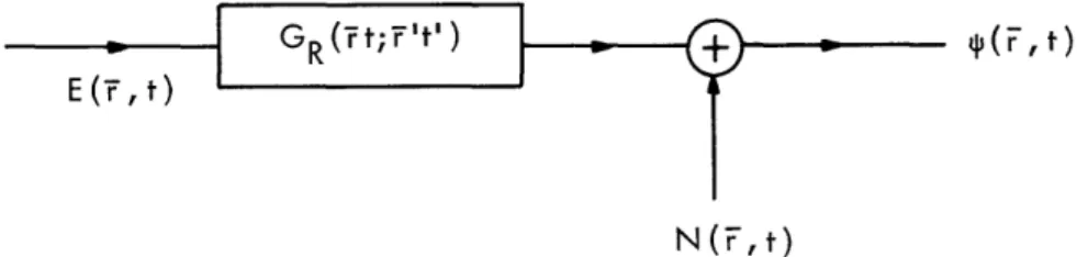
A nondifferential distributive description like the one discussed in section 2. 2 can be represented in the form of Fig. 2, wherein GR(rt;r't') can also be random.

E ( , t)

N (, t)

Fig. 2. Randomly time-variant nondifferential linear distributive channel.

This case can still be considered a special case of the following differential system representation if GR(rt; r't') can be interpreted as the stochastic Green's function of a random differential equation. In this case we have Fig. 3.

E (Fr, t)

N(Fr, t)

Fig. 3. Randomly time-variant differential linear distributive channel.

25

_111111111__11__1_11_··I----·---··I-In the previous discussions we have only treated the output 4(F, t). A specified addi-tive noise field N(r,t) can evidently be introduced with a combined representation

1'(r, t) = f fV GR(rt; r't')[E(r',t')+ (r,t')] dr'dt' + N(r,t). (91)

The initial conditions have been suppressed as explained previously. It is simple to give the representation of Fig. 1,

P(t) = f h(t, -) S(T) d + n(t), (92)

from the distributive representation (91) when we know that

P(t)= fV q'(Ft) u() d. (93)

u

Such a relation is indeed what usually occurs, say, when we look at a coherence area on the received plane of an optical channel. If in this case the signal s(t) is generated by a point source at r = 0 E(r,t) = 6(t) 6(r), we have h(t,) = fto fV G(Ft;F't') u() dFrdt' u n(t) = ft f Vf dtdrdr' G(t; r't') u(F) F(r',t') + fV u(F) N(r, t) dr. 2 u u

It is obvious that it is not generally possible to obtain (91) from the representation (92) even if we know that (t) is obtained through (r,t) with a given u(r), as in (93). This should not bother us, since only the representation (91) is a complete specification of the situation under consideration. We shall always regard the classical specification to be given only if each function or process on the right side of (91) is specified. We require such complete specification even when we are ultimately interested only in (92). This is because physical aspects need to be explicitly invoked in the quantum treatment; for example, the nature of the variable p(t) is involved.

When a complete specification is given in the form (91) it is clear that we can form still more general communication systems than the one shown in Fig. 1. If we let

ak = f '(F, t) ak(F, t) drdt'

for ordinary functions { k(F, t)}, we can determine the joint distribution of {ak, ak} in

26

a straightforward fashion. When

Sk(r,t) = u(r) 6(t-t') (94)

we would recover the system (92), in that a = (t). In general, a choice of {ak} reflects to a certain extent the physical receiver structure or configuration.

2. 7 Conclusion

We have developed the theory of classical random field propagation in a particular form convenient for translation to quantum treatment. A description of classical com-munication systems from this framework has also been given. The novel feature in our discussion is that the differential equation channel characterization is quite physical, in that it describes the field transmission in the system of interest and is related rather intimately to a fundamental Hamiltonian treatment. These points will be discussed fur-ther in the quantum case.

Another apparently new concept that we have introduced is the notion of a random Green's function which is particularly important when we use a differential equation phys-ical description. When available, it provides complete information on the solutions of a stochastic differential equation. It should be worthwhile to investigate such functions further because they would have applications in many other areas.

Finally, we would like to mention that the description of communication systems by differential equations, together with appropriate physical interpretations, should provide a useful approach to general communication analysis.

27

C. QUANTUM RANDOM PROCESSES

We shall now develop an operational theory of quantum random processes to a degree sufficient for our future purposes. We shall use the fundamental results established here to obtain quantum-channel representations. Rigorous mathematical discussions of

ordinary stochastic processes may be found in many places.9 1 9 4 General mathematical formulations of quantum dynamical theory, with due regard to the statistical nature peculiar to quantum mechanics, also exist in a variety of forms.5'8'1 1 1 - 1 2 2 The most common form is briefly reviewed in Appendix A. There does not exist, to the author's knowledge, any systematic and convenient mathematical theory of random processes applicable to situations in quantum physics, although there are fragmentary works both

of a mathematical 1 1 6, 117 and of a calculational nature.69-73 In addition, some proba-bilistic notions and techniques related to quantum statistical dynamical problems have been used by physicists. 9 73, 118 In spite of this, it is highly desirable, at least for applications to communication and other systems, to have a common framework for treating quantum random problems that is comparable in scope to the discussion of classical stochastic problems by ordinary random processes. It is our purpose to

sketch a primitive version of such a novel theory.

By a quantum random process we mean a time-dependent linear operator X(t), which is defined on the state space of the quantum system under consideration and possesses a complete set of eigenstates for every t. A quantum random process, which we often abbreviate as a quantum process, is therefore a quantum observable in the Heisenberg

(or H) picture. See Appendix A for more detailed discussion. We shall first discuss time-independent operators and then we treat the time-dependent case.

It is appropriate to emphasize, first, the differences between our present treatment and that of ordinary stochastic processes. In the classical case the system under con-sideration, composed of functions f(X) of a random variable X, is completely character-ized by the distribution function of X alone. In quantum theory we cannot obtain the dis-tribution of an f(X) from that of X in the classical manner when X is non-Hermitian.

Complete statistical characterization of a quantum system is given differently, usually through a density operator. The purpose of our development is to establish convenient statistical specifications of a quantum system, while maintaining, as much as possible, the applicability and usefulness of ordinary stochastic concepts and methods. Similarly to the classical case, such concepts and methods make possible the efficient analysis of many quantum statistical problems.

3. 1 Quantum Probabilistic Theory

We have to develop some probabilistic concepts applicable to the quantum case before we can start our discussion of quantum processes. Appendix A gives a brief introduc-tion to quantum formalism and to some of the definiintroduc-tions that we use. The essential point of our treatment is to give a c-number description of the quantum observables

28