HAL Id: tel-01133165
https://tel.archives-ouvertes.fr/tel-01133165
Submitted on 18 Mar 2015HAL is a multi-disciplinary open access archive for the deposit and dissemination of sci-entific research documents, whether they are pub-lished or not. The documents may come from teaching and research institutions in France or abroad, or from public or private research centers.
L’archive ouverte pluridisciplinaire HAL, est destinée au dépôt et à la diffusion de documents scientifiques de niveau recherche, publiés ou non, émanant des établissements d’enseignement et de recherche français ou étrangers, des laboratoires publics ou privés.
the human hippocampus in large populations.
Claire Cury
To cite this version:
Claire Cury. Statistical shape analysis of the anatomical variability of the human hippocampus in large populations.. Neurons and Cognition [q-bio.NC]. Université Pierre et Marie Curie - Paris VI, 2015. English. �NNT : 2015PA066021�. �tel-01133165�
Sp´ecialit´e Neurosciences ´
Ecole Doctorale Cerveau, Cognition, Comportement (ED3C)
Pr´esent´ee par
Claire CURY
Analyse statistique de la variabilit´
e anatomique de
l’hippocampe `
a partir de grandes populations.
soutenue le 12 F´evrier 2015
Membres du jury
Dr. Arnaud Cachia Rapporteur
Dr. Olivier Coulon Rapporteur
Dr. Habib Benali Examinateur
Dr. Jean-Fran¸cois Mangin Examinateur
Dr. Roberto Toro Membre invit´e
Dr. Joan Alexis Glaun`es Co-encadrant Dr. Olivier Colliot Directeur de th`ese
Contents 3
Résumé français 1
1 Introduction 13
I Background
21
2 The human hippocampus 23
2.1 Anatomy, development and variability . . . 24
2.1.1 Terminology . . . 24
2.1.2 Spatial localisation . . . 25
2.1.3 Anatomy. . . 27
2.1.4 Development . . . 30
2.1.5 Incomplete hippocampal inversion . . . 35
2.2 Visualisation in MRI . . . 38 2.3 Role . . . 41 2.3.1 Memory . . . 42 2.3.2 Spatial navigation. . . 45 2.3.3 Pathologies . . . 46 2.4 Conclusion . . . 50 3 Computational anatomy 51 3.1 Shapes and their numerical representation in medical imaging . . . . 53
3.1.1 Data acquisition. . . 53
3.1.2 Segmentation . . . 54
3.2 Shape descriptors and dissimilarity . . . 55
3.2.1 Common shape descriptors . . . 56
3.2.2 Deformation-based descriptors . . . 59
3.3 Chosen mathematical model . . . 61
3.3.1 Currents . . . 62
3.3.2 LDDMM framework . . . 67
3.3.2.1 Large Diffeomorphic Deformations. . . 67
3.3.2.2 Geodesic equations and local encoding. . . 70
3.4 Statistical shape analysis . . . 71
3.4.1 Geometry based methods. . . 72
3.4.1.1 Distance matrix approximation . . . 72
3.4.2 Principal component analysis on initial momentum vectors . . 74
3.5 Template estimation . . . 75
3.6 Conclusion . . . 78
II Contributions
81
4 Evaluation of Incomplete Hippocampal Inversions 83 4.1 Introduction . . . 844.1.1 Review of the Incomplete Hippocampal Inversion . . . 86
4.1.2 Criteria used in the literature . . . 89
4.2 Participants and MRI data . . . 92
4.3 Simplified individual criteria and global criterion for IHI assesment . 93 4.3.1 Criterion C1: verticality and roundness of the hippocampus body . . . 93
4.3.1.1 Description . . . 93
4.3.1.2 Examples . . . 95
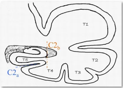
4.3.2 Criterion C2: collateral sulcus . . . 97
4.3.2.1 Description . . . 97
4.3.2.2 Examples . . . 100
4.3.3 Criterion C3: medial positioning . . . 101
4.3.3.1 Description . . . 101
4.3.3.2 Examples . . . 102
4.3.4 Criterion C4: subiculum . . . 103
4.3.4.1 Description . . . 103
4.3.5 Criterion C5: sulci of the fusiform gyrus (T4) . . . 104 4.3.5.1 Description . . . 104 4.3.5.2 Examples . . . 105 4.3.6 Global criterion C0 . . . 105 4.4 Hippocampus segmentation . . . 106 4.5 Experiments . . . 107 4.5.1 Java application . . . 107 4.5.2 IHI assesment . . . 109
4.5.3 Intra- and inter-observer reproducibility . . . 109
4.5.4 Statistical analysis . . . 110
4.6 Results . . . 110
4.6.1 Intra- and inter-observer reproducibility . . . 110
4.6.2 Global criterion C0 . . . 111
4.6.3 Individual criteria . . . 113
4.6.4 Impact of IHI on the automatic segmentation . . . 115
4.7 Discussion and conclusion . . . 117
5 Diffeomorphic iterative centroid method for template estimation on large datasets 121 5.1 Introduction . . . 122
5.2 An Iterative Centroid method . . . 125
5.2.1 Mathematical justification . . . 126
5.2.2 Diffeomorphic Centroid methods . . . 128
5.2.2.1 Direct iterative centroid . . . 129
5.2.2.2 Centroid with averaging in the space of current . . . 130
5.2.2.3 A pairwise centroid . . . 131
5.2.3 Implementation . . . 132
5.3 Results . . . 135
5.3.1 Data . . . 135
5.3.2 Effect of subject ordering. . . 137
5.3.3 Position of the centroids within the population . . . 141
5.3.4 Effects of initialization on estimated variational template . . . 142
5.3.5 Effect of the number of iterations for Iterative Centroids . . . 145
5.3.6 Computation time . . . 146
5.4 Discussion . . . 147
6 Statistical shape analysis using diffeomorphic iterative centroids 151 6.1 Introduction . . . 152
6.2.1 Statistical Analysis . . . 153
6.2.1.1 Principal Component Analysis on initial momentum vectors. . . 153
6.2.1.2 Distance matrix approximation . . . 154
6.2.2 Data . . . 155
6.2.3 Experiments . . . 157
6.2.4 Synthetic dataset SD . . . 158
6.2.4.1 Computation time . . . 158
6.2.4.2 Centring of the centres . . . 159
6.2.4.3 PCA . . . 161
6.2.4.4 Distance matrices . . . 161
6.2.5 The real dataset RD50 . . . 164
6.2.5.1 Computation time . . . 165
6.2.5.2 Centring of the centres . . . 165
6.2.5.3 PCA . . . 167
6.2.5.4 Distance matrices . . . 170
6.3 Variability analysis and prediction of IHI . . . 173
6.3.1 Centroid estimation . . . 173
6.3.2 Prediction of IHI using shape analysis. . . 176
6.4 Discussion and conclusion . . . 180
7 Shape analysis applied to the Alzheimer’s disease 183 7.1 Dataset and experiments . . . 184
7.2 Results: analysis of variability . . . 185
7.3 Results: prediction of clinical variables . . . 189
7.4 Conclusion . . . 192
8 Conclusion and discussion 195
List of Figures 200
List of Tables 207
introduction L’analyse statistique de la forme des structures anatomiques est un enjeu essentiel pour de nombreuses applications : modélisation de la variabilité normale et pathologique, prédiction de paramètres cliniques et biologiques à partir de données anatomiques. Ces dernières années ont vu l’émergence de grandes bases de données en neuroimagerie, offrant une puissance statistique considérablement accrue.
Cette thèse a pour thème l’étude statistique de la variabilité anatomique de l’hip-pocampe à partir de grandes bases de données. Après un état de l’art, la première partie de la thèse porte sur l’étude d’une variante anatomique appelée inversion in-complète de l’hippocampe (IHI). Pour ce faire, nous avons mis au point une échelle de cotation des inversions incomplètes de l’hippocampe (IHI). Elle a été ensuite ap-pliquée à 2000 sujets sains jeunes de la base données multicentrique IMAGEN. C’est la première fois que ces variants anatomiques sont étudiés sur une grande population de sujets sains.
La seconde partie de la thèse porte sur la mise au point d’une méthode d’analyse statistique de formes utilisant les grandes déformations difféomorphiques et les cou-rants mathématiques, qui soit utilisable pour l’analyse de grandes bases de données. Nous avons en particulier introduit une nouvelle approche rapide pour construire des prototypes anatomiques. Cette approche a été validée sur 1000 sujets sains jeunes de la base de données IMAGEN et environ 300 sujets (sujets sains âgés et patients atteints de maladie d’Alzheimer) de la base de données ADNI.
Chapitre 2 : présentation de l’hippocampe L’hippocampe est une structure du cerveau bilatérale située dans le lobe temporal, dont la forme a d’abord évoqué une virgule avant d’être comparée à un hippocampe en 1587 par un anatomiste italien (G C Aranzio). La tête (la partie renflée) est suivie d’un corps allongé (le corps) et d’une extrémité dentée (la queue). Il est composé de 2 lames de cortex enroulées l’une sur l’autre, la Corne d’Ammon et le Gyrus Denté, séparés par le sillon hippocampique. L’hippocampe appartient au système limbique, véritable interface entre le tronc cérébral et le neocortex. Les informations neuronales circulent entre le cortex entorhinal et le neocortex et vice versa (circuit de Papez) et sont impliquées dans les processus de mémorisation.
Lors du développement embryonnaire, l’hippocampe commence à être différencié aux alentours de la 10ème semaine d’aménorrhée (SA) pour certains. A 30 SA l’hip-pocampe est pratiquement comme chez l’adulte. Pendant la gestation, l’hipl’hip-pocampe va s’inverser c’est à dire que la corne d’Ammon et le gyrus denté vont s’enrouler l’un autour de l’autre, pour former comme deux "U" emboîtés. Cette inversion n’est en réalité pas toujours complète, ce qui amène à un variant anatomique appelé inversion
incomplète de l’hippocampe. Ce variant anatomique à été fréquemment observé chez des patients épileptiques mais aussi chez des sujets non épileptiques. Cette inversion incomplète est retrouvée plus généralement chez les hippocampes gauches.
Les techniques d’imagerie par résonnance magnétique (IRM) permettent de consti-tuer de grandes bases de données et d’observer l’hippocampe in vivo grâce notam-ment à des séquences 3D pondérées en T1.
La fonction de l’hippocampe est essentielle dans les mécanismes de la mémoire et pour la localisation spatiale. Des études sur des patients ayant subit une ablation des hippocampes ont montré que l’hippocampe serait alors impliqué dans la création de nouveaux souvenirs et dans la mémoire épisodique.
On retrouve l’hippocampe impliqué dans des pathologies comme la maladie d’Alzheimer dont il est l’une des premières structures à être atteinte par atrophie ; l’épilepsie dont il peut être le foyer des crises dans le cas des épilepsies du lobe temporal ; et la dépression pour laquelle son volume serait un facteur de risque tout comme pour les patients atteints de schizophrénie.
Chapitre 3 : l’anatomie numérique Une fois la forme globale de l’hippocampe décrite, nous allons nous intéresser a la variabilité de sa forme, afin de pouvoir dif-férencier les formes correspondant à un sujet normal de celles correspondant à une pathologie ou de pouvoir étudier les variations anatomiques de la structure étudiée. Il faut avant tout définir ce qu’est une forme. En effet ce terme est assez mal défini et pour analyser la forme nous avons besoin d’un descripteur de forme et d’une mesure de dissimilarité qui dans certains cas découle du descripteur ; il faut trouver un équi-libre entre la capacité du descripteur à garder l’information de la forme et une mesure
de dissimilarité proche d’une vraie distance invariante par transformations rigides. Ici une forme est le contour d’un objet 2D ou 3D représenté par un masque binaire ou par des points 2D ou 3D. Pour obtenir notre forme, il faut isoler la structure de l’hippocampe du reste du cerveau, par segmentation pour ainsi obtenir un masque binaire 3D que l’on convertit en maillage 3D. Il faut ensuite choisir un descripteur permettant de décrire la forme. Plusieurs choix de modèle sont possibles, et nous avons choisi de travailler dans le cadre des grandes deformations diffeomorphiques (LDDMM), deja utilisées dans de nombreux travaux de recherche pour l’étude de la variabilité des structures cérébrales car les déformations sont des difféomorphismes qui permettent de prendre en compte des formes assez différentes tout en respec-tant l’organisation de la structure et en caprespec-tant des variations locales non linéaires. L’inconvénient d’utiliser de telles déformations est que la phase d’optimisation est très coûteuse en terme de temps de calcul. Pour représenter nos formes d’hippo-campe nous avons choisi d’utiliser les « courants », objet mathématique qui sert à modéliser des objets géométriques sans correspondance point à point. Les formes ainsi décrites ont l’avantage de se trouver dans un espace vectoriel, qui permet alors d’additioner ou soustraire des formes entre elles. Glaunès et al. ont introduit cet objet mathématique pour l’analyse anatomique numérique en 2005.
La combinaison des LDDMM et des "courants" nous permet alors de construire un modèle de la population. Généralement les formes sont analysées par leurs défor-mations depuis le modèle de la population. Pour l’analyse statistique de ces formes nous utilisons une ACP sur les vecteurs moments initiaux venant du modèle et allant vers les formes. Ces vecteurs moments initiaux on l’avantage de déterminer
entiè-rement la déformation de la forme, tel un vecteur vitesse initial lors d’un lancer de projectile.
Pour ce qui est du calcul du modèle de la population (la partie la plus imposante du processus d’analyse de la forme basée sur un modèle en terme de temps de calcul), il y a plusieurs méthodes proposées dans la littérature qui sont toutes coûteuses en temps de calcul, ce qui est un frein à l’analyse de grandes bases de données. Nous allons nous intéresser à une méthode qui n’admet aucun a priori sur la forme du modèle. De cette méthode va découler la méthode que nous allons présenter au chapitre 5 puis utiliser dans les analyses de cette thèse.
Chapitre 4 : Étude des inversions incomplètes de l’hippocampe Dans ce chapitre nous présentons les critères utilisés pour l’évaluation des Inversions Hip-pocampique Incomplètes (IHI). La fréquence des IHI dans la population saine est mal connue. On sait seulement que ce variant anatomique de l’hippocampe semble plus présent chez les sujets épileptiques et qu’il est présent chez les sujets sains, mais cette fréquence varie beaucoup suivant les critères utilisés pour déterminer si l’hippocampe présente une IHI et suivant la population utilisée. Nous allons donc étudier les IHI sur une grande base de données (pour une bonne puissance statis-tique) composée de 2008 sujets, et nous allons faire en sorte d’avoir des critères simples et reproductibles. Dans la littérature beaucoup de critères ont été utilisés, souvent de manière très subjective, pour décrire les IHI. Nous avons choisis d’uti-liser les critères les plus récurrents qui semblent aussi les plus faciles à caractériser afin d’en faire des critères reproductibles pour l’évaluation d’une grande base de données. Les critères retenus sont : le critère C1, qui porte sur la rondeur et la
ver-ticalisation de l’hippocampe dans les coupes coronales du corps, le critère C2 qui porte sur la profondeur du sillon collatéral et son orientation, le critère C3 qui porte sur la position plus ou moins médiale de l’hippocampe, le critère C4 qui porte sur un potentiel épaississement anormal du subiculum, et finalement le critère C5 qui porte sur les deux sillons du gyrus fusiforme et qui indique si l’un de ces sillons dépassent latéralement l’hippocampe au niveau du subiculum. Un critère global C0 a aussi été utilisé ; il note l’aspect général de l’hippocampe et indique si il présente une IHI ou non. Ces critères ont été notés sur 2008 sujets de la base européenne IMAGEN composée de jeunes (entre 13 et 15 ans) sujets sains. Les notes ont été données par 2 observateurs CC et FC, ainsi que la qualité des segmentations des hippocampes faites par le logiciel de segmentation automatique SACHA. 42 sujets ont été utilisés pour tester la reproductibilité inter et intra observateurs des critères de IHI. Un kappa test nous permet de dire que ces critères, comme détaillé dans ce chapitre, sont reproductibles (kappa > 0.64 pour tous les critères). Dans ce chapitre on remarque aussi que les segmentations sont corrélées aux IHI : plus l’hippocampe présente une IHI, moins sa segmentation est fiable. Cependant certains hippocampes présentant des IHI ont tout de même eu une segmentation correcte. Le critère global C0 donne une prévalence de 17% de IHI à gauche et de 6.5% à droite avec de chaque coté des intervalles de confiance assez petits. On a aussi observé qu’il n’y avait pas de différences entre hommes et femmes, ni entre droitiers et gauchers. L’analyse des critères individuels nous indique que les répartitions des notes de chacun de ces cri-tères sont différentes entre le côté droit et le côté gauche ; les notes sont généralement plus élevées à gauche qu’à droite. La somme des 5 critères individuels (IHI score),
montre qu’il y a une sorte de continuum entre les notes ; il n’y a pas de de coupure évidente. Cette somme de critères peut être utilisés comme un indicateur du degrés de l’IHI. Cependant en catégorisant par le critère global, on a remarqué que les hippocampes sans IHI se séparent plutôt correctement bien des hippocampes avec IHI. Un seuil à donc été calculé pour déterminer à partir de quel score l’hippocampe semble avoir probablement une IHI, afin de pouvoir faire des études de groupes en utilisant uniquement les critères individuels présentés ici.
Chapitre 5 : Barycentre difféomorphique itéré Dans ce chapitre nous pré-sentons la méthode des barycentres itérés basée sur la théorie des déformations difféomorphiques. Comme énoncé dans les chapitre 3, le modèle de forme utilise une représentation en tant que courants mathématiques. L’idée de la méthode est d’améliorer l’initialisation de la méthode présentée par Glaunès et al. (2006) en four-nissant à la méthode une meilleure initialisation, plus proche du résultat final. L’idée de cette méthode est de calculer un barycentre itératif dans l’espace des déforma-tions. Le barycentre est initialement choisi comme l’un des sujets de la population, puis on effectue un recalage de ce sujet vers un autre sujet et on stoppe la défor-mation au milieu de la trajectoire pour ainsi obtenir le barycentre de 2 sujets. On ajoute d’autres sujets au barycentre en itérant le processus : on recale le barycentre actuel vers un troisième sujet et on stoppe la déformation à 1/3 de la trajectoire de déformation pour obtenir le barycentre de 3 sujets. Le barycentre ainsi calculé dans un espace euclidien, est le centre exact de la population, et son calcul ne dé-pend pas de l’ordre des sujets. Mais ici nous utilisons des recalages inexacts (du fait des maillages différents, et de la différence trop importante entre certaines formes)
dans des espaces courbes, ce qui ne permet pas d’atteindre le centre exact et rend le calcul du barycentre dépendant de l’ordre des sujets. Nous proposons 3 algorithmes différents pour la mise à jour du barycentre. Pour connaître l’impact de l’ordre des sujets sur le centrage du barycentre nous avons fait des expériences sur trois bases de données. Data1 est composé de 500 maillages simples (135 sommets) d’hippocampes formés à partir d’un maillage d’hippocampe et de déformations principalement dif-féomorphiques, Data2 est composé de 95 hippocampes avec les mêmes maillages (1001 sommets), et RealData est composé des mêmes 95 hippocampes que Data2, avec des maillages différents pour chaque hippocampe. 10 ordres différents ont été utilisés pour générer 10 barycentres différents pour chaque dataset. Les distances entre les différents barycentres sont petites comparées aux distances de la popula-tion. Visuellement ces différences sont à peine visibles. On a évalué le centrage des barycentres en utilisant le ratio entre la norme des vecteurs moments initiaux et la moyenne des normes des vecteurs moments initiaux. Le centrage est meilleur pour le dataset Data1 que pour les deux autres datasets car il comporte des maillages plus simples. Le centrage pour Data2 est similaire au centrage pour RealData, ce qui nous permet de dire que la différence de maillages utilisés à très peu d’influence sur le résultat final. On a aussi observé que ces barycentres utilisés comme initialisa-tion d’une méthode variainitialisa-tionnelle d’estimainitialisa-tion de template permettent un meilleur résultat final. Cependant le temps de calcul de la méthode du barycentre itéré est beaucoup plus petit que celui de la méthode variationnelle d’estimation de template ; de plus la méthode des barycentres fournit déjà un assez bon résultat de centrage, ce qui permet d’envisager d’utiliser un barycentre directement comme un template de
la population, pour par la suite analyser cette population par rapport à ce template. Chapitre 6 : analyse de formes statistique basée sur le barycentre itéré Dans ce chapitre nous utilisons le barycentre itéré d’une population comme template pour l’analyse de la variabilité anatomique par analyse en composantes principales (ACP) sur les vecteurs moments initiaux ou les matrice de distances approximées. On utilise ici 3 datasets, le premier est un dataset synthétique (SD50) calculé à partir d’un maillage d’hippocampe. Les 50 formes de ce dataset sont construites en utilisant des déformations difféomorphiques, de sorte que le maillage d’hippo-campe initial se trouve exactement au centre de la population, et que le centre de cette population est connu. Le dataset RD50 est un sous ensemble de 50 maillages d’hippocampes de la base IMAGEN, et le dataset RD1000 est un sous ensemble de 1000 maillages d’hippocampes de la base IMAGEN. Des expériences ont été faites sur les datasets SD50 et RD50. Nous avons testé le centrage des barycentres de ces populations à l’aide du ratio décrit dans le paragraphe précédent. Pour SD les barycentres, ainsi que les templates variationnels calculés à partir de la méthode de Glaunès et al. sont très proches du vrai centre de cette population, mais aucun n’est à sa position exacte. Pour RD50, les ratios de centrage des templates (barycentre et template variationnels) sont évidemment moins bons, mais sont tous du même ordre et semblent proche les uns des autres par rapport au reste de la population. Ils sont tous plus proches du centre que n’importe quel sujet du dataset. Pour le dataset SD50, les résultats de l’ACP sur les vecteurs moments initiaux depuis les barycentres sont très similaires au résultat de l’ACP obtenu à partir du vrai centre du dataset. Pour RD50, les courbes de variance expliquée cumulative sont très
si-milaires entre celles calculées à partir des barycentres et celles calculées à partir des templates variationnels. De même pour les matrices de distances approximées, elle sont également différentes de la matrice de distances directes (calculée en déformant les sujets 2 à 2). l’analyse de formes en utilisant les barycentres donne des résultats similaires, de plus le calcul du barycentre est beaucoup plus rapide que le template variationnel. Pour appliquer ce pipeline, on applique ce calcul de barycentre sur le dataset RD1000 issu de IMAGEN, dont les sujets ont tous reçu un IHI score (voir chapitre 4). On a pu remarquer que le barycentre était plutôt bien centré dans la po-pulation, et que l’ACP pouvait expliquer plus de 97% de la variabilité anatomique de cette population à l’aide de 50 dimensions. Il est intéressant de noter que ce nombre de dimensions est stable quand on inclut un nombre de sujets suffisamment élevé. Nous avons par la suite utilisé quarante dimensions de l’ACP pour essayer de prédire les scores IHI à l’aide d’une régression linéaire multiple. On a réussi en uti-lisant entre 20 et 40 dimensions à prédire les score IHI avec une corrélation de 69%. Les modales de régression linéaire ont été validées par une méthode de validation croisée k-fold avec k=100.
Chapitre 7 : analyse de formes appliquée à des patients Alzheimer Dans ce chapitre nous appliquons la méthode rapide d’analyse de forme utilisant un ba-rycentre à des hippocampes de la base ADNI composée de sujets âgés sains (groupe CN) et de sujet atteints de la maladie d’Alzheimer (groupe AD). La population est composée de 160 CN et de 134 AD. Tous ces sujets ont un score MMSE (Mini Mental State Examination) indicateur global de démence et un score ADNI-MEM qui est un score composite reflétant les performances des sujets à des tests de
mé-moire. Dans un premier temps nous comparons le barycentre du groupe CN à celui du groupe AD, et nous constatons que le premier axe de variation est très différent entre ces deux groupes. De plus le groupe AD a besoin de moins de dimensions pour expliquer sa variance anatomique (environ 60 contre 80 pour le groupe CN). A l’aide du barycentre de la population totale, nous projetons ensuite le premier axe de chaque groupe sur les 2 premiers axes des groupes, ce qui nous permet de voir que ces 2 groupes se différencient déjà sur les 2 premières dimensions de l’espace ACP de la population totale. Nous nous sommes ensuite intéressés à la prédiction des notes MMSE et ADNI-MEM dans la sous population des sujets âges sains en utilisant les 50 premières dimensions de l’espace ACP. Nous observons alors que comme prévu la prédiction du résultat du test MMSE est mauvaise et la prédiction de ADNI-MEM score est assez bonne ; une trentaine de dimensions suffisent à pré-dire le score ADNI-MEM. Le resultat est logique, car le ADNI-MEM score reflète les performances de mémoire pour lesquelles l’hippocampe joue un rôle central, alors que le score MMSE est un indicateur global de la démence. Il serait donc bien éton-nant que l’hippocampe seul arrive à prédire un tel indicateur. On en conclut donc que notre méthode d’analyse de forme produit des résultats cohérents.
conclusion Pour ce travail de thèse qui consistait à analyser la variabilité anato-mique de l’hippocampe sur de grandes bases de données, nous avons d’une part mis au point une méthode d’analyse de forme de l’hippocampe applicable à de grandes populations. D’autre part, nous avons étudié une forme anatomique particulière de l’hippocampe, l’IHI qui pourrait être d’origine développementale et qui a été sur-tout étudiée dans des populations épileptiques. Nous avons mis au point des critères
robustes d’évaluation des IHI, qui permettront par la suite de comparer les études. On a pu remarquer dans ce travail que les IHI ne sont pas rare puisque présentent dans environ 20% de la population. L’analyse de forme utilisant un template de la population que nous avons mise au point est capable de capturer la variabilité ana-tomique des hippocampes avec peu de variables et est capable de prédire certains paramètres biologiques comme la présence ou non d’IHI ou certain paramètres cli-niques comme le score ADNI-MEM chez les sujets âgés sains. Il reste des questions auxquelles il serait intéressant de trouver une réponse. Premièrement, est ce que les IHI sont des variants anatomique qui affectent uniquement l’hippocampe ou non. Il serait intéressant de s’intéresser aux relations entre IHI et les sillons adjacents. D’autres parts, les facteurs génétiques et/ou environnementaux du développement de ces IHI sont encore inconnus. D’un point de vue méthodologique, il y a aussi plusieurs perspectives. Il serait intéressant de comparer la méthode des barycentres à d’autres méthodes de création de template. Il serait aussi intéressant de regarder l’impact du calcul de barycentre sur une population constituée de structures plus complexes comme les sillons par exemples.
Introduction
The hippocampus is a brain structure involved in important cognitive functions as memory processes, long term memorisation and in spatial navigation. Another fascinating feature of the hippocampus is that it preserves its ability to generate neurons throughout life (Eriksson et al., 1998) by dividing progenitor cells in the dentatus gyrus, one of the two cortical lamina composing the hippocampus. Studies found that hippocampi are involved in many pathologies and psychiatric disorders such as Alzheimer’s disease, epilepsy, depression and schizophrenia.
The anatomy of the human brain is highly variable. The genetic and envi-ronmental bases of this variability remain largely unclear. So does the influence of anatomical variability on the development of pathologies or cognitive functions. The anatomy of the hippocampus is also variable. A particularly remarkable anatomical variant of the hippocampus is the Incomplete Hippocampal Inversion (IHI). Indeed an inversion of the hippocampus occurs around the 25 gestational week. When the inversion is not completed, this results in the anatomical variant named IHI. This Incomplete Hippocampal Inversion is characterized by shape changes visible on Magnetic Resonance Images. IHI have been mostly described in patients with epilepsy, in which they are highly frequent (Baulac et al., 1998). However, they are also present in healthy subjects although their prevalence and characteristics have not been rigorously studied.
Magnetic Resonance Images (MRI) allows exploring brain anatomy in vivo. The generalization of MRI has made it possible to study anatomical variability in large populations. This allows studying statistically normal and abnormal developmental patterns and their correlation with cognitive, behavioural, genetic or environmental variables.
The objective of Computational Anatomy (CA) is to mathematically model and analyse the anatomical variability of biological structures. The study of biological shape variability has been first introduced by the famous biologist but also mathe-matician D’Arcy Thompson (D’Arcy Thompson, 1917). Since that time significant efforts have been made to develop a theory for statistical shape analysis. In the past years, a large number of statistical shape analysis methods have been proposed to
quantitatively analyse the variability of biological shapes. Among these, an interest-ing framework for anatomical shape analysis is the Large Diffeomorphic Deformation Metric Mapping (LDDMM) framework that quantifies differences between shapes via smooth deformations which capture the global and local non-linear variations while preserving the anatomical structure organisation. Another attracting feature of the LDDMM framework is that deformations are entirely parametrised by vectors lying in vector space, providing a natural setting for statistical analysis. Moreover, the framework of currents can be used to represent the shapes without assuming point-to-point correspondence accross subjects. A now classical method is to com-pare shapes to a template of the population, this is named template-based shape analysis. These last years we have seen the emergence in neuro-imaging of large databases. However, the application of LDDMM approaches to large datasets is difficult because of their high computational load. Faster approaches for LDDMM-based template estimation are then needed for the analysis of large databases.
∗ ∗ ∗
The goal of this thesis is to develop and evaluate methods to study the anatom-ical variability of the hippocampus using large databases. Our developments were made in the framework of LDDMM for modeling deformations, and of currents for modeling anatomical surfaces. Within these frameworks, we aimed to develop fast approaches for template-based shape analysis. Our goal was then to apply these approaches to predict the presence of specific anatomical variants as well as the variation of cognitive or clinical variables. In particular, we were interested in the
prediction of the presence of Incomplete Hippocampal Inversions (IHI). To that aim, we also needed to visually characterize the presence of this variant in a given population.
We first focused on the evaluation of the Incomplete Hippocampal Inversions (IHI). To this aim, we proposed a new set of criteria to evaluate IHI, by adapting criteria from the litterature. This new set of criteria is adapted to the evaluation of large datasets. These criteria were applied to study the prevalence and charac-teristics of IHI in a database of over 2000 MRI of young healthy subjects from the multi-centric European database IMAGEN. We also explored the impact of IHI on automatic hippocampal segmentation, the differences between males and females, and between right and left sides. This is the first time that this anatomical variant has been studied on a large dataset of healthy subjects.
Than, we developed and evaluated a new statistical shape analysis method adapted to the study of large databases. Its principle is that of template-based shape analysis, in which every indivual shape is characterized through its deforma-tion from a template of the populadeforma-tion. In particular, we proposed new approaches for fast estimation of population templates. They are based on the estimation of population centroid using iterative diffeomorphic matchings. The centroid can then be directly used as a template, or as an initialization for another template esti-mation method. We performed various experiments to evaluate the properties of the centroid, its robustness and its impact on statistical results. We then applied this method to a template-based statistical shape analysis on 1000 young healthy subjects of the IMAGEN database, in which we aimed to predict the IHI score
pre-viously evaluated. We also applied this method to a dataset composed of around 300 subjects of the Alzheimer’s Disease Neuroimaging Initiative (ADNI) database (Alzheimer’s disease patient and elderly controls), in which we aimed to predict the memory score in Alzheimer’s disease patients population.
∗ ∗ ∗
The rest of this manuscript contains the following chapters.
Chapter 2 In this chapter, we briefly review the anatomy, development and roles
of the hippocampus. We also quickly present Incomplete Hippocampal Inversions.
Chapter 3 This chapter first presents different ways to describe a shape and
different methods to analyse these shapes. We then present with more details the LDDMM framework and the use of currents for shape representation.
Chapter 4 This chapter presents a study of Incomplete Hippocampal Inversion
on a lare dataset of healthy subjects using visual criteria. We first present the criteria used in the literature to describe Incomplete Hippocampal Inversions, before introducing a new set of criteria. These are used for the evaluation of more than 2000 subjects of the database IMAGEN. We finally present results on the prevalence of IHI in the healthy population, the influence of the IHI on the quality control of segmentations, and results on the IHI score.
Chapter5 In this chapter, we present the diffeomorphic iterative centroid method
used to compute a centroid of the population. In this chapter the centroid is used to improve the initialization of a variational template estimation method.
Chapter 6 In this chapter, we use the diffeomorphic iterative centroid method
directly as a template of the population. We show that using the centroid as a template is sufficient for a template-based shape analysis of the hippocampus. We then use the result of the analysis to predict the IHI score.
Chapitre7 In this chapter, we apply the pipeline described in the previous
chap-ter to 298 subjects of the ADNI database (Alzheimer’s disease(AD) patients and elderly controls). We study anatomical differences between the two groups, and predict clinical parameters in the AD population.
Publications related to this thesis
Journal paper
Cury C., Glaunès J. A., Chupin M., Colliot O., and ADNI. (2015). Analy-sis of anatomical variability using diffeomorphic iterative centroid in patients with Alzheimer’s disease. Accepted for publication in Computer Methods in Biomechan-ics and Biomedical Engineering: Imaging and Visualisation.
Book chapter (peer-reviewed)
Cury, C., Glaunès, J. A., and Colliot, O. (2014). Diffeomorphic Iterative Cen-troid Methods for Template Estimation on Large Datasets. In F. Nielsen (Ed.), Geometric Theory of Information, Signals and Communication Technology (pp. 273–299). Springer International Publishing.
Conference papers (peer-reviewed)
Cury, C., Glaunès, J. A., Chupin, M. and Colliot, O., and ADNI. (2014). Fast Template-based Shape Analysis using Diffeomorphic Iterative Centroid. In C. C. Reyes-Aldasoro & G. Slabaugh (Eds.), MIUA 2014-Medical Image Understanding and Analysis 2014, (pp. 39-44), Egham, UK. (Best oral presentation award)
Cury, C., Glaunès, J. A., and Colliot, O. (2013). Template Estimation for Large Database: A Diffeomorphic Iterative Centroid method using Currents. In F. Nielsen & F. Barbaresco (Eds.), GSI2013 - Geometric Science of Information, volume 8085 of Lecture Notes in Computer Science (pp. 103-111).: Springer. Paris, France. (Oral presentation)
Conference abstract
Cury C., Glaunès J., Gerardin E., Chupin M. and Colliot O. (2012). Modelling morphological variability of the hippocampus using manifold learning and large de-formations. OHBM 2012 - 18th Annual Meeting of the Organization for Human Brain Mapping, Beijing, China. (Poster presentation)
Submitted journal paper
Cury C., Glaunès J. A., Toro R., Chupin M., Schumann G., Frouin V., Poline J.-B., and Colliot O. (2015). Statistical shape analysis of large datasets unsig Dif-feomorphic iterative centroids. Submitted to IEEE Journal of biomedical and health Informatics.
The human hippocampus
The hippocampus is a bilateral brain structure of the temporal lobe which is implicated in memory processes, spatial navigation and in some pathologies as Alzheimer’s disease, epilepsy depression or schizophrenia.
This chapter is organized as follows. In section2.1the description of the anatomi-cal structure of the hippocampal formation, his development, and a certain anatom-ical variation of the hippocampus are presented. In section 2.2 we describe how hippocampal anatomy can be studied in vivo using Magnetic Resonance Images.
We finally present the roles played by the hippocampus in memory processes, spa-tial navigation, and its implication in different neurological and psychiatric diseases in section 2.3.
2.1
Anatomy, development and variability
2.1.1
Terminology
Let’s start with a brief history of the origins of the term "hippocampus": this anatomical structure forms an arc with the anterior part larger than the posterior part, as a "comma". This identification as a comma did not become the reference, since in 1587 the anatomist Guilio Cesare Aranzio compared this structure to a "sea horse" (hippocampus in latin) or a "silkworm": the larger part corresponding to the head of the hippocampus and the narrower to the tail. Georges Duvernoy, in 1729, also compared this structure to a hippocampus or a silkworm. The physician J.B. Winslow in 1732 suggested the term "ram's horn". Then the surgeon R-J C de Garengeot used the term cornu Ammonis in reference to the egyptian god Ammon Kneph represented with ram's horn and lion's tail. Today it is the term "hippocam-pus" which refers to this cerebral structure located on the temporal lobe protruding in the lateral ventricles. The term cornu Ammonis is still used to describe one of the two cortical U-shaped lamina rolled up one inside the other which compose the hippocampus with the gyrus dentatus. In general the term "hippocampus proper" refers to the cornu Ammonis, the term "hippocampus" refers to the hippocampus proper plus the gyrus dentatus and the alveus (see section2.1), and the term
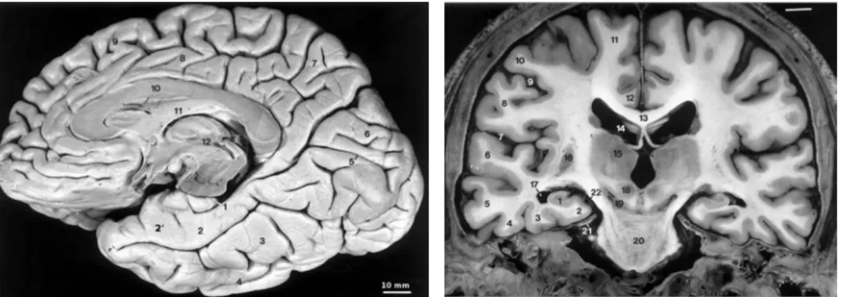
"hip-(a) 1 - hippocampus, 2 - parahippocampal gyrus (T5), 2´- enthorinal cortex, 3 - fusiform gyrus (T4), 4 infero temporal gyrus (T3), 5 -calcarine sulcus, 6 - occipital lobe, 7 - medial part of the parietal lobe, 8 - cingulate gyrus, 9 - medial part of the frontal lobe, 10 - corpus callosum, 11 - fornix, 12 - third ventricle
(b) 1 - hippocampus, 2 - parahippocam-pal gyrus (T5), 3 - fusiform gyrus (T4), 4 - infero temporal gyrus (T3), 5 - middle temporal gyrus (T2), 6 - superior tem-poral gyrus, 7 - lateral fissure, 12 - cingulate gyrus, 13 corpus callosum, 14 -lateral ventricle, 15 - thalamus, 18 - red nucleus, 20 - pons, 22 - ambient cistern
Figure 2.1: Dissection of the inferomedial part of the right hemisphere (a), and coronal section of a brain (b). FromDuvernoy (2005).
pocampal formation" includes the hippocampus and the subiculum.
2.1.2
Spatial localisation
The brain is composed of two hemispheres and each hemisphere is composed by different lobes:
– the frontal lobe located just behind the forehead is implicated in planning, voluntary movements and language
– the parietal lobe located to the rear is a sort of associative cortex of the sensory system and integrates information coming from vision, touch or hearing.
Figure 2.2: The limbic system
– the occipital lobe situated at the occipital bone is the center of the vision. – the temporal lobe situated behind each ear is related to multiple cognitive
processes such as language recognition and visual memory. It is divided in five convolutions.
The human hippocampus is a bilateral cerebral structure located in these temporal lobes, in the fifth convolution (T5) which has an internal positioning. Figure 2.1(b) shows the medial positioning of the hippocampus. The hippocampi form the medial and the bottom borders of the lateral ventricles. Figure2.1(a) shows that they have a longitudinal shape in a sagittal view. The anterior part of T5 is composed of the entorhinal cortex, directly connected to the anterior part of the hippocampus.
The hippocampus is also part of the limbic system, a "brain into the brain" (see Figure 2.2) described and discussed by Broca in 1877, Papez in 1937, Mac Lean in 1952 and Nauta in 1972. The limbic system corresponds to the deep and internal
Figure 2.3: Anatomy of the hippocampus. Left: general shape of the gyrus dentatus in an axial point of view. Right: the two cortical U-shaped lamina of the gyrus den-tatus (GD on the figure) and the cornu Ammonis (CA). A: head, B: body, C: tail, and right: the general shape of the hippocampus. Drawings are from Du-vernoy(2005)
regions of each hemisphere, such as T5 and the cingulate gyrus. It is composed of many structures (nuclei and primitive cortical areas) implicated in the memorisation process and emotions. The limbic system is the interface between the very "old" (from an evolutionary point of view) brain, the brainstem, and the very recent brain, the neocortex.
2.1.3
Anatomy
The hippocampus has an elongated shape in the rostro-codal direction as shown in Figure2.3with a length of 4 to 4.5 cm and a width of 1 to 2 cm. The hippocampus can be divided in three parts: the head, which is the anterior and largest part of the structure, presenting digitations, the body which is the middle part with a sagittal orientation, and the tail which is the posterior and narrowest part of the structure
and differs from the body with its transversal orientation.
The hippocampus is composed of two cortical lamina rolled up one inside the other the cornu Ammonis (CA) and the Gyrus Dentatus (GD) as shown in Fig-ure 2.3.
The Cornu Ammonis is composed of three layers of grey matter (stratum oriens, stratum pyramidal and the stratum moleculare) of pyramidal cells which can be divided into four Ammonian fields, as introduced by Lorente de Nó (1934), which are: CA1, the largest one, is composed of pyramidal cells and triangular soma, CA2, very dense, is composed by large and ovoid soma, CA3, is less dense and is composed of mossy fibres which connect the gyrus dentatus to the cornu Ammonis, and CA4, even less dense in soma cells because of large number by mossy fibres, is directly in contact with the gyrus dentatus from which mossy fibres receive inputs. All these areas are recovered by a structure named alveus containing the output channels of the hippocampus, that is the axons of the pyramidal cells. The pyramidal cells are effectors and their axons in the alveus are perpendicular to the long axis of the hippocampus, and then are changing of direction and going parallel to the long axis of the hippocampus, to the fimbria. They send informations from CA1 and CA3 through the fimbria or from CA3 through the subiculum. The subiculum is the transitory region between the archicortex and the neocortex as shown in Figure2.4. It is also an output channel of the hippocampus.
The gyrus dentatus is separated from the CA by the vestigial hippocampal sulcus, and is a prolongation of the induseum griseum (yellow area in Figure 2.2).
Figure 2.4: Anatomy of the hippocampus. Schema of the internal organisation of the hippocampus
The DG owes its name to its toothed aspect in its external part, as we can see in Figure 2.3(a). It is composed by a stratum of granular cells and a stratum of granular neurons, small and round. Contrarily to the pyramidal neurons of the cornu Ammonis, the granular neurons are afferent and receive the information directly from the entorhinal cortex (Figure2.1and Figure 2.4) via the perforant path which perforates the subiculum to reach the granular cells of the gyrus dentatus. The DG then sends the information to cornu Ammonis via the mossy fibres before leaving the hippocampus through the subiculum and through the alveus and fimbria. The gyrus dentatus is also responsible of neurogenesis in adulthood. For a long time, we believed that the neurogenesis was occuring only during the embryological state and the childhood. Eriksson et al.(1998) demonstrated that new neurons, are generated in the dentate gyrus of adult humans and that the human hippocampus retains its ability to generate neurons throughout life. An other study Parent et al. (1997) suggests that in case of epilepsy, prolonged seizure discharges stimulate dentate granule cell neurogenesis.
Figure 2.5: Schematic diagram of the temporal lobe in the coronal plane during the devel-opment of the hippocampus. D: gyrus dentatus, C: cornu Ammonis, S: subicu-lum, P: parahippocampal gyrus. Drawing fromBaker & Barkovich(1992).
information processing named the Papez circuit, in the limbic system. The Papez circuit is composed of the entorhinal cortex, the gyrus dentatus, the cornu Ammonis, then the mammillary body is reached via the fimbria, and next the information goes to the thalamus which communicates with the neocortex, before going back to the enthorinal cortex.
2.1.4
Development
Various studies have described the development of the hippocampus, among others we can noteHumphrey (1967) Kier et al. (1995) Righini et al. (2006)Radoš et al. (2006) Baker & Barkovich (1992). The hippocampal formation is the first cortical area to differentiate (Humphrey, 1967), and at 30 gestational weeks (GW), the hippocampus formation has acquired most of the features observed in the adult population. Figure 2.5 gives a schematic overview of the development of the hip-pocampus.
seems to start before 10 gestational weeks. Baker & Barkovich (1992) observed primordial hippocampi on 7 GW foetuses. At 10 GW the gyrus dentatus and the cornu Ammonis are rudimentary structures situated in the postero-medial wall of the lateral ventricles as shown inHumphrey (1967).
At 13 GW, the hippocampus goes from the frontal lobe to the temporal lobe on the postero-medial wall of the lateral ventricles, and surrounds a widely open hippocampal sulcus as observed in the studies of Humphrey (1967) and Kier et al. (1997). At this stage of brain development, the corpus callosum is not yet formed. Figure 2.6 shows a sagittal photography of a brain from a 13 GW foetus where the hippocampus is clearly visible. In a coronal view, as seen on the MRI on Fig-ure 2.6(b), we can see that the hippocampus, indicated by the white arrows, is still unfolded. Although, it is between 12 to 14 GW that the gyrus dentatus is starting to fold toward the cornu Ammonis.
The studies of Kier et al. (1997) and Humphrey (1967) show that, three weeks later so at 16 GW, the hippocampus reduces in size (relatively to the size of the brain which increases), pushed by the growth of the corpus callosum and therefore has to leave the frontal lobe to only occupy the temporal lobe. InKier et al. (1997) they also showed that this is at this period that the gyrus dentatus and the cornu Ammonis start their in-folding, and the sub-fields, CA1 CA2 and CA3 are arranged linearly as shown on Figure2.7(c), the alveus is also visible.
From 20 GW, the relationship between the hippocampus and the surrounding structures is becoming similar to the adult population. This is the time for the hippocampi to terminate their in-folding. Righini et al. (2006) study the in-folding
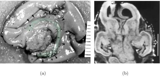
(a) (b)
Figure 2.6: 13 GW. (a) Photography fromKier et al.(1995) in sagittal plane of the medial brain surface of a 13 GW foetus. The frontal lobe is on the left side of the photography and the temporal lobe on the bottom part and the hippocampus is highlighted in green. The corpus callosum is not yet formed. Large ar-rowheads, hippocampal sulcus; small arar-rowheads, the inner limbic arch of the hippocampal formation; OT, olfactory tract. The distance between two grad-uations is 1 mm. (b) Coronal T1-weighted spoiled gradient-echo MR image (45/8/2; 45° flip angle) of an intact 13 GW foetus fromKier et al.(1997). The neocortical parahippocampal gyrus region (P) is small, (T) is the temporal horn. The white vertical line measures 10 mm.
of the hippocampus on 62 foetal Magnetic Resonance Images from 20 to 37 GW with normal neuro-developmental examination at postnatal age. They found a cor-relation between the in-folding angle of the hippocampus and the gestational week. This angle is measured between the line connecting the lateral border of the cornu Ammonis with the medial superior border of the subiculum and the line passing through the midline structures. This angle takes values inferior to 70 degrees for foetuses of less than 25 GW, and superior to 70 degrees for foetuses of more that 30 GW. Okada et al. (2003) investigated the morphological development of the hippocampal formation in children. They showed that this angle increases by
ap-(a) (b)
(c)
Figure 2.7: 16 GW. (a) Photography fromKier et al.(1995) in sagittal plane of the medial brain surface of a 16 GW foetus. Large arrowheads, hippocampal sulcus; small arrowheads, the inner limbic arch of the hippocampal formation; CC, corpus callosum; F, fornix; OT, olfactory tract. The distance between two graduations is 1 mm. (b) Coronal T1-weighted spoiled gradient-echo MR image (45/8/2; 45° flip angle) of intact 13 GW old foetus from Kier et al. (1997). The neo-cortical parahippocampal gyrus region (P) is small. The white vertical line measures 10 mm. (c) coronal histological section (Nissl, original magnification ×24 fromKier et al. (1997)), the CA1 (1), CA2 (2), and CA3 (3) fields of the cornu Ammonis are arranged linearly. The dentate gyrus (small arrowheads) has a tight U-shaped configuration around the CA4 (4) field of the cornu Am-monis. The very thin molecular stratum (M) of the dentate gyrus is separated from the larger molecular stratum of the cornu Ammonis by the very wide hippocampal sulcus (large arrowheads).
Figure 2.8: (A) acetylcholinesterase histochemistry of a 25 GW. (B) a T1-weighted MRI from a 25 GW, and (C), T1-weighted MRI from a full term new born. TH: Thalamus. Images are fromRadoš et al. (2006).
proximately 5° during the 2 first decades after birth, against around 15° during the 17 weeks of gestation observed inRighini et al. (2006). In Okada et al.(2003) they also found that the mean angle was significantly larger for right hippocampus than for left hippocampus, but this result was not replicated in the study ofRighini et al. (2006) on foetuses. Figure 2.8(A) and (B) shows a 25 GW, where we can see that the hippocampus has not achieved its inversion, and in (C) a full term new born in which we can see that the hippocampus has almost terminated its inversion.
Bajic et al. (2010) studied, using an ultra sound modality, the development of the hippocampus in pre-term neonates aged between 23 and 35 GW. They found, in a coronal view, a rounded shape of the hippocampus in 50% of the neonates aged between 23 to 24 GW, in 24% of the neonates aged between 25 to 28 GW and in 14%on the neonates aged between 29 and 36 GW. This rounded shape was mainly
left sided. Therefore, there are already developmental differences between the left hippocampus and the right hippocampus.
2.1.5
Incomplete hippocampal inversion
As we have seen, Baker & Barkovich(1992) observed that during the rotational growth of the telencephalic vesicle, the major portion of the hippocampus is carried dorso-laterally and then ventrally to lie in the medial aspect of the temporal lobe. As the neocortex expands and evolves, the allocortex is displaced inferiorly, medially and internally into the temporal horn. This is why we can observe an inversion of the hippocampus during the development.
There exists a remarkable anatomical variant of the hippocampus which has received various names including "malrotation" and "Incomplete Hippocampal In-version". As proposed in Raininko & Bajic (2010), we use the term "Incomplete Hippocampal Inversion" (IHI) which better describes the incomplete inversion of the hippocampus than the term malrotation. These Incomplete Hippocampal Inversions have been initially observed in healthy subjects by Bronen & Cheung (1991), who showed that the anatomical variant of the hippocampus which presents a rounded shape in a coronal view on MRI ( a criterion to describe these Incomplete Hippocam-pal Inversion) is a normal anatomical variation of the hippocampus. This particular anatomical variation has been mostly observed in patients with epilepsy ((Lehéricy et al., 1995;Baulac et al.,1998)). In these studies they describe hippocampi with a rounded shape in a coronal view in MRI, a protruding collateral sulcus and a medial position of the hippocampus as shown in Figure 2.9. Barsi et al. (2000) wondered
Figure 2.9: Coronal point of view of hippocampi, the 3 images are from the same subject, the top image shows the heads of the hippocampi, the middle image shows the bodies of hippocampi and the bottom one, the tails. The left hippocam-pus framed in red presents a rounded shape, a medial positioning and a deep colateral sulcus which are typical criteria for an IHI.
if this particular hippocampal shape has a developmental origin since they observe these IHI in subjects with corpus callosum agenesis. Finally, some studies demon-strate that this anatomical variant of the hippocampus, which mainly presents a rounded or vertical shape, a medial positioning and a deep collateral sulcus, has in fact a developmental origin (Righini et al.,2006; Bajic et al., 2010).
IHI have been mostly observed and studied in pathological cases such as epilepsy (Lehéricy et al. (1995), Barsi et al. (2000), Baulac et al. (1998), Bernasconi et al. (2005), Peltier et al. (2005), Stiers et al. (2010), Bajic et al. (2009), Friedman & Tandon(2013)) or congenital brain malformations (Donmez et al.(2009),Sato et al. (2001), Baker & Barkovich (1992)). These studies found very different frequencies
of IHI. In Barsi et al. (2000), they found 6% of IHI in a population composed of 597 patients with suspicion of epilepsy 69% of the IHI were left-sided, 19% right-sided and 12% bilateral. In Peltier et al. (2005), 14% of 97 epileptic patients had IHI. InBernasconi et al. (2005), 43% of the 30 temporal lobe epileptic patients had IHI, and 49% of 76 patients with malformations of cortical development had IHI. In Bajic et al. (2009), 30% of the 201 patients with epilepsy had IHI, 67% of the IHI were left-sided, 7% right-sided and 27% bilateral. For the developmental brain malformations,Baker & Barkovich(1992) found IHI in 36% of 36 patients,Sato et al. (2001) found IHI in 64% of 44 patients and Donmez et al.(2009) 56% of IHI for 62 patients. These frequencies of IHI are different because of the chosen populations, but also because the criteria used to identify IHI are not identical, therefore do not allow reproducible or comparable results.
Some studies tried to determinate the frequency in the normal population. InBernasconi et al. (2005) they found 10% of IHI in 50 healthy controls. In Peltier et al. (2005),
IH were found in 6% of the control population composed of 50 subjects including 11 patients without epilepsy but including other pathologies. InBajic et al. (2009) authors used 150 subjects including 116 patients, and found 18% of IHI, mostly left-sided. In one study (Bronen & Cheung, 1991) authors found that 21% of the 29 volunteers had a shape different than the usual flat appearance as the right hippocampus on Figure 2.9.
The limitations of these studies are that they not only include healthy controls but also patients without epilepsy nor developmental brain malformations but with various conditions; the size of the populations used which makes difficult a good
estimation of the frequency of IHI; the criteria used are not the same.
2.2
Visualisation in MRI
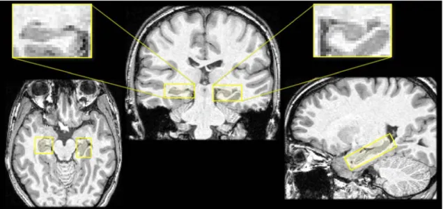
In vivo, the first choice of imaging techniques to observe brain structures as the hippocampus is Magnetic Resonance Images (MRI) with 3D T1-weighted sequences, with roughly 1mm isotropic resolution (Figure2.10(a)). T1-weighted MRI measures the time of longitudinal relaxation (T1) i.e. the time needed by the hydrogen atoms (present in large quantities in molecules of biological tissues) to recover their initial balance after excitation by a magnetic field (1.5 or 3 Tesla in general), this time is different depending on the tissue property. Hypo-signal indicates liquids such as cerebro-spinal fluid and blood, the gray matter is in dark gray and the white matter in light gray. This sequence allows a good overview in 3 dimensions of the anatomical structures of the brain. Figure 2.10(a) shows three views (from left to right) axial, coronal and sagittal of the hippocampus on a 3D T1-weighted MRI. These three views allow to show the medial positioning of the hippocampus and its global elongated shape. They also allow a visualisation in 3 dimensions of the neighbouring structures, and a good overview of the whole brain. But this MRI sequence do not allow the identification of finer details of the hippocampus, as the cornu Ammonis or the gyrus dentatus; only the fimbria can be seen (in white in T1 MRI) but not clearly in every image.
It is also possible to use other MRI sequences such as the T2-weighted spin echo sequences to observe a particular structure or to detect variations of contrast in a tissue. This sequence measures the time of transversal relaxation (T2) which is
(a) T1-weighted with resolution1mm× 1mm × 1mm
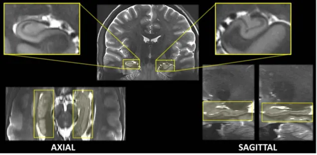
(b) T2-weighted with resolution 0.3mm× 0.3mm × 4mm
Figure 2.10: Two visualizations of hippocampus of a same subject from the IRMA7 database. (a) Magnetic Resonance Images with a T1-weighted acquisition and (b) T2-weighted acquisition. Views are (from left to right) axial, coronal and sagittal.
the time required for the spins (of the hydrogen atoms) to return to their phase coherence due to the spin-spin interactions. Hypo-signal indicates blood and air, the cerebro-spinal fluid is in hyper-signal, the white matter is in dark gray and the gray matter in light gray. This MRI sequence provides a better contrast of the inner structures of the hippocampus, but does not allow an isotropic resolution because of the acquisition time. In Figure 2.10(b), the sequence was acquired to have a good resolution in the coronal plane around the hippocampus. We can see a coronal view (in the middle) of the hippocampus: the cornu Ammonis, the gyrus dentatus, the hippocampus sulcus and even the alveus are clearly identifiable. Due to the anisotropic resolution, the axial and sagittal views are very difficult to interpret and do not permit a representation in three dimensions of any structure.
It is also possible to have an ultra-high resolution of the hippocampus in coronal view, with a good resolution in axial and sagittal, by using several T2-weighted sequences at 7 Tesla. Then a registration method is applied to these MRIs to co-register all sequences in order to obtain a good resolution in axial and sagittal. In Figure 2.11, we can observe the registration of different T2-weighted MR images at 7T (Marrakchi et al., submitted paper), on the same subject as in Figure 2.10. Figure2.11allows a good 3D visualization of the hippocampus subfields; the sagittal view shows the fimbria which is the dark line over the hippocampus, and as in the axial view one can observe the hippocampal sulcus which separates the cornu Ammonis from the gyrus dentatus. But the acquisition of such MRI is not always available since this is a reserche sequence and there is in France only two centre equipped by 7T systems adapted for humans.
Figure 2.11: Visualization of the hippocampi of a same subject of the IRMA7 database in Figure 2.10. The volumetric image have been computed by Marrakchi et al. (submitted paper) from different T2-weighted sequence in 7T MRI, by registering the different acquisition using the 3T MRI.
We can see in all these images (figures 2.10 and2.11) that the left hippocampus of the subject presents an incomplete hippocampal inversion.
The 3D T1 weighted MRI sequence allows a good visualization of the external boundaries of the hippocampus and to form large databases, which is exactly what we need to analysis the shape of the hippocampus.
2.3
Role
The medial part of the temporal lobe receives input from different regions. The perirhinal cortex and the parahippocampal cortex receive the information from the neocortical areas. These cortex are inter-connected and connected to the
entorhi-nal cortex which is itself the principal source of afferents of the hippocampus. The perirhinal and the parahippocampal cortex receive the efferents from the hippocam-pus and the entorhinal cortex and then project on the associative cortex. These structures are more than a simple interface for the communication between the hip-pocampal formation and the neocortical areas, these structures play a key role in the memorisation processes.
2.3.1
Memory
The term "memory" groups together different concepts and processes. The infor-mation processing is different according to the quantity of inforinfor-mation to integrate and to the type of information. Alvarez & Squire(1994) developed a theory of the consolidation of the mnesic marks which supposes that the consolidation process starts when the informations coming from different sensory modalities are linked between each other under the form of a mnesic mark by the hippocampus and oth-ers structures of the temporal lobe. Nadel & Moscovitch (2001) and Nadel et al. (2000) proposed a different theory which is based on multiple mnesic marks. The hippocampus is a need for the recovery of episodic memories requiring a spatial context.
The different types of memories are listed below. A review of all memory types can be found inTulving (1995).
Short term memory This mnesic system contains the working memory, and is a limited mnesic system in terms of capacity. This system keeps in memory
informations needed for a short term processing.
Long term memory This a mnesic system not limited in capacities, which allows the processing of informations from anterior learnings kept in memory. Long term memory can be divided in two types of memories: declarative (or explicit) memory and implicit memory.
Implicit memory This is a non-conscious process which permits the acquisition of motor abilities as riding a bike.
Declarative memory This memory requires the use of the temporal lobe, and is a conscious process. This mnesic system is based on informations that can be declared and are accessible to the conscience. Declarative memory can be divided into semantic memory and episodic memory.
Semantic memory This is the memory of general informations. This is the memory of the words, ideas and knowledge on the world regardless of the temporo-spatial information, without reference to the learning context.
Episodic memory According to Wheeler et al. (1997), episodic memory allows to mentally travel in time, and to consciously have a representation of past events to integrate them into a future project. This mnesic system allows the storage and the recovery of personal events situated in their temporal and spatial context.
The study of patients who have suffered brain lesions has made a significant contribution to the understanding of memory processes. First of all, this is the study of the famous amnesic patient known as H.M. which allowed a better under-standing of the implication of temporal lobes in memories. H.M. was epileptic since childhood and to reduce its seizures, in adulthood he finally underwent a bilateral resection (in 1953) of its hippocampi, amygdala and a part of the neighbouring cor-tex (Scoville & Milner, 1957). After his surgery, H.M. lost his capability to form new long term memories. He was able to remind a sequence of words, but he forgot this sequence after stopping saying it. Furthermore, he lost the memory of events that happened during the three years before the resection. On the other hand, his procedural and implicit memories were intact. The many studies on this patient (Corkin, 2002; Squire, 2009) allow to conclude that short term memory, long term memory, procedural memory and declarative memory processes are different. These studies also showed the role of the temporal lobes in the consolidation of new infor-mations in declarative memory, that is a long process since memory of years before the resection were lost. The declarative memory seems to be blocked by the ab-sence of hippocampi. An other patient named K.C. and presented in the study of Tulving (2002), suffered a cranial trauma in 1981 at the age of 30. The MRI of his brain showed bilateral hippocampal lesions, but the sub-hippocampal structures were spared during the resection. K.C. cannot recollect any personal events whereas his semantic knowledge is intact: he knows many facts about himself and can learn new factual informations without any episodic memories. He can not imagine his future any more than he can remember the past. Unlike H.M., his semantic
mem-ory is preserved as his sub-hippocampal structures, and like H.M. he suffered very severe damage to his episodic memory. As suggested in Rosenbaum et al. (2005) and Tulving(2002), a distinction can be made between the hippocampi which play a critical role in episodic memory and the sub-hippocampal structures which appear to be more involved in semantic memory. This theory has been exposed in other works as inVargha-Khadem et al.(1997) andWarrington(1975) with other patients with brain lesions.
2.3.2
Spatial navigation
Hippocampi also plays a role in spatial memory and navigation. In animal stud-ies as in rats or mice (O’Keefe & Dostrovsky, 1971), they found that hippocampi present a type of neurons that becomes active when the rat enters in a particu-lar place in the environment. These neurons are named place cells and have been identified in humans by Ekstrom et al. (2003). Furthermore the study of Maguire et al. (2000) on the taxi drivers of London, before the appearance of Global Po-sitioning System (GPS), showed that the gray matter of the posterior part of the hippocampus was larger in taxi drivers than in control subjects, but in the anterior part of the hippocampus the gray matter was larger in control subjects than in taxi drivers. Authors also found a correlation between the amount of time an individual worked as a taxi driver and the volume of gray matter of the posterior and ante-rior part of the hippocampus. An other study on the role of hippocampi (Burgess et al., 2002), showed that the visualization of spatial scenes in virtual reality in-volves the parahippocampal gyrus. The right hippocampus seems to be involved in
memory for locations within an environment whereas the left hippocampus seems to be involved in context-dependant episodic memory or in autobiographical memory (Burgess et al.,2002;Maguire, 2001).
2.3.3
Pathologies
We will make a short description of the main pathologies in which the hippocam-pus is involved.
Figure 2.12: Hippocrates
Temporal Lobe Epilepsy The first document
about epilepsy dates from 2000 BC: epilepsy is de-scribed as a supernatural characteristic, since the sick persons were thought to be under the influence of a god. Even if Hippocrates suggests in a treatise, in 400 BC, that this sacred disease is not spiritual but a dis-ease caused by a brain impairment (and named it the grand mal (great disease)), it is only from the 17-18th century that epilepsy was considered as a neurological disease.
Now epilepsy is considered as a brain disorder characterized by generalized or focal epileptic seizures. Among the different forms of focal epilepsies, the most frequent is temporal lobe epilepsy (TLE), which is present is around 40% of cases (Engel Jr,1996). Seizures generally start in the hippocampus (Spencer et al.,1990) and continue during one or two minutes with or without alteration of
conscious-ness. The association between hippocampal abnormalities and TLE is well-known, hippocampal sclerosis (atrophy of the hippocampus with altered signal intensity in MRI) is a frequent finding in patients with TLE (Eriksson et al.,2008). Even if it is not yet clear whether epilepsy is caused by hippocampal abnormalities, or whether the hippocampus is damaged by cumulative effects of seizures, TLE is resistant to medications in 89% of cases when patients present hippocampal sclerosis, in 75% of cases when patients present a malformation of cortical development and in 97% of cases of malformation of cortical development and hippocampal sclerosis (Semah et al., 1998). In carefully selected patients, epilepsy surgery can effectively con-trol seizures as shown in Wiebe et al. (2001). MRI plays an important role in the pre-surgical evaluation to determine the presence or not of atrophy, since in case of atrophy, more than 70% of surgically treated TLE patients achieve to be seizures free after surgery (Wiebe et al., 2001; Wiebe, 2003). On the other hand, one case of resection of an hippocampal malformation has been reported in Dericioglu et al. (2009).
Alzheimer’s Disease In the antiquity, Greeks and Romans associated old age with mental decline (Berchtold & Cotman, 1998), but it is in 1901 that the psy-chiatrist Alois Alzheimer described the first case in a fifty-year-old woman of what became known as Alzheimer’s disease. He publicly reported this case after the death of the patient on 1906.
Alzheimer’s disease (AD) is a neuro-degenerative disorder (progressive loss of neurons) which mainly causes impairment of memory, and disorientation followed by other cognitive symptoms. AD patients present two types of lesions caused by