HAL Id: hal-01344074
https://hal.archives-ouvertes.fr/hal-01344074
Submitted on 11 Jul 2016
HAL is a multi-disciplinary open access
archive for the deposit and dissemination of
sci-entific research documents, whether they are
pub-lished or not. The documents may come from
teaching and research institutions in France or
abroad, or from public or private research centers.
L’archive ouverte pluridisciplinaire HAL, est
destinée au dépôt et à la diffusion de documents
scientifiques de niveau recherche, publiés ou non,
émanant des établissements d’enseignement et de
recherche français ou étrangers, des laboratoires
publics ou privés.
Embarrassingly Parallel Search
Jean-Charles Régin, Mohamed Rezgui, Arnaud Malapert
To cite this version:
Jean-Charles Régin, Mohamed Rezgui, Arnaud Malapert. Embarrassingly Parallel Search. 19th
International Conference on Principles and Practice of Constraint Programming (CP 2013), Sep 2013,
Uppsala, Sweden. �10.1007/978-3-642-40627-0_45�. �hal-01344074�
Embarrassingly parallel search
Jean-Charles R´egin, Mohamed Rezgui and Arnaud Malapert
Universit´e Nice-Sophia Antipolis, I3S UMR 6070, CNRS, France
[email protected], [email protected], [email protected]
Abstract. We propose the Embarrassingly Parallel Search, a simple and effi-cient method for solving constraint programming problems in parallel. We split the initial problem into a huge number of independent subproblems and solve them with available workers (i.e., cores of machines). The decomposition into subproblems is computed by selecting a subset of variables and by enumerating the combinations of values of these variables that are not detected inconsistent by the propagation mechanism of a CP Solver. The experiments on satisfaction problems and on optimization problems suggest that generating between thirty and one hundred subproblems per worker leads to a good scalability. We show that our method is quite competitive with the work stealing approach and able to solve some classical problems at the maximum capacity of the multi-core ma-chines. Thanks to it, a user can parallelize the resolution of its problem without modifying the solver or writing any parallel source code and can easily replay the resolution of a problem.
1
Introduction
There are two mainly possible ways for parallelizing a constraint programming solver. On one hand, the filtering algorithms (or the propagation) are parallelized or distributed. The most representative work on this topic has been carried out by Y. Hamadi [5]. On the other hand, the search process is parallelized. We will focus on this method. For a more complete description of the methods that have been tried for using a CP solver in parallel, the reader can refer to the survey of Gent et al. [4].
When we want to use k machines for solving a problem, we can split the initial prob-lem into k disjoint subprobprob-lems and give one subprobprob-lem to each machine. Then, we gather the different intermediate results in order to produce the results corresponding to the whole problem. We will call this method: simple static decomposition method. The advantage of this method is its simplicity. Unfortunately, it suffers from several draw-backs that arise frequently in practice: the times spent to solve subproblems are rarely well balanced and the communication of the objective value is not good when solving an optimization problem (the workers are independent). In order to equilibrate the sub-problems that have to be solved some works have been done about the decomposition of the search tree based on its size [8,3,7]. However, the tree size is only approximated and is not strictly correlated with the resolution time. Thus, as mentioned by Bordeaux et al. [1], it is quite difficult to ensure that each worker will receive the same amount of work. Hence, this method suffers from some issues of scalability, since the resolution time is the maximum of the resolution time of each worker. In order to remedy for these
issues, another approach has been proposed and is currently more popular: the work stealing idea.
The work stealing idea is quite simple: workers are solving parts of the problem and when a worker is starving, it ”steals” some work from another worker. Usually, it is implemented as follows: when a worker W has no longer any work, it asks another worker V if it has some work to give it. If the answer is positive, then the worker V splits the problem it currently solves into two subproblems and gives one of them to the starving worker W . If the answer is negative then W asks another worker U , until it gets some work to do or all the workers have been considered.
This method has been implemented in a lot of solvers (Comet [10] or ILOG Solver [12] for instance), and into several ways [14,6,18,2] depending on whether the work to be done is centralized or not, on the way the search tree is split (into one or several parts), or on the communication method between workers.
The work stealing approach partly resolves the balancing issue of the simple static decomposition method, mainly because the decomposition is dynamic. Therefore, it does not need to be able to split a problem into well balanced parts at the beginning. However, when a worker is starving it has to avoid stealing too many easy problems, because in this case, it have to ask for another work almost immediately. This happens frequently at the end of the search when a lot of workers are starving and ask all the time for work. This complicates and slows down the termination of the whole search by increasing the communication time between workers. Thus, we generally observe that the method scales well for a small number of workers whereas it is difficult to maintain a linear gain when the number of workers becomes larger, even thought some methods have been developed to try to remedy for this issue [16,10].
In this paper, we propose another approach: the embarrassingly parallel search (EPS) which is based on the embarrassingly parallel computations [15].
When we have k workers, instead of trying to split the problem into k equivalent subparts, we propose to split the problem into a huge number of subproblems, for in-stance 30k subproblems, and then we give successively and dynamically these sub-problems to the workers when they need work. Instead of expecting to have equivalent subproblems, we expect that for each worker the sum of the resolution time of its sub-problems will be equivalent. Thus, the idea is not to decompose a priori the initial problem into a set of equivalent problems, but to decompose the initial problem into a set of subproblems whose resolution time can be shared in an equivalent way by a set of workers. Note that we do not know in advance the subproblems that will be solved by a worker, because this is dynamically determined. All the subproblems are put in a queue and a worker takes one when it needs some work.
The decomposition into subproblems must be carefully done. We must avoid sub-problems that would have been eliminated by the propagation mechanism of the solver in a sequential search. Thus, we consider only problems that are not detected inconsis-tent by the solver.
The paper is organized as follows. First, we recall some principles about embarrass-ingly parallel computations. Next, we introduce our method for decomposing the initial problems. Then, we give some experimental results. At last, we make a conclusion.
2
Preliminaries
2.1 A precondition
Our approach relies on the assumption that the resolution time of disjoint subproblems is equivalent to the resolution time of the union of these subproblems. If this condition is not met, then the parallelization of the search of a solver (not necessarily a CP Solver) based on any decomposition method, like simple static decomposition, work stealing or embarrassingly parallel methods may be unfavorably impacted.
This assumption does not seem too strong because the experiments we performed do not show such a poor behavior with a CP Solver. However, we have observed it in some cases with a MIP Solver.
2.2 Embarrassingly parallel computation
A computation that can be divided into completely independent parts, each of which can be executed on a separate process(or), is called embarrassingly parallel [15].
For the sake of clarity, we will use the notion of worker instead of process or pro-cessor.
An embarrassingly parallel computation requires none or very little communication. This means that workers can execute their task, i.e. any communication that is without any interaction with other workers.
Some well-known applications are based on embarrassingly parallel computations, like Folding@home project, Low level image processing, Mandelbrot set (a.k.a. Frac-tals) or Monte Carlo Calculations [15].
Two steps must be defined: the definition of the tasks (TaskDefinition) and the task assignment to the workers (TaskAssignment). The first step depends on the application, whereas the second step is more general. We can either use a static task assignment or a dynamic one.
With a static task assignment, each worker does a fixed part of the problem which is known a priori.
And with a dynamic task assignment, a work-pool is maintained that workers con-sult to get more work. The work pool holds a collection of tasks to be performed. Work-ers ask for new tasks as soon as they finish previously assigned task. In more complex work pool problems, workers may even generate new tasks to be added to the work pool.
In this paper, we propose to see the search space as a set of independent tasks and to use a dynamic task assignment procedure. Since our goal is to compute one solution, all solutions or to find the optimal solution of a problem, we introduce another operation which aims at gathering solutions and/or objective values:TaskResultGathering. In this step, the answers to all the sub-problems are collected and combined in some way to form the output (i.e. the answer to the initial problem).
For convenience, we create a master (i.e. a coordinator process) which is in charge of these operations: it creates the subproblems (TaskDefinition), holds the work-pool and assigns tasks to workers (TaskAssignment) and fetches the computations made by the workers (TaskResultGathering).
In the next parts, we will see how the three operations can be defined in order to be able to run the search in parallel and in an efficient way.
3
Problem decomposition
3.1 Principles
We have seen that decomposing the initial problem into the same number of subprob-lems as workers may cause unbalanced resolution time for each worker. Thus, our idea is to strongly increase the number of considered subproblems, in order to define an embarrassingly parallel computation leading to good performance.
Before going into further details on the implementation, we would like to establish a property. While solving a problem, we will call:
– active time of a worker the sum of the resolution times of a worker (the decompo-sition time is excluded).
– inactive time of a worker the difference between the elapsed time for solving all the subproblems (the decomposition time is excluded) and the active time of the worker.
Our approach is mainly based on the following remark:
Remark 1 The active time of all the workers may be well balanced even if the resolu-tion time of each subproblem is not well balanced
The main challenge of a static decomposition is not to define equivalent problems, it is to avoid some workers without work whereas some others are running. We do not need to know in advance the resolution time of each subproblem. We just expect that the workers will have equivalent activity time. In order to reach that goal we propose to decompose the initial problem into a lot of subproblems. This increases our chance to obtain well balanced activity times for the workers, because we increase our chance to be able to obtain a combination of resolution times leading to the same activity time for each worker.
For instance, when the search space tends to be not equilibrated, we will have sub-problems that will take a longer time to be solved. By having a lot of subsub-problems we increase our chance to split these subproblems into several parts having comparable resolution time and so to obtain a well balanced load of the workers at the end. It also reduces the relative importance of each subproblem with respect to the resolution of the whole problem.
Here is an example of the advantage of using a lot of subproblems. Consider a prob-lem which requires 140s to be solved and that we have 4 workers. If we split the probprob-lem into 4 subproblems then we have the following resolution times: 20, 80, 20, 20. We will need 80s to solve these subproblems in parallel. Thus, we gain a factor of 140/80 = 1.75. Now if we split again each subproblem into 4 subproblems we could obtain the following subproblems represented by their resolution time: ((5, 5, 5, 5), (20, 10, 10, 40), (2, 5, 10, 3), (2, 2, 8, 8)). In this case, we could have the following assignment: worker1 : 5+20+2+8 = 35; worker2 : 5+10+2+10 = 27; worker3 : 5+10+5+3+2+8 = 33
and worker4 : 5 + 40 = 45. The elapsed time is now 45s and we gain a factor of 140/45 = 3.1. By splitting again the subproblems, we will reduce the average res-olution time of the subproblems and expect to break the 40s subproblem. Note that decomposing more a subproblem does not increase the risk of increasing the elapsed time.
Property 1 Let P be an optimization problem, or a satisfaction problem for which we search for all solutions. IfP is split into subproblems whose maximum resolution time istmax, then
(i) the minimum resolution time of the whole problem is tmax
(ii) the maximum inactivity time of a worker is less than or equal to tmax. Suppose that a worker W has an inactivity time which is greater than tmax. Consider the moment where W started to wait after its activity time. At this time, there is no more available subproblems to solve, otherwise W would have been active. All active workers are then finishing their last task, whose resolution is bounded by tmax. Thus, the remaining resolution time of each of these other workers is less than tmax. Hence a contradiction.
3.2 Subproblems generation
Suppose we want to split a problem into q disjoint subproblems. Then, we can use several methods.
A simple method We can proceed as follows: 1. We consider any ordering of the variables x1,...xn.
2. We define by Akthe Cartesian product D(x1) × ... × D(xk).
3. We compute the value k such that |Ak−1| < q ≤ |Ak|.
Each assignment of Akdefines a subproblem and so Akis the sought decomposition.
This method works well for some problems like the n-queen or the golomb ruler, but it is really bad for some other problems, because a lot of assignments of A may be trivially not consistent. Consider for instance that x1, x2and x3have the three values
{a, b, c} in their domains and that there is an alldiff constraint involving these three variables. The Cartesian product of the domains of these variables contains 27 tuples. Among them only 6 ((a, b, c), (a, c, b), (b, a, c),(b, c, a),(c, a, b), (c, b, a)) are not incon-sistent with the alldiff constraint. That is, only 6/27 = 2/9 of the generated problems are not trivially inconsistent. It is important to note that most of these inconsistent prob-lems would never be considered by a sequential search. For some probprob-lems we have observed more than 99% of the generated problems were detected inconsistent by run-ning the propagation. Thus, we present another method to avoid this issue.
Not Detected Inconsistent (NDI) subproblems We propose to generate only subprob-lems that are not detected inconsistent by the propagation. The generation of q such subproblems becomes more complex because the number of NDI subproblems may be not related to the Cartesian product of some domains. A simple algorithm could be to perform a Breadth First Search (BFS) in the search tree, until the desired number of NDI subproblems is reached. Unfortunately, it is not easy to perform efficiently a BFS mainly because a BFS is not an incremental algorithm like a Depth First Search (DFS). Therefore, we propose to use a process similar to an iterative deepening depth-first search [9]: we repeat a Depth-bounded Depth First Search (DBDFS), in other words a DFS which never visits nodes located at a depth greater than a given value, increasing the bound until generating the right number of subproblems. Each branch of a search tree computed by this search defines an assignment. We will denote by NDIk the set
of assignments computed for the depth k. For generating q subproblems, we repeat the DBDFS until we reach a level k such that |NDIk−1| < q ≤ |NDIk|. For convenience
and simplicity, we use a static ordering of the variables. We improve this method in three ways:
1. We try to estimate some good values for k in order to avoid repeating too many DBDFS. For instance, if for a given depth u we produce only q/1000 subproblems and if the size of the domains of the three next non assigned variables is 10, then we can deduce that we need to go at least to the depth u + 3.
2. In order to avoid repeating the same DFS for the first variables while repeating DBDFS, we store into a table constraint the previous computed assignments. More precisely, if we have computed NDIkthen we use a table constraint containing all
these assignments when we look for NDIlwith l > k.
3. We parallelize our decomposition algorithm in a simple way. Consider we have w workers. We search for w NDI subproblems. Then, each worker receives one of these subproblems and decomposes it into q/w NDI subproblems by using our algorithm. The master gathers all computed subproblems. If a worker is not able to generate q/w subproblems because it solves its root NDI problem by decomposing it, the master asks the workers to continue to decompose their subproblems into smaller ones until reaching the right number of subproblems. Note that the load balancing of the decomposition is not really important because once a worker has finished its decomposition work it begins to solve the available subproblems.
Large Domains Our method can be adapted to large domains. A new step must be introduced in the algorithm in the latest iteration. If the domain of the latest considered variable, denoted by lx, is large then we cannot consider each of its values individually. We need to split its domain into a fix number of parts and use each part as a value. Then, either the desired number of subproblems is generated or we have not been able to reach that number. In this latter case, we need to split again the domain of lx, for instance by splitting each part into two new parts (this multiplies by at most 2 the number of generated subproblems) and we check if the generated number of subproblems is fine or not. This process is repeated until the right number of subproblems is generated or the domain of lx is totally decomposed, that is each part corresponds to a value. In this latter case, we continue the algorithm by selecting a new variable.
3.3 Implementation Satisfaction Problems
– TheTaskDefinitionoperation consists of computing a partition of the initial problem P into a set S of subproblems.
– TheTaskAssignmentoperation is implemented by using a FIFO data structure (ie a queue). Each time a subproblem is defined it is added to the back of the queue. When a worker needs some work it takes a subproblem from the queue.
– TheTaskResultGatheringoperation is quite simple : when searching for a solution it stops the search when one is found; when searching for all solutions, it just gathers the solutions returned by the workers.
Optimization Problems
In case of optimization problems we have to manage the best value of the objective function computed so far. Thus, the operations are slightly modified.
– TheTaskDefinitionoperation consists of computing a partition of the initial problem P into a set S of subproblems.
– TheTaskAssignmentoperation is implemented by using a queue. Each time a sub-problem is defined it is added to the back of the queue. The queue is also associated with the best objective value computed so far. When a worker needs some work, the master gives it a subproblem from the queue. It also gives it the best objective value computed so far.
– TheTaskResultGatheringoperation manages the optimal value found by the worker and the associated solution.
Note that there is no other communication, that is when a worker finds a better solution, the other workers that are running cannot use it for improving their current resolution. So, if the absence of communication may increase our performance, this aspect may also lead to a decrease of performance. Fortunately, we do not observe this bad behavior in practice. We can see here another argument for having a lot of subproblems in case of optimization problems: the resolution of a subproblem should be short for improving the transmission of a better objective value and for avoiding performing some work that could have been ignored with a better objective value.
3.4 Size of the partition
One important question is: how many subproblems do we generate?
This is mainly an experimental question. However, we can notice that if we want to have a good scalability then this number should be defined in relation to the number of workers that are involved. More precisely, it is more consistent to have q subproblems per worker than a total of q subproblems.
3.5 Replay
One interesting advantage of our method in practice is that we can simply replay a resolution in parallel by saving the order in which the subproblems have been executed. This costs almost nothing and helps a lot the debugging of applications.
4
Related Work
The decomposition of some hard parts of the problem into several subproblems in order to fill a work-pool has been proposed by [10] in conjunction with the work-stealing approach.
Yun and Epstein proposed to parallelize a sequential solver in order to find one solution for a satisfaction problem [17]. Their approach strongly relies on a weight learning mechanism and on the use of a restart strategy. A first portfolio phase allows to initialize the weights as well as solving easy problems. In the splitting phase, the manager distributes subproblems to the worker with a given search limit. If the worker is not able to solve the problem within the limit, it returns the problem to the manager for further partitioning by iterative bisection partitioning.
We can already notice three major differences with our approach. First, we partition statically the problems at the beginning of the search whereas they use an on-demand dynamic partitioning. Second, there is much more communication between the manager and the workers since the workers have to notify the manager of encountered search limit. Last, the same part of the search tree can be explored several times since the worker do not learn clauses form the unsuccessful runs. Therefore, it really complicated to adapt their approach for solution enumeration whereas it is straightforward with ours.
5
Experiments
Machines All the experiments have been made on a Dell machine having four E7-4870 Intel processors, each having 10 cores with 256 GB of memory and running under Scientific Linux.
Our experiments can be reproduced by downloading the program EPSearch for Linux from [13].
Solvers We implemented our method on the top of two CP solvers: or-tools rev2555 by Google and Gecode 4.0.0 (http://www.gecode.org/).
Experimental Protocol Our code just performs three operations:
1. It reads a FlatZinc model or the model is directly created with the API of the solver. 2. It creates the threads and defines an instance of the solver for each thread
3. It computes the subproblems, feeds the threads with them and gathers the results.
For each problem, we will either search for all solutions of satisfaction problems or solve the whole optimization problem (i.e. find the best solution and prove its optimal-ity). The resolution times represent the elapsed time to solve the whole problem that is they include the decomposition time and the times needed by the workers to solve subproblems.
Note that testing the performance of a parallel method is more complex with an optimization problem because the chance may play a role. It can advantage or disad-vantage us. However, in the real life, optimization problems are quite common therefore it is important to test our method on them.
Selected Benchmarks We selected a wide range of problems that are representative of the types of problems solved in CP. Some are coming from the CSP lib and have been modeled by Hakan Kjellerstrandk (http://www.hakank.org/) and some are coming from the MiniZinc distribution (1.5 see [11]). We selected instances that are not too easy (ie more than 20s) and that are not too long to be solved (ie in less than 3600s) with the Gecode solver.
1. The examples coming from Hakan Kjellerstrandk are: golombruler-13; magicsequence-40000; sportsleague-10; warehouses (number of warehouses = 10, number of stores = 20 and a fixed cost = 180); setcovering (Placing of fire stations with 80 cities and a min distance fixed at 24); allinterval-15 (the model of Regin and Puget of the CSP Lib is used);
2. The Flatzinc instances coming from the MiniZinc distribution are: 2DLevelPack-ing (5-20-6), depotPlacement (att48-5; rat99-5), fastfood (58), openStacks (01-problem-15-15;01-wbp-30-15-1), sugiyama (2-g5-7-7-7-7-2), patternSetMining (k1-german-credit), sb-sb (13-13-6-4), quasigroup7-10, non-non-fast-6, radiation-03, bacp-7, talent-scheduling-alt-film116.
Tests We will denote by #sppw, the number of subproblems per worker. We will study the following aspects of our method:
5.1 the scalability compared to other static decompositions
5.2 the inactivity time of the workers as a function of the value of #sppw 5.3 the difficulty of the subproblems when dealing with a huge number of them 5.4 the advantage of parallelizing the decomposition
5.5 the influence of the value of #sppw on the factor of improvements 5.6 its performance compared to the work-stealing approach
5.7 the influence of the CP solver that is used 5.1 Comparison with a simple static decomposition
We consider the famous n-queens problem, because it is a classical benchmark and because some proposed methods [6,1] were not able to observe a factor greater than 29 with a simple static decomposition of the problems even when using 64 workers. Figure 1 shows that our method scales very well when #sppw is greater than 20. The limit of the scalability (a maximum ratio of 29) described in [1] clearly disappeared. Note that we used the same search strategy as in [1] and two 40-cores Dell machines for this experiment.
5.2 Ratio of NDI subproblems
Figure 2 shows the percentage of NDI problems generated by the simple method of decomposition for all problems. We can see that this number depends a lot on the con-sidered instances. For some instances, the number is close to 100% whereas for some others it can be really close to 0% which indicates a decomposition issue. The mean starts at 55% and decreases according to the number of subproblems to end at 1%. Most of the inconsistent problems generated by the simple decomposition method would not have been considered by a sequential search. Therefore, for some instances this method should not be used. This is the reason why we do not generate any non NDI problems.
0 10 20 30 40 50 60 70 80 10 20 30 40 50 60 70 80 Speedup #workers 10 20 50 100
Fig. 1. 17-queens: performance as a function of #sppw (10,20,50 and 100). We no longer observe the limit of a gain factor of 29.
0 0.2 0.4 0.6 0.8 1 400 800 2000 4000 12000 40000 120000 NDI Problems
Fig. 2. Percentage of NDI problems generated by the simple decomposition method for all prob-lems. The geometric mean is in bold, dashed lines represent minimum and maximum values, and the area filled in gray is the geometric standard deviation is filled in gray.
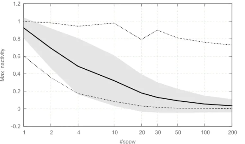
5.3 The inactivity time as a function of #sppw -0.2 0 0.2 0.4 0.6 0.8 1 1.2 1 2 4 10 20 30 50 100 200 Max inactivity #sppw
Fig. 3. Percentage of maximum inactivity time of the workers (geometric mean).
Figure 3 shows that the percentage of the maximum inactivity time of the workers decreases when the number of subproblems per worker is increased. From 20 subprob-lems per worker, we observe that in average the maximum inactivity time represents less than 20% of the resolution time
5.4 Parallelism of the decomposition
0 0.1 0.2 0.3 0.4 0.5 0.6 0.7 0.8 0.9 1 10 20 30 50 100 300 1000 3000 10000
decomp. over solving times
#sppw Sequential
Parallel
Figure 4 compares the percentage of total time needed to decompose the problem when only the master performs this operation or when the workers are also involved. We clearly observe that the parallelization of the decomposition saves some time, especially for a large number of subproblems per worker.
5.5 Influence of the number of considered subproblems
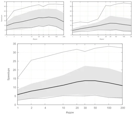
0 5 10 15 20 25 30 35 1 2 4 10 20 30 50 100 200 Speedups #sppw 0 5 10 15 20 25 30 35 1 2 4 10 20 30 50 100 200 #sppw 0 5 10 15 20 25 30 35 1 2 4 10 20 30 50 100 200 Speedups #sppw
Fig. 5. Speed up as a function of the number of subproblems for finding all solutions of satis-faction problems (top left), for finding and proving the optimality of optimization problems (top right) and for all the problems (bottom).
Figure 5 describes the speed up obtained by the Embarrassignly Parallel Search (EPS) as a function of the number of subproblems for Gecode solver. The best results are obtained with a number subproblems per worker between 30 and 100. In other words, we propose to start the decomposition with q = 30w, where w is the number of workers.
It is interesting to note that a value of #sppw in [30,100] is good for all the consid-ered problems and seems independent from them.
The reduction of the performance when increasing the value of #sppw comes from the fact that the decomposition process solves an increasing part of the problem; and this process is slower than a resolution procedure.
Note that with our method, only 10% of the resolution time is lost if we use a sequential decomposition instead of a parallel one.
5.6 Comparison with the work stealing approach
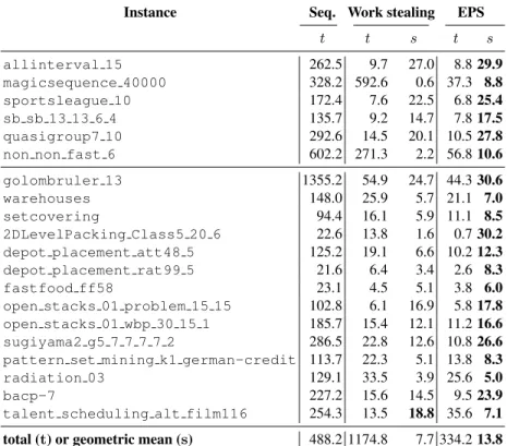
Instance Seq. Work stealing EPS
t t s t s allinterval 15 262.5 9.7 27.0 8.8 29.9 magicsequence 40000 328.2 592.6 0.6 37.3 8.8 sportsleague 10 172.4 7.6 22.5 6.8 25.4 sb sb 13 13 6 4 135.7 9.2 14.7 7.8 17.5 quasigroup7 10 292.6 14.5 20.1 10.5 27.8 non non fast 6 602.2 271.3 2.2 56.8 10.6 golombruler 13 1355.2 54.9 24.7 44.3 30.6 warehouses 148.0 25.9 5.7 21.1 7.0 setcovering 94.4 16.1 5.9 11.1 8.5 2DLevelPacking Class5 20 6 22.6 13.8 1.6 0.7 30.2 depot placement att48 5 125.2 19.1 6.6 10.2 12.3 depot placement rat99 5 21.6 6.4 3.4 2.6 8.3 fastfood ff58 23.1 4.5 5.1 3.8 6.0 open stacks 01 problem 15 15 102.8 6.1 16.9 5.8 17.8 open stacks 01 wbp 30 15 1 185.7 15.4 12.1 11.2 16.6 sugiyama2 g5 7 7 7 7 2 286.5 22.8 12.6 10.8 26.6 pattern set mining k1 german-credit 113.7 22.3 5.1 13.8 8.3 radiation 03 129.1 33.5 3.9 25.6 5.0 bacp-7 227.2 15.6 14.5 9.5 23.9 talent scheduling alt film116 254.3 13.5 18.8 35.6 7.1 total (t) or geometric mean (s) 488.2 1174.8 7.7 334.2 13.8 Table 1. Resolution with 40 workers, and #sspw=30 using Gecode 4.0.0. Column t contains the resolution time in seconds and column s contains the speed-ups. The last row shows the sum of the resolution times and the geometric mean of the speed-ups.
Table 1 presents a comparison between the EPS and the work stealing method avail-able in Gecode. The geometric average gain factor with the work stealing method is 7.7 (7.8 for satisfaction problems and 7.6 for optimization problems) whereas with the EPS it is 13.8 (18.0 for satisfaction problems and 12.3 for optimization problems). Our method improves the work stealing approach in all cases but one.
5.7 Influence of the CP Solver
Instance Seq. EPS t t s allinterval 15 2169.7 67.7 32.1 magicsequence 40000 – – – sportsleague 10 – – – sb sb 13 13 6 4 227.6 18.1 12.5 quasigroup7 10 – – –
non non fast 6 2676.3 310.0 8.6 golombruler 13 16210.2 573.6 28.3
warehouses – – –
setcovering 501.7 33.6 14.9 2DLevelPacking Class5 20 6 56.2 3.6 15.5 depot placement att48 5 664.9 13.7 48.4 depot placement rat99 5 67.0 2.8 23.7 fastfood ff58 452.4 25.1 18.0 open stacks 01 problem 15 15 164.7 7.1 23.2 open stacks 01 wbp 30 15 1 164.9 6.3 26.0 sugiyama2 g5 7 7 7 7 2 298.8 20.5 14.6 pattern set mining k1 german-credit 270.7 12.8 21.1 radiation 03 416.6 23.5 17.7
bacp-7 759.7 23.8 32.0
talent scheduling alt film116 575.7 15.7 36.7 total (t) or geometric mean (s) 25677.2 1158.1 21.3 Table 2. Resolution with 40 workers, and #sspw=30 using or-tools (revision 2555).
We also performed some experiments by using or-tools solver. With or-tools the speed up of the EPS are increased (See Table 2). We obtain a geometric average gain factor of 13.8 for the Gecode solver and 21.3 for or-tools.
6
Conclusion
In this paper we have presented the Embarrassingly Parallel Search (EPS) a simple method for solving CP problems in parallel. It proposes to decompose the initial prob-lem into a set of k subprobprob-lems that are not detected inconsistent and then to send them to workers in order to be solved. After some experimentations, it appears that split-ting the initial problem into 30 such subproblems per worker gives an average factor of gain equals to 21.3 with or-tools and 13.8 with Gecode while searching for all the solutions or while finding and proving the optimality, on a machine having 40 cores. This is competitive with the work stealing approach.
Acknowledgments. We would like to thank very much Laurent Perron and Claude Michel for their comments which helped improve the paper.
References
1. Lucas Bordeaux, Youssef Hamadi, and Horst Samulowitz. Experiments with massively par-allel constraint solving. In Craig Boutilier, editor, IJCAI, pages 443–448, 2009.
2. Geoffrey Chu, Christian Schulte, and Peter J. Stuckey. Confidence-based work stealing in parallel constraint programming. In Ian P. Gent, editor, CP, volume 5732 of Lecture Notes in Computer Science, pages 226–241. Springer, 2009.
3. G´erard Cornu´ejols, Miroslav Karamanov, and Yanjun Li. Early estimates of the size of branch-and-bound trees. INFORMS Journal on Computing, 18(1):86–96, 2006.
4. Ian P. Gent, Chris Jefferson, Ian Miguel, Neil C.A. Moore, Peter Nightingale, Patrick Prosser, and Chris Unsworth. A preliminary review of literature on parallel constraint solving,. In Proceedings PMCS-11 Workshop on Parallel Methods for Constraint Solving, 2011. 5. Youssef Hamadi. Optimal distributed arc-consistency. Constraints, 7:367–385, 2002. 6. Joxan Jaffar, Andrew E. Santosa, Roland H. C. Yap, and Kenny Qili Zhu. Scalable distributed
depth-first search with greedy work stealing. In ICTAI, pages 98–103. IEEE Computer So-ciety, 2004.
7. Philip Kilby, John K. Slaney, Sylvie Thi´ebaux, and Toby Walsh. Estimating search tree size. In AAAI, pages 1014–1019, 2006.
8. Donald E. Knuth. Estimating the efficiency of backtrack programs. Mathematics of Compu-tation, 29:121–136, 1975.
9. R. Korf. Depth-first iterative-deepening: An optimal admissible tree search. Artificial Intel-ligence, 27:97109, 1985.
10. Laurent Michel, Andrew See, and Pascal Van Hentenryck. Transparent parallelization of constraint programming. INFORMS Journal on Computing, 21(3):363–382, 2009.
11. MiniZinc. http://www.g12.csse.unimelb.edu.au/minizinc/, 2012.
12. Laurent Perron. Search procedures and parallelism in constraint programming. In Joxan Jaf-far, editor, CP, volume 1713 of Lecture Notes in Computer Science, pages 346–360. Springer, 1999.
13. Jean-Charles Rgin. www.constraint-programming.com/people/regin/papers.
14. Christian Schulte. Parallel search made simple. In Nicolas Beldiceanu, Warwick Harvey, Martin Henz, Franois Laburthe, Eric Monfroy, Tobias Mller, Laurent Perron, and Christian Schulte, editors, Proceedings of TRICS: Techniques foR Implementing Constraint program-ming Systems, a post-conference workshop of CP 2000, Singapore, September 2000. 15. B. Wilkinson and M. Allen. Parallel Programming: Techniques and Application Using
Net-worked Workstations and Parallel Computers. Prentice-Hall Inc., 2nd edition edition, 2005. 16. Feng Xie and Andrew J. Davenport. Massively parallel constraint programming for su-percomputers: Challenges and initial results. In Andrea Lodi, Michela Milano, and Paolo Toth, editors, CPAIOR, volume 6140 of Lecture Notes in Computer Science, pages 334–338. Springer, 2010.
17. Xi Yun and Susan L. Epstein. A hybrid paradigm for adaptive parallel search. In CP, pages 720–734, 2012.
18. Peter Zoeteweij and Farhad Arbab. A component-based parallel constraint solver. In Rocco De Nicola, Gian Luigi Ferrari, and Greg Meredith, editors, COORDINATION, volume 2949 of Lecture Notes in Computer Science, pages 307–322. Springer, 2004.