HAL Id: inria-00316195
https://hal.inria.fr/inria-00316195v2
Submitted on 22 Apr 2009
HAL is a multi-disciplinary open access
archive for the deposit and dissemination of
sci-entific research documents, whether they are
pub-lished or not. The documents may come from
L’archive ouverte pluridisciplinaire HAL, est
destinée au dépôt et à la diffusion de documents
scientifiques de niveau recherche, publiés ou non,
émanant des établissements d’enseignement et de
Experimental Study of the HUM Control Operator for
Linear Waves
Gilles Lebeau, Maëlle Nodet
To cite this version:
Gilles Lebeau,
Maëlle Nodet.
Experimental Study of the HUM Control Operator for
Linear Waves.
Experimental Mathematics, Taylor & Francis, 2010, 19 (1), pp.93-120.
�10.1080/10586458.2010.10129063�. �inria-00316195v2�
Experimental Study of the HUM Control
Operator for Linear Waves
Gilles Lebeau
∗†Universit´
e de Nice
Ma¨
elle Nodet
‡Universit´
e de Grenoble, INRIA
April 21, 2009
Abstract
We consider the problem of the numerical approximation of the lin-ear controllability of waves. All our experiments are done in a bounded domain Ω of the plane, with Dirichlet boundary conditions and internal control. We use a Galerkin approximation of the optimal control operator of the continuous model, based on the spectral theory of the Laplace op-erator in Ω. This allows us to obtain surprisingly good illustrations of the main theoretical results available on the controllability of waves, and to formulate some questions for the future analysis of optimal control theory of waves.
∗Laboratoire J.-A. Dieudonn´e, Parc Valrose, Nice, France, [email protected] †Institut Universitaire de France
‡Laboratoire J. Kuntzmann, Domaine Universitaire, Grenoble, France,
Contents
1 Introduction 3
2 The analysis of the optimal control operator 5
2.1 The optimal control operator . . . 5
2.2 Theoretical results . . . 8
2.3 The spectral Galerkin method . . . 12
2.4 Computation of the discrete control operator . . . 16
3 Numerical setup and validation 18 3.1 Geometries and control domains . . . 18
3.2 Time and space smoothing . . . 18
3.3 Validation of the eigenvalues computation . . . 19
3.4 Reconstruction error. . . 19
3.5 Validation for the square geometry . . . 19
3.5.1 Finite differences versus exact eigenvalues . . . 19
3.5.2 Impact of the number of eigenvalues . . . 21
4 Numerical experiments 21 4.1 Frequency localization . . . 21
4.2 Space localization . . . 22
4.2.1 Dirac experiments . . . 22
4.2.2 Box experiments in the square . . . 22
4.3 Reconstruction error . . . 23
4.4 Energy of the control function . . . 23
4.5 Condition number . . . 24 4.6 Non-controlling domains . . . 25 Acknowledgement 25 References 26 List of Figures 28 List of Tables 67
1
Introduction
This paper is devoted to the experimental study of the exact controlla-bility of waves. All our experiments will be done in a bounded domain Ω of the plane, with Dirichlet boundary conditions and with internal con-trol. We use the most natural approach for the numerical computation: a Galerkin approximation of the optimal control operator of the continuous model based on the spectral theory of the Laplace operator in Ω. This will allow us to obtain surprisingly good illustrations of the main theoretical results available on the controllability of waves, and to formulate some questions for the future analysis of the optimal control theory of waves.
The problem of controllability for linear evolution equations and sys-tems has a long story for which we refer to the review of D.-L. Russel in [Rus78] and to the book of J. L. Lions [Lio88]. Concerning controllabil-ity of linear waves, the main theoretical result is the so called “Geomet-ric Control Condition” of C. Bardos, G. Lebeau and J. Rauch [BLR92],
GCCin short, which gives a (almost) necessary and sufficient condition
for exact controllability. This is a “geometrical optics” condition on the behavior of optical rays inside Ω. Here, optical rays are just straight lines inside Ω, reflected at the boundary according to the Snell-Descartes law of reflection. The precise definition of optical rays near points of tangency
with the boundary is given in the works of R. Melrose and J. Sj¨ostrand
[MS78] and [MS82]. For internal control, GCC asserts that waves in a regular bounded domain Ω are exactly controllable by control functions supported in the closure of an open sub-domain U and acting during a time T , if (and only if, if one allows arbitrary small perturbations of the time control T and of the control domain U )
GCC: every optical ray of length T in Ω enters the sub-domain U . Even when GCC is satisfied, the numerical computation of the con-trol is not an easy task. The original approach consists first in discretizing the continuous model, and then in computing the control of the discrete system to use it as a numerical approximation of the continuous one. This method has been developed by R. Glowinski et al. (see [GLL90] and [GHL08]), and used for numerical experiments in [AL98]. However, as observed in the first works of R. Glowinski, interaction of waves with a numerical mesh produces spurious high frequency oscillations. In fact, the discrete model is not uniformly exactly controllable when the mesh size goes to zero, since the group velocity converges to zero when the solutions wavelength is comparable to the mesh size. In other words, the processes of numerical discretization and observation or control do not commute. A precise analysis of this lack of commutation and its impact on the com-putation of the control has been done by E. Zuazua in [Zua02] and [Zua05]. In this paper, we shall use another approach, namely we will dis-cretize the optimal control of the continuous model using a projection of the wave equation onto the finite dimensional space spanned by the
conditions, −△ej= ω2
jej, ej|∂Ω=0, with ωj≤ ω. Here, ω will be a cutoff
frequency at our disposal. We prove (see lemma 2 in section 2.3) that when GCC is satisfied, our numerical control converges when ω → ∞ to the optimal control of the continuous model . Moreover, when GCC is not satisfied, we will do experiments and we will see an exponential blow-up in the cutoff frequency ω of the norm of the discretized optimal control. These blow-up rates will be compared to theoretical results in section 2.3.
The paper is organized as follows.
Section 2 is devoted to the analysis of the optimal control operator for
waves in a bounded regular domain of Rd. In section 2.1, we recall the
definition of the optimal control operator Λ. In section 2.2, we recall some known theoretical results on Λ: existence, regularity properties and the fact that it preserves the frequency localization. We also state our first conjecture, namely that the optimal control operator Λ is a microlocal operator. In section 2.3, we introduce the spectral Galerkin
approxima-tion MT,ω−1 of Λ, where ω is a cutoff frequency. We prove the convergence
of MT,ω−1 toward Λ when ω → ∞, and we analyze the rate of this
conver-gence. We also state our second conjecture on the blow-up rate of M−1
T,ω when GCC is not satisfied. Finally, in section 2.4, we introduce the basis of the energy space in which we compute the matrix of the operator MT,ω. Section 3 is devoted to the experimental validation of our Galerkin approximation. In section 3.1 we introduce the 3 different domains of the plane for our experiments: square, disc and trapezoid. In the first two cases, the geodesic flow is totally integrable and the exact eigenfunctions and eigenvalues of the Laplace operator with Dirichlet boundary condi-tion are known. This is not the case for the trapezoid. In seccondi-tion 3.2 we introduce the two different choices of the control operator we use in our
ex-periments. In the first case (non smooth case), we use χ(t, x) = 1[0,T ]1U.
In the second case (smooth case), we use a suitable regularization of the first case (see formulas (66) and (67)). Perhaps the main contribution of this paper is to give an experimental evidence that the choice of a smooth enough control operator is the right way to get accuracy on control com-puting. In section 3.3, in the two cases of the square and the disc, we compare the exact eigenvalues with the eigenvalues computed using the 5-points finite difference approximation of the Laplace operator. In sec-tion 3.4, formula (69), we define the reconstrucsec-tion error of our method. Finally, in section 3.5, in the case of the square geometry, we compare the control function (we choose to reconstruct a single eigenvalue) when the eigenvalues and eigenvectors are computed either with finite differences or with exact formulas, and we study the experimental convergence of our numerical optimal control to the exact optimal control of the continuous model when the cutoff frequency goes to infinity.
The last section, 4, presents various numerical experiments which il-lustrate the theoretical results of section 2, and are in support of our two
conjectures. In section 4.1, our experiments illuminate the fact that the optimal control operator preserves the frequency localization, and that this property is far much stronger when the control function is smooth, as predicted by theoretical results. In section 4.2, we use Dirac and box experiments to illustrate the fact that the optimal control operator shows a behavior very close to the behavior of a pseudo-differential operator: this is in support of our first conjecture. In section 4.3, we plot the re-construction error as a function of the cutoff frequency: this illuminates how the rate of convergence of the Galerkin approximation depends on the regularity of the control function. In section 4.4, we present various results on the energy of the control function. In section 4.5, we compute
the condition number of the matrix MT,ωfor a given control domain U , as
a function of the control time T and the cutoff frequency ω. In particular, figures 31 and 32 are in support of our second conjecture on the blow-up
rate of M−1
T,ω when GCC is not satisfied. In section 4.6, we perform
ex-periments in the disc when GCC is not satisfied, for two different data: in the first case, every optical rays of length T starting at a point where the data is not small enters the control domain U , and we observe a rather good reconstruction error if the cutoff frequency is not too high. In the second case, there exists an optical ray starting at a point where the data is not small and which never enters the control domain, and we observe a very poor reconstruction at any cutoff frequency. This is a fascinating phenomena which has not been previously studied in theoretical works. It will be of major practical interest to get quantitative results on the best cutoff frequency which optimizes the reconstruction error (this optimal cutoff frequency is equal to ∞ when GCC is satisfied, the reconstruction error being equal to 0 in that case), and to estimate the reconstruction er-ror at the optimal cutoff frequency. Clearly, our experiments indicate that a weak Geometric Control Condition associated to the data one wants to reconstruct will enter in such a study.
2
The analysis of the optimal control
op-erator
2.1
The optimal control operator
Here we recall the basic facts we will need in our study of the optimal control operator for linear waves. For more details on the HUM method, we refer to the book of J.-L. Lions [Lio88].
In the framework of the wave equation in a bounded open subset Ω of
Rdwith boundary Dirichlet condition, and for internal control the problem
of controllability is stated in the following way. Let T be a positive time, U a non void open subset of Ω, and χ(t, x) as follows:
χ(t, x) = ψ(t)χ0(x) (1)
where χ0 is a real L∞ function on Ω, such that support(χ0) = U and
on ]0, T [. For a given f = (u0, u1) ∈ H1
0(Ω) ×L2(Ω), the problem is to find
a source v(t, x) ∈ L2(0, T ; L2(Ω)) such that the solution of the system
8 < : ¤u = χv in ]0, +∞[×Ω u|∂Ω= 0, t > 0 (u|t=0, ∂tu|t=0) = (0, 0) (2)
reaches the state f = (u0, u1) at time T . We first rewrite the wave oper-ator in (2) as a first order system. Let A be the matrix
iA =„ 0 Id
△ 0
«
(3)
Then A is a unbounded self-adjoint operator on H = H1
0(Ω) × L2(Ω),
where the scalar product on H01(Ω) is
R
Ω∇u∇vdx and D(A) = {u =
(u0, u1) ∈ H, A(u) ∈ H, u0|∂Ω = 0}. Let λ = √−△D where −△D
is the canonical isomorphism from H01(Ω) onto H−1(Ω). Then λ is an
isomorphism from H1
0(Ω) onto L2(Ω). The operator B(t) given by
B(t) = „ 0 0 χ(t, .)λ 0 « (4) is bounded on H, and one has
B∗(t) =„0 λ
−1χ(t, .)
0 0
«
(5) The system (2) is then equivalent to
(∂t− iA)f = B(t)g, f (0) = 0 (6)
with f = (u, ∂tu), g = (λ−1v, 0). For any g(t) ∈ L1([0, ∞[, H), the
evolution equation
(∂t− iA)f = B(t)g, f (0) = 0 (7)
admits a unique solution f = S(g) ∈ C0([0, +∞[, H) given by the Duhamel
formula
f (t) =
Z t
0
ei(t−s)AB(s)g(s)ds (8)
Let T > 0 be given. Let RT be the reachable set at time T
RT= {f ∈ H, ∃g ∈ L2([0, T ], H), f = S(g)(T )} (9)
Then RT is a linear subspace of H, and is the set of states of the system
that one can reach in time T , starting from rest, with the action of an
L2 source g filtered by the control operator B. The control problem
con-sists in giving an accurate description of RT, and exact controllability is
equivalent to the equality RT= H. Let us recall some basic facts.
Let H = L2([0, T ], H). Let F be the closed subspace of H spanned by
solutions of the adjoint evolution equation
Observe that, in our context, A∗ = A, and the function h in (10) is
given by h(t) = e−i(T −t)AhT. Let B∗ be the adjoint of the operator
g 7→ S(g)(T ). Then B∗is the bounded operator from H into H defined
by
B∗(hT)(t) = B∗(t)e−i(T −t)AhT (11)
For any g ∈ L2([0, T ], H), one has, with fT = S(g)(T ) and h(s) =
e−i(T −s)AhT the fundamental identity
(fT|hT)H =
Z T
0
(B(s)g(s)|h(s))ds = (g|B∗(hT))H (12)
From (12), one gets easily that the following holds true
RT is a dense subspace of H ⇐⇒ B∗is an injective operator (13)
which shows that approximate controllability is equivalent to a uniqueness result on the adjoint equation. Moreover, one gets from (12), using the Riesz and closed graph theorems, that the following holds true
RT = H ⇐⇒ ∃C, khk ≤ CkB∗hk ∀h ∈ H (14)
This is an observability inequality, and B∗is called the observability
op-erator. We rewrite the observability inequality (14) in a more explicit form
∃C, khk2H≤ C
Z T
0
kB∗(s)e−i(T −s)Ahk2Hds ∀h ∈ H (15)
Assuming that (15) holds true, then RT = H, Im(B∗) is a closed
subspace of H, and B∗ is an isomorphism of H onto Im(B∗). For any
f ∈ H, let Cf be the set of control functions g driving 0 to f in time T
Cf = g ∈ L2([0, T ], H), f = ZT 0 ei(T −s)AB(s)g(s)ds ff (16) From (12), one gets
Cf = g0+ (ImB∗)⊥, g0∈ ImB∗∩ Cf (17)
and g0 = B∗hT is the optimal control in the sense that
min{kgkL2([0,T ],H), g ∈ Cf} is achieved at g = g0 (18)
Let Λ : H → H, Λ(f) = hT be the control map, so that the optimal
control g0 is equal to g0(t) = B∗(t)e−i(T −t)AΛ(f ). Then Λ is exactly the
inverse of the map MT : H → H with
MT = Z T 0 m(T − t)dt = Z T 0 m(s)ds
m(s) = eisAB(T − s)B∗(T − s)e−isA∗
(19)
Observe that m(s) = m∗(s) is a bounded, self-adjoint, non-negative
oper-ator on H. Exact controllability is thus equivalent to
∃C > 0, MT= Z T 0 ei(T −t)A„0 0 0 χ2(t, .) «
With Λ = M−1
T , the optimal control is then given by g0(t) = B∗(t)e−i(T −t)AΛ(f )
and is by (5) of the form g0= (λ−1χ∂tw, 0) where w(t) = e−i(T −t)AΛ(f )
is the solution of
¤w = 0 in R× Ω, w|∂Ω= 0
(w(T, .), ∂tw(T, .)) = Λ(f ) (21)
Thus, the optimal control function v in (2) is equal to v = χ∂tw, where
w is the solution of the dual problem (21). The operator Λ = MT−1, with
MT given by (20) is called the optimal control operator.
2.2
Theoretical results
In this section we recall some theoretical results on the analysis of the optimal control operator Λ. We will assume here that Ω is a bounded
open subset of Rd with smooth boundary ∂Ω, and that any straight line
in Rdhas only finite order of contacts with the boundary. In that case,
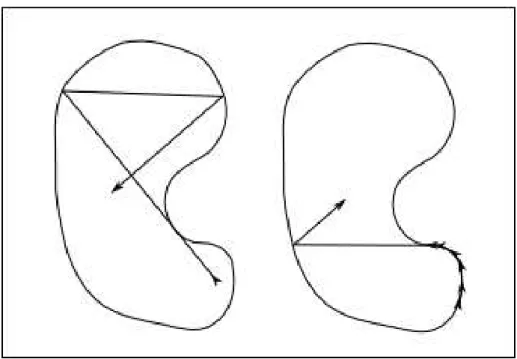
optical rays are uniquely defined. See an example of such rays in figure 1. [Figure 1 about here.]
Let M = Ω × Rt. The phase space is
bT∗M = T∗
M \ T∂M∗ ≃ T∗M ∪ T∗∂M.
The characteristic variety of the wave operator is the closed subset Σ
ofbT∗M of points (x, t, ξ, τ ) such that |τ| = |ξ| when x ∈ Ω and |τ| ≥ |ξ|
when x ∈ ∂Ω. LetbS∗Ω be the set of points
bS∗
Ω = {(x0, ξ0), with |ξ0| = 1 if x0∈ Ω, |ξ0| ≤ 1 if x0 ∈ ∂Ω}
For ρ0 = (x0, ξ0) ∈ bS∗Ω, and τ = ±1, we shall denote by s →
(γρ0(s), t − sτ, τ ), s ∈ R the generalized bicharacteristic ray of the wave
operator, issued from (x0, ξ0, t, τ ). For the construction of the
Melrose-Sj¨ostrand flow, we refer to [MS78], [MS82] and to [H¨or85], vol 3, chapter
XXIV . Then s → γρ0(s) = (x(ρ0, s), ξ(ρ0, s)) is the optical ray starting
at x0 in the direction ξ0. When x0 ∈ ∂Ω and |ξ0| < 1, then the right
(respectively left) derivative of x(ρ0, s) at s = 0 is equal to the unit vector
in Rdwhich projects on ξ0∈ T∗∂Ω and which points inside (respectively
outside) Ω. In all other cases, x(ρ0, s) is derivable at s = 0 with derivative
equal to ξ0.
We first recall the theorem of [BLR92], which gives the existence of the operator Λ:
Theorem 1 If the geometric control condition GCC holds true, then MT
is an isomorphism.
Next, we recall some new theoretical results obtained in [DL09]. For these results, the choice of the control function χ(t, x) in (1) will be es-sential.
Definition 1 The control function χ(t, x) = ψ(t)χ0(x) is smooth if χ0∈
For s ∈ R, we denote by Hs(Ω, △) the domain of the operator (−△Dirichlet)s/2.
One has H0(Ω, △) = L2(Ω), H1(Ω, △) = H01(Ω), and if (ej)j≥1 is an L2
orthonormal basis of eigenfunctions of −△ with Dirichlet boundary
con-ditions, −△ej= ω2
jej, 0 < ω1≤ ω2≤ ..., one has
Hs(Ω, △) = {f ∈ D′(Ω), f =X
j
fjej, X
j
ωj2s|fj|2< ∞} (22)
The following result of [DL09] says that, under the hypothesis that the control function χ(t, x) is smooth, the optimal control operator Λ preserves the regularity:
Theorem 2 Assume that the geometric control condition GCC holds
true, and that the control function χ(t, x) is smooth. Then the optimal
control operator Λ is an isomorphism of Hs+1(Ω, ∆) ⊕ Hs(Ω, ∆) for all
s ≥ 0.
Observe that theorem 1 is a particular case of theorem 2 with s = 0. In our experimental study, we will see in section 4.3 that the regularity of the control function χ(t, x) is not only a nice hypothesis to get theo-retical results. It is also very efficient to get accuracy in the numerical computation of the control function. In other words, the usual choice of
the control function χ(t, x) = 1[0,T ]1U is a very poor idea to compute a
control.
The next result says that the optimal control operator Λ preserves the frequency localization. To state this result we briefly introduce the
mate-rial needed for the Littlewood-Paley decomposition. Let φ ∈ C∞([0, ∞[),
with φ(x) = 1 for |x| ≤ 1/2 and φ(x) = 0 for |x| ≥ 1. Set ψ(x) =
φ(x) − φ(2x). Then ψ ∈ C∞
0 (R∗), ψ vanishes outside [1/4, 1], and one has
φ(s) + ∞ X
k=1
ψ(2−ks) = 1, ∀s ∈ [0, ∞[
Set ψ0(s) = φ(s) and ψk(s) = ψ(2−ks) for k ≥ 1. We then define the
spectral localization operators ψk(D), k ∈ N, in the following way: for
u =P jajej, we define ψk(D)u =X j ψk(ωj)ajej (23) One hasP
kψk(D) = Id and ψi(D)ψj(D) = 0 for |i − j| ≥ 2. In addition,
we introduce Sk(D) = k X j=0 ψj(D) = ψ0(2−kD), k ≥ 0 (24)
Obviously, the operators ψk(D) and Sk(D) acts as bounded operators on
H = H1
Theorem 3 Assume that the geometric control condition GCC holds true, and that the control function χ(t, x) is smooth. There exists C > 0 such that for every k ∈ N, the following inequality holds true
kψk(D)Λ − Λψk(D)kH≤ C2−k
kSk(D)Λ − ΛSk(D)kH≤ C2−k (25)
Theorem 3 states that the optimal control operator Λ, up to lower or-der terms, acts individually on each frequency block of the solution. For
instance, if en is the n-th eigenvector of the orthonormal basis of L2(Ω),
if one drives the data (0, 0) to (en, 0) in (2) using the optimal control, both the solution u and control v in equation (2) will essentially live at
frequency ωn for n large. We shall do experiments on this fact in section
4.1, and we will clearly see the impact of the regularity of the control func-tion χ(t, x) on the accuracy of the frequency localizafunc-tion of the numerical control.
Since by the above results the optimal control operator Λ preserves the regularity and the frequency localization, it is very natural to expect that Λ is in fact a micro-local operator, and in particular preserves the wave front set. For an introduction to micro-local analysis and
pseudo-differential calculus, we refer to [Tay81] and [H¨or85]. In [DL09], it is
proved that the optimal control operator Λ for waves on a compact Rie-mannian manifold without boundary is in fact an elliptic 2 × 2 matrix of pseudo-differential operators. This is quite an easy result, since if χ(t, x)
is smooth the Egorov theorem implies that the operator MT given by
(20) is a 2 × 2 matrix of pseudo-differential operators. Moreover, the
ge-ometric control condition GCC implies easily that MT is elliptic. Since
MT is self adjoint, the fact that MT is an isomorphism follows then from
Ker(MT) = {0}, which is equivalent to the injectivity of B∗. This is
proved in [BLR92] as a consequence of the uniqueness theorem of Calderon for the elliptic second order operator △. Then it follows that its inverse
Λ = MT−1is an elliptic pseudo-differential operator.
In our context, for waves in a bounded regular open subset Ω of Rd
with boundary Dirichlet condition, the situation is far much complicated, since there is no Egorov theorem in the geometric setting of a manifold
with boundary. In fact, the Melrose-Sj¨ostrand theorem [MS78], [MS82]
on propagation of singularities at the boundary (see also [H¨or85], vol 3,
chapter XXIV for a proof) implies that the operator MT given by (20)
is a microlocal operator, but this is not sufficient to imply that its
in-verse Λ is micro-local. However let ρ0 = (x0, ξ0) ∈ T∗Ω, |ξ0| = 1 be a
point in the cotangent space such that the two optical rays defined by
the Melrose-Sj¨ostrand flow (see [MS78], [MS82]) s ∈ [0, T ] → γ±ρ0(s) =
(x(±ρ0, s), ξ(±ρ0, s)), with ±ρ0 = (x0, ±ξ0), starting at x0 in the
direc-tions ±ξ0 have only transversal intersections with the boundary. Then it
is not hard to show using formula (20) and the parametrix of the wave operator, inside Ω and near transversal reflection points at the boundary
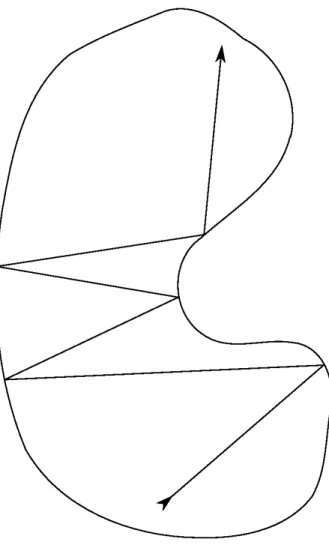
∂Ω, as presented in figure 2, that MT is microlocally at ρ0an elliptic 2 × 2
[Figure 2 about here.]
More precisely, let J be the isomorphism from H1
0⊕ L2on L2⊕ L2given by J = 1 2 „ λ −i λ i « (26)
One has 2kJuk2L2⊕L2 = kuk2
H1
0⊕L
2, and if u(t, x) is the solution of the
wave operator 2u = 0 with Dirichlet boundary conditions on ∂Ω, and
Cauchy data at time t0 equal to (u0, u1), then one has
λu(t, .) = λ cos((t − t0)λ)u0+ sin((t − t0)λ)u1
= ei(t−t0)λ “ λu0−iu1 2 ” + e−i(t−t0)λ “ λu0+iu1 2 ” (27)
so the effect of the isomorphism J is to split the solution u(t, x) into a sum of two waves with positive and negative temporal frequency. Moreover, one has JeitAJ−1= „ eitλ 0 0 e−itλ « (28)
Then JMTJ−1 acts as a non negative self-adjoint operator on L2⊕ L2,
and is equal to JMTJ−1= 12 „ Q+ −T −T∗ Q− « Q±= RT 0 e
±isλχ2(T − s, .)e∓isλds
T = RT
0 e
isλχ2(T − s, .)eisλds
(29)
From (29), using the parametrix of the wave operator, inside Ω and near transversal reflection points at the boundary ∂Ω, and integration by parts to show that T is a smoothing operator, it is not difficult to get that
JMTJ−1 is microlocally at ρ0 ∈ T∗Ω a pseudo-differential operator of
order zero with principal symbol
σ0(JMTJ−1)(ρ0) =1 2 „ q+(x0, ξ0) 0 0 q−(x0, ξ0) « q±(x0, ξ0) =RT 0 χ 2(T − s, x(±ρ0, s))ds (30)
Obviously, condition (GCC) guarantees that σ0(JMTJ−1)(ρ0) is elliptic,
and therefore JΛJ−1 will be at ρ0 a pseudo-differential operator of order
zero with principal symbol
σ0(JΛJ−1)(ρ0) = 2 „ q−1+ (x0, ξ0) 0 0 q−1− (x0, ξ0) « (31) Therefore, the only difficulty in order to prove that Λ is a microlocal operator is to get a precise analysis of the structure of the operator MT
near rays which are tangent to the boundary. Since the set of ρ ∈bS∗Ω for
which the optical ray γρ(s) has only transversal points of intersection with
the boundary is dense in T∗Ω \ T∂Ω∗ (see [H¨or85]), it is not surprising that
our numerical experiments in section 4.2 (where we compute the optimal
control associated to a Dirac mass δx0, x0 ∈ Ω), confirms the following
Conjecture 1 Assume that the geometric control condition GCC holds true, that the control function χ(t, x) is smooth, and that the optical rays have no infinite order of contact with the boundary. Then Λ is a microlocal operator.
Of course, part of the difficulty is to define correctly what is a mi-crolocal operator in our context. In the above conjecture, mimi-crolocal will implies in particular that the optimal control operator Λ preserves the wave front set. A far less precise information is to know that Λ is a mi-crolocal operator at the level of mimi-crolocal defect measures, for which we refer to [G´er91]. But this is an easy by-product of the result of N. Burq and G. Lebeau in [BL01].
2.3
The spectral Galerkin method
In this section we describe our numerical approximation of the optimal control operator Λ, and we give some theoretical results on the numerical
approximation MT,ω of the operator MT given by (20), even in the case
where the geometric control condition GCC is not satisfied.
For any cutoff frequency ω, we denote by Πωthe orthogonal projection,
in the Hilbert space L2(Ω), on the finite dimensional linear subspace L2
ω
spanned by the eigenvectors ej for ωj ≤ ω. By the Weyl formula, if cd
denotes the volume of the unit ball in Rd, one has
N (ω) = dim(L2ω) ≃ (2π)−dVol(Ω)cdωd (ω → +∞) (32)
Obviously, Πω acts on H = H1
0× L2 and commutes with eitA, λ and
J. We define the Galerkin approximation MT,ω of the operator MT as
the operator on L2 ω× L2ω MT,ω= ΠωMTΠω= Z T 0 ei(T −t)AΠω„0 0 0 χ2(t, .) «
Πωe−i(T −t)Adt (33)
Obviously, the matrix MT,ωis symmetric and non negative for the Hilbert
structure induced by H on L2ω× L2ω, and by (19) one has with nω(t) =
B∗(t)Πωe−i(T −t)A
MT,ω=
Z T
0
n∗ω(t)nω(t)dt (34)
By (29) one has also
JMT,ωJ−1= 1 2 „ Q+,ω −Tω −T∗ ω Q−,ω « Q±,ω= RT 0 e ±isλΠωχ2 (T − s, .)Πωe∓isλds Tω= RT 0 e isλΠωχ2 (T − s, .)Πωeisλds (35)
Let us first recall two easy results. For convenience, we recall here
the proof of these results. The first result states that the matrix MT,ω is
always invertible.
Lemma 1 For any (non zero) control function χ(t, x), the matrix MT,ω
Proof. Let u = (u0, u1) ∈ L2
ω× L2ω such that MT,ω(u) = 0. By (34)
one has
0 = (MT,ω(u)|u)H =
Z T
0
knω(t)(u)k2Hdt.
This implies nω(t)(u) = 0 for almost all t ∈]0, T [. If u(t, x) is the solution
of the wave equation with Cauchy data (u0, u1) at time T , we thus get
by (5) and (1) ψ(t)χ0(x)∂tu(t, x) = 0 for t ∈ [0, T ], and since ψ(t) > 0 on ]0, T [ and χ0(x) > 0 on U , we get ∂tu(t, x) = 0 on ]0, T [×U. One has
u0=P ωj≤ωajej(x), u1= P ωj≤ωbjej(x) and ∂tu(t, x) = X ωj≤ω
ωjajsin((T − t)ωj)ej(x) + X
ωj≤ω
bjcos((T − t)ωj)ej(x)
Thus we getP
ωj≤ωωjajej(x) =
P
ωj≤ωbjej(x) = 0 for x ∈ U, which
implies, since the eigenfunctions ejare analytic in Ω, that aj= bj= 0 for
all j. 2
For any ω0≤ ω, we define Π⊥
ω = 1 − Πω, and we set
kΠ⊥ωΛΠω0kH = rΛ(ω, ω0)
kΠ⊥ωMTΠω0kH= rM(ω, ω0)
(36)
Since the ranges of the operators ΛΠω0 and MTΠω0 are finite dimensional
vector spaces, one has for any ω0
limω→∞rΛ(ω, ω0) = 0
limω→∞rM(ω, ω0) = 0 (37)
The second result states that when GCC holds true, the inverse matrix
M−1
T,ω converges in the proper sense to the optimal control operator Λ
when the cutoff frequency ω goes to infinity.
Lemma 2 Assume that the geometric condition GCC holds true. There
exists c > 0 such that the following holds true: for any given f ∈ H, let
g = Λ(f ), fω= Πωf and gω= M−1
T,ω(fω). Then, one has
kg − gωkH≤ ckf − fωkH+ kΛ(fω) − MT,ω−1(fω)kH (38) with lim ω→∞kΛ(fω) − M −1 T,ω(fω)kH= 0 (39)
Proof. Since GCC holds true, there exists C > 0 such that one has by
(20) (MTu|u)H≥ Ckuk2
H for all u ∈ H, hence (MT,ωu|u)H ≥ Ckuk2H for
all u ∈ L2ω×L2ω. Thus, with c = C−1, one has kΛkH≤ c and kMT,ωkH−1 ≤ c
for all ω. Since g − gω = Λ(f − fω) + Λ(fω) − M−1
T,ωfω, (38) holds true.
Let us prove that (39) holds true. With Λω= ΠωΛΠω, one has
Set for ω0≤ ω, fω0,ω = (Πω− Πω0)f . Then one has kΠ⊥ωΛ(fω)kH = kΠ⊥ωΛΠω0(f ) + Π ⊥ ωΛ(fω0,ω)kH ≤ rΛ(ω, ω0)kfkH+ ckfω0,ωkH (41) On the other hand, one has
(Λω− MT,ω−1)fω = M −1 T,ω(ΠωMTΠ2ωΛ − Πω)fω = M−1 T,ω(ΠωMTΠω− ΠωMT)Λfω = −MT,ω−1ΠωMTΠ ⊥ ωΛΠωf (42) From (42) we get k(Λω− MT,ω−1)fωkH≤ ckMTk(kΛkkfω0,ωkH+ rΛ(ω, ω0)kfkH) (43)
Thus, for all ω0≤ ω, we get from (41), (43), and (40)
kΛ(fω) − MT,ω−1(fω)kH≤ (1 + ckMTk)
“
rΛ(ω, ω0)kfkH+ ckfω0,ωkH
” (44)
and (39) follows from (37), (44) and kfω0,ωkH ≤ kΠ
⊥
ω0f kH → 0 when
ω0→ ∞. 2
We shall now discuss two important points linked to the previous lem-mas. The first point is about the growth of the function
ω → kMT,ωkH−1 (45)
when ω → ∞. This function is bounded when the geometric control condition GCC is satisfied. Let us recall some known results in the general
case. For simplicity, we assume that ∂Ω is an analytic hyper-surface of Rd.
We know from [Leb92] that, for T > Tu, where Tu= 2 supx∈ΩdistΩ(x, U )
is the uniqueness time, there exists A > 0 such that
lim supω→∞
log kMT,ωkH−1
ω ≤ A (46)
On the other hand, when there exists ρ0∈ T∗Ω such that the optical ray
s ∈ [0, T ] → γρ0(s) has only transversal points of intersection with the
boundary and is such that x(ρ0, s) /∈ U for all s ∈ [0, T ], then GCC is not
satisfied. Moreover it is proven in [Leb92], using an explicit construction of a wave concentrated near this optical ray, that there exists B > 0 such that
lim infω→∞log kM
−1
T,ωkH
ω ≥ B (47)
Our experiments lead us to think that the following conjecture may be true for a “generic” choice of the control function χ(t, x):
Conjecture 2 There exists C(T, U ) such that
lim ω→∞
log kM−1
T,ωkH
In our experiments, we have studied (see section 4.5) the behavior of C(T, U ) as a function of T , when the geometric control condition GCC is satisfied for the control domain U for T ≥ T0. These experiments confirm
the conjecture 2 when T < T0. We have not seen any clear change in the
behavior of the constant C(T, U ) when T is smaller than the uniqueness time Tu.
The second point we shall discuss is the rate of convergence of our Galerkin approximation. By lemma 2, and formulas (43) and (44), this
speed of convergence is governed by the function rΛ(ω, ω0) defined in (36).
The following lemma tells us that when the control function is smooth, the convergence in (37) is very fast.
Lemma 3 Assume that the geometric condition GCC holds true and that
the control function χ(t, x) is smooth. Then there exists a function g with rapid decay such that
rΛ(ω, ω0) ≤ g„ ωω0
«
(49)
Proof. By theorem 2, the operator λsΛλ−sis bounded on H for all s ≥ 0. Thus we get, for all s ≥ 0:
kΠ⊥ωΛΠω0kH = kΠ ⊥ ωλ−sλsΛλ−sλsΠω0kH≤ Cs “ω0 ω ”s
where we have used kλsΠω0kH ≤ ω
s
0 and kΠ⊥ωλ−skH ≤ ω−s. The proof
of lemma 3 is complete. 2
Let us recall that JMT,ωJ−1 and the operators Q±,ω and Tω are
de-fined by formula (35). For any bounded operator M on L2, the matrix
coefficients of M in the basis of the eigenvectors en are
Mi,j= (M ei|ej) (50)
From (1) and (35) one has, for ωi≤ ω, ωj≤ ω:
Q±,ω,i,j =
Z T
0 “
e±isλΠωψ2(T − s)χ20(x)Πωe∓isλ(ei)|ej
” ds = Z T 0 ψ2(T − s)e±is(ωj−ωi)ds`χ2 0ei|ej´ Since ψ(t) ∈ C∞
0 has support in [0, T ], we get that, for any k ∈ N, there
exists a constant Ckindependent of the cutoff frequency ω, such that one
has
sup
i,j |(ωi− ωj)
k
Q±,ω,i,j| ≤ Ck (51)
Moreover, by the results of [DL09], we know that the operator T defined in (29) is smoothing, and therefore we get
sup
i,j |(ω
i+ ωj)k|Tω,i,j≤ Ck (52)
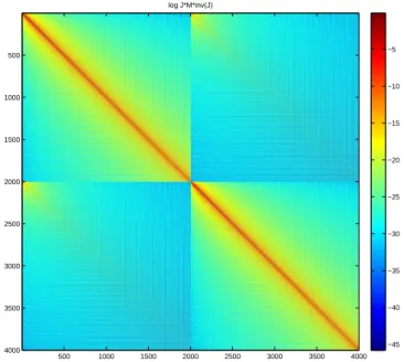
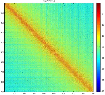
Figure 3 shows the log of JMT,ωJ−1 coefficients and illustrates the
can observe more precisely (51). In particular we can notice that the dis-tribution of the coefficients along the diagonal of the matrix is not regular.
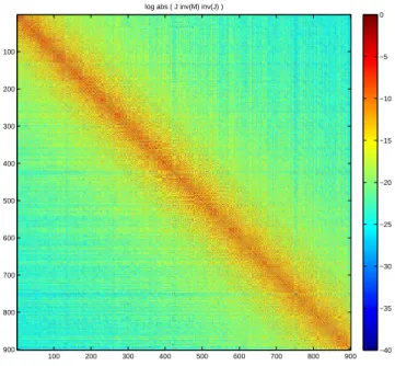
Figure 5 presents the same zoom for JMT,ω−1J−1. This gives an illustration
of the matrix structure of a microlocal operator. Figure 6 represents the
log of JMT,ωJ−1coefficients without smoothing. And finally, figure 7 gives
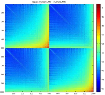
a view of the convergence of our Galerkin approximation, as it presents
the matrix entries of J(Λω− MT,ω−1)J
−1, illustrating lemma 2, its proof,
and lemma 3.
[Figure 3 about here.] [Figure 4 about here.] [Figure 5 about here.] [Figure 6 about here.] [Figure 7 about here.]
2.4
Computation of the discrete control operator
For any real ω, let N (ω) = sup{n, ωn ≤ ω}. Then the dimension of the
vector space L2
ωis equal to N (ω). Let us define the following (φj)1≤j≤2N (ω):
(
φj= ej
ωj for 1 ≤ j ≤ N(ω)
φj= ej−N (ω) for N (ω) + 1 ≤ j ≤ 2N(ω)
(53)
Then (φj)1≤j≤2N (ω) is an orthonormal basis of the Hilbert space Hω =
Πω(H1
0(Ω) ⊕ L2(Ω)).
In this section we compute explicitly`MTφl|φk´H for all 1 ≤ k, l ≤
2N (ω). We recall eisA » ei 0 – = » cos(sωi)ei(x) −ωisin(sωi)ei(x) – eisA » 0 ei – = » sin(sωi)ei(x)/ωi cos(sωi)ei(x) – (54)
We now compute the coefficients of the MT matrix, namely MT n,m =
`MTφn|φm´ H: MT n,m = `MTφn|φm´H = RT 0 `e isABB∗e−isAφn|φm´ Hdt = RT 0 ` „ 0 0 0 χ2 «
e−isAφn|e−isAφm´
Hdt
(55)
or larger than N (ω). For the case (m, n) ≤ N(ω) we have: MT n,m = R0T ` „ 0 0 0 χ2 «
e−isAφn|e−isAφm´
Hds = RT 0 ` „ 0 0 0 χ2 « » cos(sωn)fn(x) ωnsin(sωn)fn(x) – | » cos(sωm)fm(x) ωmsin(sωm)fm(x) – ´ Hds = RT 0 ` » 0 ωnχ2sin(sωn)fn(x) – | » cos(sωn)fm(x) ωmsin(sωm)fm(x) – ´ Hds = RT 0 ((ψ(t)χ0(x)) 2ωnsin(sωn)fn(x)|ωmsin(sωm)fm(x)) L2(Ω)ds = RT 0 ψ 2sin(sωn) sin(sωm) dsR Ωχ 2 0en(x)em(x) dx = an,mGn,m (56) where an,m= Z T 0 ψ2sin(sωm) sin(sωn) ds (57) and Gn,m= Z Ω χ20(x) em(x) en(x) dx (58)
Similarly, for the case n > N (ω), m ≤ N(ω) we have:
MT n,m = RT 0 ` „ 0 0 0 χ2 «
e−isAφn|e−isAφm´
Hds = RT 0 ` „ 0 0 0 χ2 « » sin(sωn)fn(x)/ωn cos(sωn)fn(x) – | » cos(sωm)fm(x) ωmsin(sωm)fm(x) – ´ Hds = RT 0 ` » 0 χ2cos(sωn)fn(x) – | » cos(sωn)fm(x) ωmsin(sωm)fm(x) – ´ Hds = RT 0 (χ 2 cos(sωn)fn(x)|ωmsin(sωm)fm(x))L2(Ω)ds = RT 0 ψ 2cos(sωn) sin(sωm) dsR Ωχ 2 0en(x)em(x) dx = bn,mGn,m (59) where bn,m= Z T 0 ψ2cos(sωn) sin(sωm) ds (60)
For n ≤ N(ω) and m > N(ω) we get:
MT n,m = cn,mGn,m (61) where cn,m= bm,n= Z T 0 ψ2cos(sωm) sin(sωn) ds (62) And for m, n > N (ω): MT n,m = dn,mGn,m (63) where dn,m= Z T 0 ψ2cos(sωm) cos(sωn) ds (64)
The above integrals have to be implemented carefully when |ωn− ωm| is small, even when ψ(t) = 1.
3
Numerical setup and validation
3.1
Geometries and control domains
The code we implemented allows us to choose the two-dimensional domain Ω, as well as the control domain U . In the sequel, we will present some results with three different geometries: square, disc and trapezoid. For each geometry, we have chosen a reference shape of control domain. It consists of the neighborhood of two adjacent sides of the boundary (in the square), of a radius (in the disc), of the base side (in the trapezoid). Then we adjust the width of the control domain, and also its smoothness (see next paragraph). Figures 8, 9 and 10 present these domains, and their respective control domains, either non-smooth (left panels) or smooth (right panels).
[Figure 8 about here.] [Figure 9 about here.] [Figure 10 about here.]
3.2
Time and space smoothing
We will investigate the influence of the regularity of the function χ(t, x) = ψ(t)χ0(x). Different options have been set.
Space-smoothing. The integral (58) defining Gn,m features χ0. In
the literature we find χ0= 1U, so that
Gn,m=
Z
U
en(x) em(x) dx (65)
In [DL09] the authors show that a smooth χ2
0 leads to a more regular
control (see also theorem 3 and lemma 3). Thus for each control domain U we implemented both smooth and non-smooth (constant) cases. The
different implementations of χ0 are:
• constant case: χ0(x, y) = 1U,
• “smooth” case: χ0(x, y) has the same support of U , the width a of the domain {x ∈ Ω, 0 < χ0(x) < 1} is adjustable, and on this domain χ is a polynomial of degree 2. For example, in the square we have: χ0(x, y) = 1Uh1 −“1x≥a+x2 a2.1x<a ” “ 1y≤1−a+(1−y) 2 a2 .1y>1−a ”i (66)
Time-smoothing. Similarly, the time integrals (57,60,62,64) defining a, b, c and d features ψ(t), which is commonly chosen as 1[0,T ]. As pre-viously, better results are expected with a smooth ψ(t). In the code, the integrals (57,60,62,64) are computed explicitly, the different implementa-tions of ψ being:
• constant case ψ = 1[0,T ],
• “smooth case”
ψ(t) =4t(T − t)
T2 1[0,T ] (67)
3.3
Validation of the eigenvalues computation
The code we implemented has a wide range of geometries for Ω. As it is a spectral-Galerkin method, it requires the accurate computation of
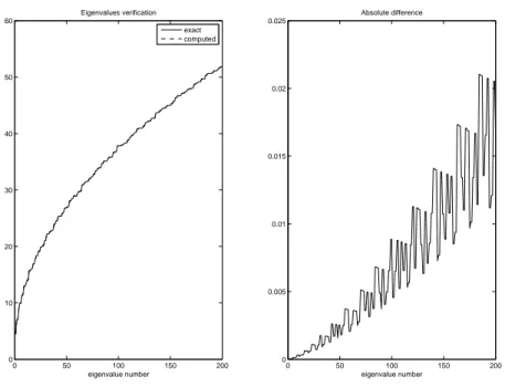
eigenvalues and eigenvectors. We used Matlab eigs1 function. Figure
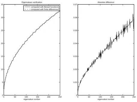
11 shows the comparison between the first 200 exact eigenvalues in the square, and those computed by Matlab with 500 ×500 grid-points. Figure 12 presents the same comparison in the disc, for 250 eigenvalues, the “exact” ones being computed as zeros of Bessel function.
[Figure 11 about here.] [Figure 12 about here.]
3.4
Reconstruction error.
In the sequel, we will denote the input data u = (u0, u1), and its image by the control map w = (w0, w1) = Λ(u0, u1), which will often be called the “control”. We recall from section 2.1 that for a given data u = (u0, u1) to be reconstructed at time T , the optimal control v(t) is given by
v(t) = χ∂te−i(T −t)Aw = χ∂te−i(T −t)AΛ(u) (68)
Then, solving the wave equations (2) forward, with null initial conditions and χv as a forcing source, we reach y = (y0, y1) in time T . Should the
experiment be perfect, we would have (y0, y1) = (u0, u1). The
reconstruc-tion error is then by definireconstruc-tion:
E = v u u t ku0− y0k2 H1(Ω)+ ku1− y1k2L2(Ω) ku0k2 H1(Ω)+ ku1k2L2(Ω) (69)
3.5
Validation for the square geometry
3.5.1 Finite differences versus exact eigenvalues
In this paragraph, we compare various outputs for our spectral method, when the eigenvalues and eigenvectors are computed either with finite-differences or with exact formulas. In this first experiment, we have N × 1www.mathworks.com/access/helpdesk/help/techdoc/ref/eigs.html
N = 500 × 500 grid-points and we use Ne = 100 eigenvalues to compute
the G and MT matrices. The data (u0, u1) is as follows:
u0 = e50
u1 = 0 (70)
Where endenotes the n-th exact eigenvector. The control time T is equal
to 3, the control domain U is 0.2 wide, and we do not use any smoothing. For reconstruction we use 2000 eigenvalues and eigenvectors.
Table 1 shows the condition number of the MT matrices, and
reconstruc-tion errors, which are very similar for both experiments. [Table 1 about here.]
Figure 13 shows the relative reconstruction error between the data u and the reconstructed y for both experiments:
Relative reconstruction error SPn = |U0,n− Y
sp 0,n|
kU0+ U1k
Relative reconstruction error FDn = |U0,n− Y
f d 0,n|
kU0+ U1k
(71)
and similarly for u1 and y1, where U0,nis the n-th spectral coefficient of
the data u0, Y0,nsp is the n-th spectral coefficient (in the basis (φj) defined
by formulas (53) in section 2.4) of the reconstructed y0 when the control
w is obtained thanks to exact eigenvalues and Y0,nf d is the n-th spectral
coefficient of y0when the control w is obtained thanks to finite differences
eigenvalues. The norm kU0+ U1k in our basis (φj) is given by:
kU0+ U1k2=
Ne
X
n=1
U0,n2 + U1,n2 (72)
For exact eigenvalues, we can see that the errors are negligible on the first 100-th spectral coefficients, and quite small on the next ones. We have similar results for finite differences eigenvalues, except that we have an error on the 50-th coefficient. This error does not occur when the reconstruction is done with the same finite differences eigenvectors basis, and it can probably be explained as follows: to compute the reconstructed y from the finite difference control w, we first compute an approximation of w as a function of (x, y) (i.e. on the grid) from its spectral coefficients (on the finite differences eigenvectors basis), then we compute the coefficients of this function on the exact basis (thanks to a very simple integration formula). We thus introduce two sources of errors, projection on the grid and projection on the exact basis, which do not have anything to do with our spectral Galerkin method. Therefore we will not discuss the matter in further detail here.
3.5.2 Impact of the number of eigenvalues
In this paragraph, we still use the same data (70), but the number of
eigen-values and eigenvectors Neused to compute the MT matrices is varying.
Table 2 shows MTcondition numbers and reconstruction errors for various
Newith exact or finite-differences-computed eigenvalues. The
reconstruc-tion is still performed with 2000 exact eigenvalues. We can see that the finite differences eigenvalues lead to almost as good results as exact eigen-values. We also observe in both cases the decrease of the reconstruction error with an increasing number of eigenvalues, as predicted in lemma 3. A 5% error is obtained with 70 eigenvalues (the input data being the 50-th eigenvalue), and 100 eigenvalues lead to less than 2%.
[Table 2 about here.]
4
Numerical experiments
4.1
Frequency localization
In this subsection, the geometry (square) as well as the number of eigen-values used (200 for HUM, 2000 for verification) are fixed. Note also that in this paragraph we use only exact eigenvalues for HUM and verification. The data is also fixed to a given eigenmode, that is:
u0= e50 u1= 0 (73)
where en is the n-th eigenvector of −∆ on the square.
[Figure 14 about here.]
The first output of interest is the spreading of w spectral coefficients, compared to u. Figure 15 shows the spectral coefficients of the input
(u0, u1) and the control (w0, w1) with and without smoothing. As
pre-dicted by theorem 3 and lemma 3 we can see that the main coefficient of (w0, w1) is the 50-th of w0, and also that the smoothing noticeably improves the localization of w.
[Figure 15 about here.]
Similarly we can look at the spectral coefficients of the reconstruction error. Figure 16 presents the reconstruction error (see paragraph 3.4 for a definition) with or without smoothing. We notice that the errors occur
mostly above the cutoff frequency (used for MT,ω computation, and thus
for the control computation). Another important remark should be made here: the smoothing has a spectacular impact on the frequency localiza-tion of the error, as well as on the absolute value of the error (maximum
of 2.10−3without smoothing, and 8.10−7with smoothing), as announced
in theorem 3 and lemma 3.
Remark 1 For other domains, such as the disc and trapezoid, as well as other one-mode input data, we obtain similar results. The results also remain the same if we permute u0 and u1, i.e. if we choose u0 = 0 and u1 equal to one fixed mode.
4.2
Space localization
4.2.1 Dirac experiments
In this section we investigate the localization in space. To do so, we use
“Dirac” functions δ(x,y)=(x0,y0) as data, or more precisely truncations to
a given cutoff frequency of Dirac functions:
u0 = PNi
i=1en(x0, y0) en
u1 = 0 (74)
where Ni is the index corresponding to the chosen cutoff frequency, with
Ni= 100 or 120 in the sequel. Figure 17 shows the data u0and the control
w0 in the square with exact eigenvalues, without smoothing, the results
being similar with smoothing. We can see that the support of w0 is very
similar to u0’s. Figure 18 presents the reconstruction error associated to this experiment. We can see as before that the smoothing produces highly reduced errors.
[Figure 17 about here.] [Figure 18 about here.]
Similarly, we performed experiments with numerical approximation of a Dirac function as input data in the disc and in a trapezoid. Figures
19 and 20 present the space-localization of u0and w0 without smoothing
(we get similar results with smoothing). As previously, the control w0 is
supported by roughly the same area than the input u0. In the disc we can see a small disturbance, located in the symmetric area of the support
of u0with respect to the control domain U . However, this error does not
increase with Ni, as we can see in figure 21 (case Ni= 200) so it remains
compatible with conjecture 1.
Figure 22 shows the reconstruction errors for these experiments, with or without smoothing. As before we notice the high improvement produced by the smoothing. We get similar errors in the trapezoid.
[Figure 19 about here.] [Figure 20 about here.] [Figure 21 about here.] [Figure 22 about here.]
4.2.2 Box experiments in the square
In this paragraph we consider the case u0= 1box, where box = [0.6, 0.8] ×
[0.2, 0.4] is a box in the square. The control domain U is 0.1 wide: U = {x < 0.1 and y > 0.9}. These experiments were performed in the square
with 1000 exact eigenvalues for the MT matrix computation, the input
data u0 being defined thanks to 800 eigenvalues. Figures 23 and 24 show
the space localization of the data u0 and the control w0 without and
with smoothing. As before we can notice that the space localization is
preserved, and that with smoothing the support of w0 is more sharply
defined. Figures 25 and 26 show the reconstruction errors for two different data, the first being the same as in figure 23, and the second being similar but rotated by π/4. We show here only the case with smoothing, the errors being larger but similarly shaped without. We can notice that the errors lows and highs are located on a lattice whose axes are parallel to the box sides. This is compatible with the structure of the wave-front set associated to both input data.
[Figure 23 about here.] [Figure 24 about here.] [Figure 25 about here.] [Figure 26 about here.]
4.3
Reconstruction error
In this section we investigate lemma 3 or more precisely the subsequent remark ??. This remark states that the reconstruction error should de-crease as the inverse of the cutoff frequency without smoothing, and as the inverse of the fifth power of the cutoff frequency with smoothing. To investigate this, we perform a “one-mode” experiment (see paragraph 4.1) using the 50-th mode as input data. We then compute the control with an increasing cutoff frequency, up to 47 (finite differences case) or 82 (exact case), and we compute the reconstruction error, thanks to a larger cutoff frequency (52 in the finite differences case, or 160 in the exact case). Figure 27 represents the reconstruction error (with exact or finite differ-ences eigenvalues) as a function of the cutoff frequency (i.e., the largest eigenvalue used for the control function computation). Figure 28 presents the same results (with finite differences eigenvalues only) for two differ-ent geometries: the square, and the trapezoid (general domain). The log scale allows us to see that the error actually decreases as the inverse of the cutoff frequency without smoothing, and as the inverse of the fifth power of the cutoff frequency with smoothing, according to remark ??.
[Figure 27 about here.] [Figure 28 about here.]
4.4
Energy of the control function
In this paragraph we investigate the impact of the smoothing, the width of the control domain U and the control time T on various outputs such
as the condition number of MT, the reconstruction error ku − yk, and the
norm of the control function kwk.
mode 500) in the square, with exact eigenvalues, 1000 eigenvalues used for computation of MT, 2000 eigenvalues used for reconstruction and ver-ification. We chose various times: 2.5 and 8, plus their “smoothed”
coun-terparts, according to the empirical formula Tsmooth = 15/8 ∗ T . This
increase of Tsmooth is justified on the theoretical level by formulas (31)
and (30) which show that the efficiency of the control is related to a mean value of χ(t, x) on the trajectories. Similarly, we chose various width of U : 1/10 and 3/10, plus their “smoothed” counterpart, which are double. Table 3 presents the numerical results for these experiments. This table draws several remarks. First, the condition number of MT, the recon-struction error and the norm of the control w decrease with increasing time and U . Second, if we compare each non-smooth experiment with its “smoothed” counterpart (the comparison is of course approximate, since the “smoothed” time and width formulas are only reasonable approxima-tions), the condition number seems similar, as well as the norm of the control function w, whereas the reconstruction error is far smaller with smoothing than without.
[Table 3 about here.]
Figures 29 and 30 emphasize the impact of the control time, they present the reconstruction error, the norm of the control, and the condition
num-ber of MT, as a function of the control time (varying between 2.5 and
16), with or without smoothing. Conclusions are similar to the table conclusions.
[Figure 29 about here.] [Figure 30 about here.]
4.5
Condition number
In this section, we investigate conjecture 2. To do so, we compute the condition number of MT,ω, as we have:
cond(MT,ω) = kMT,ωk.kMT,ωk ≃ kMT−1 k.kMT,ωk−1 (75)
Figure 31 shows the condition number of the MT matrix as a function
of the control time or of the last eigenvalue used for the control function computation. According to conjecture 2, we obtain lines of the type
log (cond(MT,ω)) = ω.C(T, U ) (76)
Figure 32 shows for various eigenvalues numbers the following curves:
T 7→log (cond(MT,ω))ω (77)
Similarly, we can draw conclusions compatible with conjecture 2, as these curves seems to converge when the number of eigenvalues grows to infinity.
[Figure 31 about here.] [Figure 32 about here.]
4.6
Non-controlling domains
In this section we investigate two special experiments with non-controlling domains, i.e. such that the geometric control condition is not satisfied whatever the control time.
First we consider the domain presented in Figure 33. [Figure 33 about here.]
For this domain the condition number of the MT matrix is large, and
subsequently we should be experiencing difficulties to reconstruct the data u. We perform one-mode experiments with two different eigenvectors, one being localized in the center of the disc (eigenvalue 60), the other being localized around the boundary (eigenvalue 53) as can be seen on Figure 34.
[Figure 34 about here.]
The various outputs are presented in Table 4, and we can see that the inversion is fairly accurate for the 53rd eigenmode, while it is logically poor for the 60th eigenmode. Moreover, the energy needed for the control process, i.e. the norm of the control w, is small for the 53rd eigenvector, while it is large for the 60-th. We can also notice that the smoothing has the noticeable effect to decrease the reconstruction error, the norm of the control function w being similar.
[Table 4 about here.]
In the second experiment we change the point of view: instead of considering one given domain and two different data, we consider one given data, and two different non-controlling domains. The data is again
u53 (see Figure 34), which is localized at the boundary of the disc. The
first domain is the previous one (see Figure 33), the second domain is presented in Figure 35, it is localized at the center of the disc.
[Figure 35 about here.]
In either case, the condition number of the MT matrix is large, and the
data should prove difficult to reconstruct. Table 5 present the outputs we get for the two domains. As previously, we observe that the control process works fairly well for the appropriate control domain, with a small error as well as a small energy for the control. Conversely, when the control domain does not “see” the input data, the results are poorer: the energy needed is large with or without smoothing, the error is also large without smoothing, it is however small with smoothing.
[Table 5 about here.]
Acknowledgement
The experiments have been realized with Matlab2 software on
Labora-toire Jean-Alexandre Dieudonn´e (Nice) and LaboraLabora-toire Jean Kuntzmann 2The Mathworks, Inc. http://www.mathworks.fr
(Grenoble) computing machines. The INRIA Gforge3has also been used. The authors thank J.-M. Lacroix (Laboratoire J.-A. Dieudonn´e) for his managing of Nice computing machine.
This work has been partially supported by Institut Universitaire de France.
References
[AL98] M. Asch and G. Lebeau. Geometrical aspects of exact
bound-ary controllability of the wave equation. a numerical study. ESAIM:COCV, 3:163–212, 1998.
[BL01] N. Burq and G. Lebeau. Mesures de d´efaut de compacit´e,
ap-plication au syst`eme de lam´e. Ann. Sci. ´Ecole Norm. Sup.,
34(6):817–870, 2001.
[BLR92] C. Bardos, G. Lebeau, and J. Rauch. Sharp sufficient conditions for the observation, control and stabilisation of waves from the boundary. SIAM J.Control Optim., 305:1024–1065, 1992.
[DL09] B. Dehman and G. Lebeau. Analysis of the HUM Control
Oper-ator and Exact Controllability for Semilinear Waves in Uniform Time. to appear in SIAM Control and Optimization, 2009.
[G´er91] P. G´erard. Microlocal defect measures. C.P.D.E, 16:1762–1794,
1991.
[GHL08] R. Glowinski, J. W. He, and J.-L. Lions. Exact and Approximate Controllability for Distributed Parameter Systems: A Numerical Approach. Cambridge University Press, 2008.
[GLL90] R. Glowinski, C.H. Li, and J.L. Lions. A numerical approach to the exact boundary controllability of the wave equation (I). dirichlet controls : description of the numerical methods. Japan J. Appl. Math., 7:1–76, 1990.
[H¨or85] L. H¨ormander. The analysis of linear partial differential
op-erators. III. Grundl. Math. Wiss. Band 274. Springer-Verlag, Berlin, 1985. Pseudodifferential operators.
[Leb92] G. Lebeau. Contrˆole analytique I : Estimations a priori. Duke
Math. J., 68(1):1–30, 1992.
[Lio88] J.-L. Lions. Contrˆolabilit´e exacte, perturbations et
stabilisa-tion de syst`emes distribu´es. Tome 2, volume 9 of Recherches en Math´ematiques Appliqu´ees [Research in Applied Mathematics]. Masson, Paris, 1988.
[MS78] R.-B. Melrose and J. Sjostrand. Singularities of boundary value
problems I. CPAM, 31:593–617, 1978.
[MS82] R.-B. Melrose and J. Sjostrand. Singularities of boundary value
problems II. CPAM, 35:129–168, 1982.
[Rus78] D.-L. Russell. Controllability and stabilizability theory for
lin-ear partial differential equations: recent progress and open ques-tions. SIAM Rev, 20:639–739, 1978.
[Tay81] M. Taylor. Pseudodifferential operators. Princeton University Press, 1981.
[Zua02] E. Zuazua. Controllability of partial differential equations and
its semi-discrete approximations. Discrete and Continuous Dy-namical Systems, 8(2):469–513, 2002.
[Zua05] E. Zuazua. Propagation, observation, and control of waves
ap-proximated by finite difference methods. SIAM Rev, 47(2):197– 243, 2005.
List of Figures
1 Example of optical rays. . . 32 2 Example of optical ray with only transversal reflection
points. . . 33 3 View of the logarithm of the coefficients of the
ma-trix JMTJ− 1
, for the square geometry, with smooth control. This illustrates decay estimates (51) and (52). 34 4 View of the logarithm of the coefficients of the
ma-trix JMTJ− 1
, for the square geometry, with smooth control (zoom). This illustrates decay estimate (51). 35 5 View of the logarithm of the coefficients of the
ma-trix JM−1 T J−
1
, for the square geometry, with smooth control (zoom). . . 36 6 View of the logarithm of the coefficients of the matrix
J MTJ−1, for the square geometry, with non-smooth
control. Note that the color scaling is the same as in Figure 3. . . 37 7 View of the logarithm of the coefficients of the matrix
J£((MT)− 1 )ω− ((MT)ω)− 1 ¤ J−1= J£Λ ω− ((MT)ω)− 1 ¤ J−1,
for the square geometry, with smooth control. The MT matrix is computed with 2000 eigenvalues, the
cutoff frequency ω being associated with the 500th eigenvalue. . . 38 8 Domain and example of a control domain for the square,
with smoothing in space (right panel) or without (left panel). . . 39 9 Domain and example of a control domain for the disc,
with smoothing in space (right panel) or without (left panel). . . 40 10 Domain and example of a control domain for the
trape-zoid, with smoothing in space (right panel) or without (left panel). . . 41 11 Verification of the eigenvalues computation in the square:
exact and finite-differences-computed eigenvalues (left panel), and their absolute difference (right panel). . 42 12 Verification of the eigenvalues computation in the disc:
eigenvalues computed either as zeros of Bessel func-tions or with finite differences (left panel), and their absolute difference (right panel). . . 43
13 Validation experiments in the square: Relative er-rors between the spectral coefficients of the original function u and the reconstructed function y, com-puted with exact eigenvalues (left panels) or finite differences eigenvalues (right panels), for u0 and y0
(top panels) or u1 and y1 (bottom panels). The
er-rors are plotted as a function of the frequency of the eigenvalues. The computation are performed with 100 eigenvalues, corresponding to a frequency of about 38, the reconstruction with 2000, corresponding to a fre-quency of about 160. For the readability of the figure, we plot only the major counterparts of the error, i.e. we stop the plot after frequency 63 (300th eigenvalue). 44 14 Representation on the grid in 3D (left panel) or
con-tour plot (right panel) of the 50-th eigenvector in the square. . . 45 15 One-mode experiment in the square: localization of
the Fourier frequences of (u0, u1) (dashed line) and
(w0, w1) (solid line) for a given time T and a given
do-main U without smoothing (top) and with time- and space-smoothing (bottom). The x-coordinate repre-sents the eigenvalues. The input data u0 is equal to
the 50-th eigenvector, equal to an eigenvalue of about 26.8, and u1= 0. . . 46
16 One-mode experiment in the square: localization of the Fourier coefficients of (u0− y0, u1− y1), where u is
the data and y is the reconstructed function obtained from the control function w, for a given time T and a given domain U without smoothing (top panels) and with time- and space-smoothing (bottom panels). . . 47 17 Space localization of the data u0(top panels) and the
control w0 (bottom panels), for a Dirac experiment
in the square, with exact eigenvalues. These plots correspond to an experiment without smoothing, but it is similar with smoothing. Left panels represent 3D view, and right panels show contour plots. . . 48 18 Difference between the data u0and the reconstructed
function y0 without smoothing (top panels) and with
smoothing (bottom panels) for a dirac experiment in the square, with exact eigenvalues. Left panels repre-sent 3D view, and right panels show contour plots. . 49
19 Space localization of the data u0(top panels) and the
control w0(bottom panels), for a dirac experiment in
the disc. These plots correspond to an experiment without smoothing, but it is similar with smoothing. Left panels represent 3D view, and right panels show contour plots. In this experiment, the input data is defined with Ni= 100 eigenvectors. . . 50
20 Space localization of the data u0(top panels) and the
control w0 (bottom panels), for a dirac experiment
in the trapezoid. These plots correspond to an ex-periment without smoothing, but it is similar with smoothing. Left panels represent 3D view, and right panels show contour plots. In this experiment, the input data is defined with Ni= 120 eigenvectors. . . 51
21 Space localization of the data u0(top panels) and the
control w0(bottom panels), for a dirac experiment in
the disc. These plots correspond to an experiment with smoothing, and it is similar without smoothing. Left panels represent 3D view, and right panels show contour plots. In this experiment, the input data is defined with Ni= 200 eigenvectors. . . 52
22 Difference between the data u0and the reconstructed
function y0 for a dirac experiment in the disc
with-out smoothing (top panels) and with time- and space-smoothing (bottom panels). Left panels represent 3D view, and right panels show contour plots. In this experiment, the input data is defined with Ni = 100
eigenvectors. . . 53 23 Space localization of the control function w0(bottom
panels) with respect to the data u0 (top panels), in
the square, without smoothing: 3D plots on the left, and contour plots on the right. . . 54 24 Space localization of the control function w0(bottom
panels) with respect to the data u0 (top panels), in
the square, with smoothing. Left panels represent 3D view, and right panels show contour plots. . . 55 25 Difference between the data u0and the reconstructed
function y0(top panels) and u1and y1(bottom
pan-els) with smoothing in the square. The data is the identity function of a square whose edges are parallel to the x and y axes. Left panels represent 3D view, and right panels show contour plots. . . 56
26 Difference between the data u0and the reconstructed
function y0(top panels) and u1and y1(bottom
pan-els) with smoothing in the square. The data is the identity function of a square whose edges are parallel to the diagonals of the square. Left panels represent 3D view, and right panels show contour plots. . . 57 27 Reconstruction errors for the finite differences and
ex-act methods, as a function of the cutoff frequency (i.e., the largest eigenvalue used for the control computa-tion), with or without time- and space-smoothing. . 58 28 Reconstruction errors for the finite differences method,
in the square and in the trapezoid, as a function of the cutoff frequency (i.e., the largest eigenvalue used for the control computation), with or without time-and space-smoothing. . . 59 29 Experiments in the square, with exact eigenvalues:
impact of the smoothing on the reconstruction error (top) and on the norm of the control function (bot-tom), as a function of the control time. . . 60 30 Experiments in the square, with exact eigenvalues:
impact of the smoothing on the condition number of the MT matrix, as a function of the control time. . 61
31 Condition number of the MT ,ω matrix as a function
of the cutoff frequency ω for various control times. . 62 32 Ratio of the log of the condition number of the MT ,ω
matrix and the cutoff frequency ω, as a function of the control time for various eigenvalues numbers. . 63 33 Non-controlling domain U without (left) or with (right)
smoothing. This domain consists of the neighborhood of a radius which is truncated around the disc boundary. 64 34 Special modes chosen for experiment with non-controlling
domains, corresponding to the 53rd and 60th eigen-values. . . 65 35 Non-controlling domain U without (left) or with (right)
smoothing. This domain consists of the neighborhood of a radius which is truncated around the disc center. 66
log J*M*inv(J) 500 1000 1500 2000 2500 3000 3500 4000 500 1000 1500 2000 2500 3000 3500 4000 −45 −40 −35 −30 −25 −20 −15 −10 −5
Figure 3: View of the logarithm of the coefficients of the matrix JMTJ− 1
, for the square geometry, with smooth control. This illustrates decay estimates (51) and (52).
log J*M*inv(J) 100 200 300 400 500 600 700 800 900 100 200 300 400 500 600 700 800 900 −40 −35 −30 −25 −20 −15 −10 −5
Figure 4: View of the logarithm of the coefficients of the matrix JMTJ− 1
, for the square geometry, with smooth control (zoom). This illustrates decay estimate (51).
log abs ( J inv(M) inv(J) ) 100 200 300 400 500 600 700 800 900 100 200 300 400 500 600 700 800 900 −40 −35 −30 −25 −20 −15 −10 −5 0
Figure 5: View of the logarithm of the coefficients of the matrix JM−1 T J−
1
, for the square geometry, with smooth control (zoom).
log J*M*inv(J) 500 1000 1500 2000 2500 3000 3500 4000 500 1000 1500 2000 2500 3000 3500 4000 −45 −40 −35 −30 −25 −20 −15 −10 −5 0
Figure 6: View of the logarithm of the coefficients of the matrix JMTJ− 1
, for the square geometry, with non-smooth control. Note that the color scaling is the same as in Figure 3.
log abs (trunc(inv JMJ) − inv(trunc JMJ)) 100 200 300 400 500 600 700 800 900 1000 100 200 300 400 500 600 700 800 900 1000 −50 −45 −40 −35 −30 −25 −20 −15 −10 −5
Figure 7: View of the logarithm of the coefficients of the matrix J£((MT)−
1
)ω− ((MT)ω)− 1
¤ J−1= J£Λω− ((MT)ω)−1¤ J−1, for the square
ge-ometry, with smooth control. The MT matrix is computed with 2000
control domain smooth control domain
Figure 8: Domain and example of a control domain for the square, with smooth-ing in space (right panel) or without (left panel).
control domain smooth control domain
Figure 9: Domain and example of a control domain for the disc, with smoothing in space (right panel) or without (left panel).
control domain smooth control domain
Figure 10: Domain and example of a control domain for the trapezoid, with smoothing in space (right panel) or without (left panel).
0 50 100 150 200 0 10 20 30 40 50 60 eigenvalue number Eigenvalues verification exact computed 0 50 100 150 200 0 0.005 0.01 0.015 0.02 0.025 eigenvalue number Absolute difference
Figure 11: Verification of the eigenvalues computation in the square: exact and finite-differences-computed eigenvalues (left panel), and their absolute difference (right panel).