HAL Id: hal-01871531
https://hal.inria.fr/hal-01871531
Submitted on 11 Sep 2018
HAL is a multi-disciplinary open access
archive for the deposit and dissemination of
sci-entific research documents, whether they are
pub-lished or not. The documents may come from
teaching and research institutions in France or
abroad, or from public or private research centers.
L’archive ouverte pluridisciplinaire HAL, est
destinée au dépôt et à la diffusion de documents
scientifiques de niveau recherche, publiés ou non,
émanant des établissements d’enseignement et de
recherche français ou étrangers, des laboratoires
publics ou privés.
Towards the Verification of Hybrid Co-simulation
Algorithms
Casper Thule, Cláudio Gomes, Julien Deantoni, Peter Larsen, Jörg Brauer,
Hans Vangheluwe
To cite this version:
Casper Thule, Cláudio Gomes, Julien Deantoni, Peter Larsen, Jörg Brauer, et al.. Towards the
Veri-fication of Hybrid Co-simulation Algorithms. Workshop on Formal Co-Simulation of Cyber-Physical
Systems (SEFM satellite), Jun 2018, Toulouse, France. �hal-01871531�
Towards the Verification of
Hybrid Co-simulation Algorithms
?
Casper Thule1( ), Cl´audio Gomes26, Julien Deantoni3, Peter Gorm Larsen1, J¨org Brauer4, and Hans Vangheluwe256
1 Aarhus University, Denmark
{casper.thule,pgl}@eng.au.dk
2 University of Antwerp, Belgium
{claudio.gomes,hans.vangheluwe}@uantwerp.be
3 Polytech Nice Sophia, France
julien.deantoni@polytech.unice.fr
4 Verified Systems International GmbH, Germany
brauer@verified.de
5 McGill University, Canada
6 Flanders Make, Belgium
Abstract. Engineering modern, hybrid systems is becoming increas-ingly difficult due to the heterogeneity between different subsystems. Modelling and simulation techniques have traditionally been used to tackle complexity, but with increasing heterogeneity of the subsystems, it becomes impossible to find appropriate modelling languages and tools to specify and analyse the system as a whole. Co-simulation is a technique to combine multiple models and their simulators in order to analyse the behaviour of the whole system over time. Past research, however, has shown that the na¨ıve combination of simulators can easily lead to in-correct simulation results, especially when co-simulating hybrid systems. This paper shows (i) how co-simulation of a family of hybrid systems can fail to reproduce the order of events that should have occurred (event or-dering); (ii) how to prove that a co-simulation algorithm is correct (w.r.t. event ordering), and if it is incorrect, how to obtain a counterexample showing how the co-simulation fails; and (iii) how to correct an incorrect co-simulation algorithm. We apply the above method to two well known co-simulation algorithms used with the FMI Standard, and we show that one of them is incorrect for the family of hybrid systems under study, under the restrictions of the standard. The conclusion is that either the standard needs to be revised, or one of the algorithms should be avoided. Keywords: hybrid co-simulation, hybrid systems, model checking
?This work was started in the CAMPaM 2017 Workshop, executed under the
frame-work of the COST Action IC1404 – Multi-Paradigm Modelling for Cyber-Physical Systems (MPM4CPS), and partially supported by: Flanders Make vzw, the strate-gic research centre for the manufacturing industry; and PhD fellowship grants from the Agency for Innovation by Science and Technology in Flanders (IWT, dossier 151067).
1
Introduction
Engineered systems are becoming increasingly complex while market pressure shortens the available development time [24]. There are many causes for the increase in complexity, but to a large extent, it is caused by the number of in-teracting subsystems and differences between their domains [31]. Thus, there is a need for an improved development cycle with better tools, techniques, and methodologies [32]. While modelling and simulation have been successfully ap-plied to reduce development costs, these fall short in fostering more integrated development processes [5].
A promising concept for the simulation of systems consisting of coupled com-ponents is collaborative simulation (co-simulation) [23], which is based on the idea that interacting subsystems are best modelled and simulated by dedicated tools and formalisms [33]. Each subsystem is then modelled by a specialised team using mature tools, tailored to the domain of the allocated subsystem. Further, each subsystem internally uses its own simulation engine, so that the most appropriate approximation techniques can be employed. The behaviour of the coupled system is computed by having the simulation tools communicate with one another by exchanging their outputs over time.
In order to run a co-simulation, all that is required is that the participating simulation tools consume the inputs and expose the outputs, of the allocated subsystem, over time. A co-simulation engine then synchronises the interface values of the different subsystems. This powerful approach eases the integration of subsystems simulated by different tools, but also poses some difficulties. In particular, subsystems are modelled and treated as black boxes, and it is dif-ficult in some cases to understand how the coordination of the subsystems—a functionality provided by the co-simulation engine—affects the behaviour of the co-simulated system [19].
One might be tempted to expect that the behaviour computed via co-simulation matches the behaviour of the coupled system. In practice, however, this expecta-tion turns out overly optimistic, and significant deviaexpecta-tions may become visible, which could, for example, be caused by discretization or the timing in which the inputs are set. This is not only due to the inherent limitations of approximate simulations [10], but also due to the internals of the subsystem simulations. It is therefore important to study how a faulty co-simulation can be identified. If a co-simulation preserves specific properties of a system, we then say that the properties of the system are preserved under co-simulation. To serve as a refer-ence for correctness, we consider the properties of the implemented system, i.e. with no co-simulation effects.
This paper contributes to this line of research as follows:
– We identify a novel property called event ordering, which is often implicitly required to be preserved by co-simulations of systems that combine software with physical subsystems.
– We present a characterisation of the event ordering property as a model checking problem [11] based on the Functional Mock-up Interface for co-simulation (FMI) standard [6]. Our method can be utilised to decide whether
a given co-simulation satisfies this property for a restricted class of coupled systems.
– We show how, exemplified using FMI, to adapt the co-simulation master algorithm to preserve the event order, if the property is not preserved. One of the strengths of our approach is that it yields a counterexample when the property is violated. The counter example includes a co-simulation scenario and an execution trace of the co-simulation, which provide valuable insight into how the co-simulation violates the event ordering property. The Maestro [30] master algorithm serves as a case study for our approach.
The remainder of this paper is structured as follows. First, Section 3 presents a primer on co-simulation and co-simulation properties. Afterwards, in Section 4, the event ordering property is demonstrated and described along with an encod-ing of the problem as a model-checkencod-ing instance. Finally, the paper presents a discussion and perspective on future work in Section 5.
2
Background: Co-simulation
Inputs State Outputs extrapolation co-sim step micro-stepFig. 1: Behaviour trace example.
In this section, we present some background concepts in an informal manner. We adopt the definitions and nomenclature introduced in [19] and refer the reader to it for a more rigorous exposition.
A co-simulation is the behaviour trace of a coupled system, produced by the coordination of simulation units. The behaviour trace is a function mapping val-ues to time, representing the outputs generated from each simulation unit and their timestamps. An exam-ple behaviour trace is shown in the bottom of Figure 1. A simulation unit is an executable software entity responsible for simulating a part of the system. To communicate with other simulation units, each sim-ulation unit implements a predefined interface. This allows an orchestrator, described below, to communi-cate with it.
One such communication interface is prescribed by the Functional Mock-up Interface (FMI) standard [6]. A simulation unit implementing the FMI interface is called a Functional Mock-up Unit (FMU). The main functionality of an FMU concerns calculating outputs
based on inputs and time. This is represented in FMI as three C functions: a function to set inputs, a function to perform a step with a given step size, and a function to get outputs.
In the FMI Standard, there is an important restriction [13, p. 104]:
Restriction 1 There is the additional restriction in “slaveInitialized” state that it is not allowed to call fmi2GetXXX functions after fmi2SetXXX functions with-out an fmi2DoStep call in between.
As we show later, this restriction has important consequences on the co-simulation of hybrid systems. Simulation Unit ABS Controller Simulation Unit Car Orchestrator ABS Controller Car
Fig. 2: Co-simulation ar-chitecture.
An orchestrator is a software component that set-s/gets inputs/outputs of each simulation unit, and asks it to estimate the state of its allocated subsys-tem at a future time. For example, in Figure 1, the orchestrator sets an input to the unit at time ti, and asks the unit to compute the state at time ti+ H. The unit in turn might perform multiple micro-steps and employ an input approximation scheme (this is unex-posed to the orchestrator). Then, once the unit is at time ti+ H, the orchestrator requests an output, illus-trated at the bottom of the figure.
The orchestrator follows the co-simulation scenario to know the order in which to ask the simulation unit to simulate and where to copy their outputs. A co-simulation scenario is a de-scription of how the subsystems are interconnected and properties of the co-simulation, e.g. step size. For example, the orchestrator box contains an illustra-tion of how the subsystems are connected, in Figure 2.
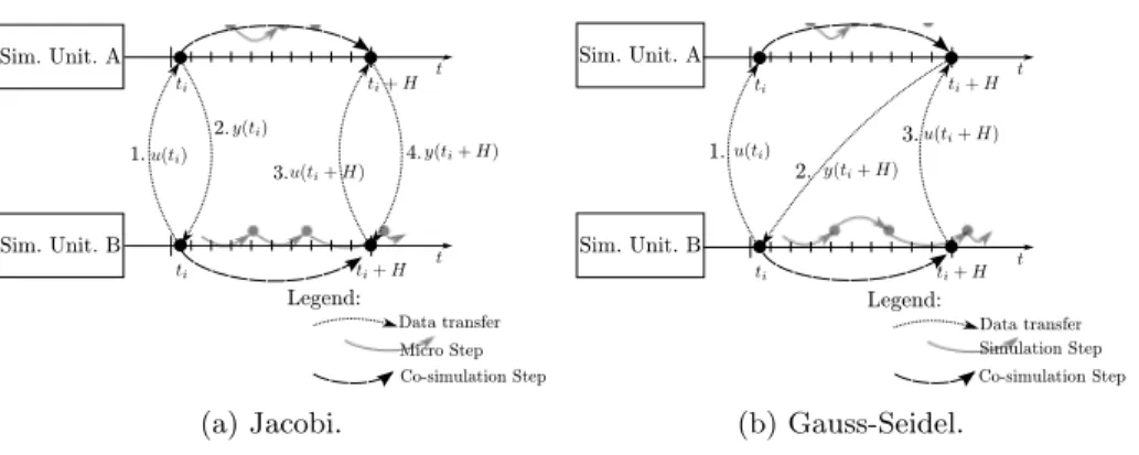
There are three main master algorithms: Jacobi, Gauss-Seidel, and Strong-coupling [25]. We focus on the Jacobi and Gauss-Seidel, illustrated in Figures 3a and 3b. The Jacobi algorithm proceeds by asking all simulators to produce out-puts, then it computes and sets the inputs that all simulators need (illustrated by data transfer arrows in Figure 3a). Afterwards, it asks all simulators to simulate their corresponding subsystem until the next communication time, after which the process repeats. This is represented by simulation step arrows in Figure 3a, where the next communication time is ti+ H.
The Gauss-Seidel algorithm assigns an order to each simulator, and, in that order, computes the inputs of the simulator, then asks the same simulator to simulate to the next time point, obtains its output, and uses that output to compute the input to the next simulator. These steps are repeated until all simulators have simulated until the next time point, and then the process starts over again. See Figure 3b.
3
Related Work: Property Preservation in Co-simulation
In this section, we introduce intuitively the notion of property preservation, and cover examples from the state of the art, where it is studied.
Given a property P that is satisfied by a coupled system, we say that the co-simulation (of the coupled system) preserves P if it also satisfies P. For example, a coupled system representing chemical kinetics always has positive concentrations. Clearly, this property (every concentration variable must be positive) should be preserved in co-simulations.
Legend: Data transfer Micro Step 1. 2. 3. 4. Sim. Unit. A Sim. Unit. B Co-simulation Step (a) Jacobi. Sim. Unit. A Legend: Data transfer Simulation Step 1. 2. 3. Sim. Unit. B Co-simulation Step (b) Gauss-Seidel.
Fig. 3: Coupling algorithms.
In general it is a challenge to ensure that any property of interest is preserved by co-simulations. The following paragraphs provide other examples of property preservation from the state of the art.
Stability. A coupled system is stable when it eventually comes to a rest. Since many systems are engineered to be stable [3], it is important that this property is preserved under co-simulation. The works in [9,28,22,1,17] study the conditions under which the stability property is conserved for selected physical coupled sys-tems. The same works also provide insight into how the co-simulation algorithm can preserve this property.
Energy Conservation. Systems whose models account for the flow of energy fol-low the principle of conservation of energy. That is, no energy is lost when ffol-low- flow-ing between subsystems. This property is not preserved in n¨aive co-simulation algorithms because of the input approximations, and the non-negligible commu-nication step size. The work in [4], extended in [27], demonstrates a co-simulation algorithm that monitors the power flow between simulators and employs a correc-tion scheme to account for the artificial energy introduced by the co-simulacorrec-tion. The work in [26] complements the above work by showing how the energy resid-ual can be used as an error indicator to control the communication step size. Event Synchrony. A co-simulation preserves event synchrony when any event happening at a specific time in the original hybrid system is also reproduced by the co-simulation at the same time. A hybrid system is a system comprising soft-ware and physical subsystems. This is one of the properties studied in [15], in the context of co-simulations involving two simulation units: one responsible for the software subsystem, and the other for a continuous subsystem. In order to en-able an easier comparison of event timestamps, [12] proposes the use of integers, instead of floating point numbers, to represent time. Accurately detecting—and locating the time of—events is paramount to the preservation of the energy and stability properties in a co-simulation. As such, the work in [16] explores how the energy of a hybrid system can be increased when state events are not accurately
reproduced by the co-simulation. It presents a way to find the maximum event detection delay so that the stability is preserved in the co-simulation.
4
Verification of Master Algorithms
The previous section introduced multiple properties that should be preserved in a co-simulation. In particular, it introduced the event synchrony property.
The event synchrony property states that every event happening in a hybrid system, happens at the exact same time in the corresponding co-simulation. An event is a value in the co-simulation whose timestamp should be approximated as closely as possible. For example, the time at which the output of a simulation unit crosses the zero; of the time at which a state machine based FMU changes its output because of a change in its internal discrete state.
In order to detect an event, because its exact time is often difficult to pre-dict without actually asking the units to compute, the master algorithm only detects it after it occurs. Then, to find the exact time of the event, the orches-trator restores the co-simulation to a prior state (where the event has not yet happened) and proceeds with more caution (that is, smaller communication step size). This is repeated until the time of the event is known with sufficiently high accuracy [34]. A consequence is that this property can only be preserved up to some tolerance level, dictated by the precision required for the co-simulation experiment.
4.1 Relaxing Event Synchrony: Event Ordering
The FMI Standard partially supports master algorithms that preserve the event synchrony property. Each FMU is allowed to advance to a time prior to the one requested by the orchestrator, and supports state saving/restoring functional-ities. However, making use of these capabilities in practice may be impossible due to lack of implementation (these are not mandatory), or simply due to the performance degradation entailed by saving/restoring the state multiple times.
As such, the event synchrony property might be too strong. Instead, it might be more useful to require that the sequence of events be preserved, even if the timestamps do not coincide. For example, suppose that the real/correct behaviour of a coupled system, comprised of a software and a physical compo-nent, yields 3 events: (t1, e1), (t2, e2), and (t3, e3), with the timestamps satisfying t1< t2< t3. The co-simulation satisfies the event ordering property if it exhibits the events (t10, e1), (t20, e2), and (t30, e3), with the timestamps satisfying the same order, that is, t10< t20 < t30, but not necessarily equal to t1,t2,t3.
4.2 Problem Formulation
We focus on a restricted class of hybrid systems in order to study an essential challenge related to preserving the event synchrony property. The system under study is illustrated in Figure 4. It consists of a software part, and a physical
part. The software part is represented as a Statechart [20], and the physical part is represented by a differential equation.
Software Physical S0 S1 S2 S3 [after(0.01s)]/e1 [after(0.04s)] [e1]/e2 Legend: Subsystem State [guard]/out-event
Fig. 4: Hybrid systems under study. The software part is
rep-resentative of a control sys-tem that has a timeout mech-anism, triggered whenever the physical part fails to react to some stimuli (an event in this case). The details of the
dy-namics of the physical subsystem are not important. What is important is that its output is a delayed function of the input, so that any change in the input is reflected on the output, e.g., 0.01 seconds later. This is a reasonable abstraction since most physical systems have some sort of inertial reaction to inputs.
An execution of the software subsystem is plotted in Figure 5. At time 0.01s, the event e1 is produced. This event affects the output of the physical system (0.01s later), which is picked up by the software unit, causing it to change to S2 and produce event e2. If the physical plant shows no reaction within 0.04s, then the software will change to state S3.
State
Time (s)
S0 S1 S2 [e1]/e2 [after(0.01s)]/e1Software State
0.02 0 0.01 0.04 0.08 0.1Fig. 5: Sample execution of the system in Figure 4, with Open Modelica [14].
Software FMU u
y
FMU 1 FMU 2 ... FMU N
Fig. 6: Co-Simulation Scenario. For the purposes
of co-simulating the above system using
the FMI Standard,
suppose that the phys-ical subsystem is de-composed into N > 1 FMUs, connected
se-quentially, as shown in Figure 6. The Software FMU implements the simulation of the software subsystem shown in Figure 4. FMU 1 is responsible for the
dy-namics of the physical subsystem in the same figure, which introduces a 0.01s delay between input and output. The remaining FMUs are identity functions and will be referred to as propagate FMUs. All the FMUs here behave according to the FMI Standard 2.0, respecting Restriction 1. That is, no event is detected when a new input is set.
Using the Jacobi algorithm to co-simulate the scenario in Figure 6, with N= 3 and co-simulation step size H = 0.01, leads to the software execution trace depicted in Figure 7. The events produced in this trace are the same as the ones in the correct execution in Figure 5, but their timestamps are different. Event e1 is produced at time 0.02s instead of 0.01s, and the reaction of the physical subsystem is detected later at time 0.06s, instead of 0.02s.
State Time (s) S0 S1 S2 Software State 0.02 0 0.01 0.04 0.08 0.1 [e1]/e2 [after(0.01s)]/e1 0.06
Fig. 7: Co-simulation using the Jacobi algorithm of the scenario in Figure 6. Parameters: N = 3, H = 0.01. Produced with Maestro from INTO-CPS [30].
Naturally, the smaller the communication step size H, the smaller the delay introduced by the propagate FMUs.
What this example illustrates is that, due to Restriction 1, the size of the co-simulation scenario also plays a role in the delay introduced. By adding more propagate FMUs to the example scenario, we get a qualitatively different event sequence, as shown in Figure 8, where the final state of the software subsystem is S3, instead of S2. The excessive delay, accidentally introduced by the Jacobi algorithm, causes the software timeout to be triggered.
In general one would like to have co-simulations that either do not introduce artificial delays, or that, at least, introduce a delays that depend only on the communication step size, so that it is easier to satisfy the event ordering prop-erty. In the following subsections we use model checking to formally study the ordering of this property for the hybrid system shown in Figure 4, with a variable structure co-simulation scenario illustrated in Figure 6. In the experiments the co-simulation step size is kept the same, although it is straightforward to take its variation into account.
State S1 S2 Time (s) Software State 0.02 0 0.01 0.04 0.06 0.08 0.1 [after(0.01s)]/e1 [after(0.04s)] S3 S0
Fig. 8: Co-simulation using the Jacobi algorithm of the scenario in Figure 6. Parameters: N = 6, H = 0.01. Produced with Maestro from INTO-CPS [30].
4.3 Model Checking the Jacobi Algorithm
We use the ProMeLa [21] notation to model the FMUs, and the master algorithm. The Promela language uses a textual syntax to describe parallel and sequential processes, communication channels, and non-determinism.
Listing 1.1: Channels
1 mtype:events = {e0, e1};
2 typedef channels {
3 chan in = [0] of {mtype:events}; 4 chan out = [0] of {mtype:events}; 5 chan step = [0] of {int}; 6 }
The Promela model follows closely the co-simulation scenario sketched in Figure 6. The communication between the master algorithm and the FMUs is made via three channels: one to set inputs, one to set outputs, and one to perform a co-simulation step. These channels are detailed in Listing 1.1. The in and step channels are read by the FMU, while the out channel is read by the master algorithm.
Listing 1.2: Statechart FMU
1 proctype stateFMU(channels chans) {
2 int t_time = 0;
3 mtype:events input;
4 do
5 :: chans.step ? t_time -> 6 if
7 /* if state is 0 and more than 1 time unit have passed, then change the state
,→ to 1 and output an event. */ 8 :: (state == 0) ->
9 if
10 :: (t_time > 1) -> 11 state=1;
12 chans.out ! e1; /* e1 is the output that we are interested in receiving
13 :: else -> chans.out ! e0; 14 fi;
15 /* If the state is 1 and 4 additional time units have passed, then change to
,→ state 3 */ 16 :: (state == 1) -> 17 if
18 :: t_time > 5 & input != e1 -> state = 3; 19 :: input == e1 -> state = 2;
20 :: else -> skip; 21 fi;
22 chans.out ! e0;
23 :: (state == 2) -> chans.out ! e1; 24 :: else -> chans.out ! e0; 25 fi;
26 :: chans.in ? input
27 :: (terminate == 1) -> break; 28 od;
29 }
The FMU corresponding to the software subsystem is modelled in ProMeLa by implementing the reaction to events received from the channels in and step. When a event is present in channel in, it is stored in the intermediate variable input, such that it can be accessed when an event is present in channel step. When an event is present in channel step, the FMU follows the state machine of the software subsystem, taking into account that the time is represented as an integer and the communication step size is 0.01s. Listing 1.2 presents this model. The other FMUs are propagate FMUs. As such, the FMU model shown in Listing 1.3 just stores and outputs whatever input it receives.
Listing 1.3: Propagate FMU
1 proctype propFMU(channels chans){
2 mtype:events inp;
3 int t_time = 0; 4 do
5 :: chans.in ? inp
6 :: chans.step ? t_time -> chans.out ! inp; 7 :: (terminate == 1) -> break;
8 od; 9 }
The Jacobi master algorithm essentially sends events through the in chan-nel of each FMU, asks the FMU to step via the step chanchan-nel, and stores the output events at the out channels. The non-deterministic aspect of this model is encoded in the choice of the number of propagate FMUs that can be added to the scenario. The number of FMUs (maxN) is limited to 10, as it is enough to prove this property. The implementation is shown in Listing 1.4.
Listing 1.4: The Jacobi Master Algorithm in ProMeLa
1 proctype MAJacobi(){
2 int propagateCount;
3 select ( propagateCount : 1 .. (maxN-1) ); 4 int FMUCount = propagateCount + 1;
5
6 channels fmuChannels[maxN];
7 mtype:events inputs[maxN];
8
9 smpid = run stateFMU(fmuChannels[0]); 10
11 int i; 12 for(i : 1 .. propagateCount){ 13 run propFMU(fmuChannels[i]); 14 } 15 16 do 17 :: time < endTime -> 18 /* Step the FMUs */ 19 for(i : 0 .. FMUCount-1){ 20 fmuChannels[i].step ! time+1; 21 }
22
23 /* Retrieve the outputs */ 24 for(i : 0 .. FMUCount-1){
25 fmuChannels[i].out ? inputs[(i + 1) % (FMUCount)]; 26 } 27 28 /* Set inputs */ 29 for(i : 0 .. FMUCount-1){ 30 fmuChannels[i].in ! inputs[i] 31 } 32 33 time++; 34 :: else -> 35 terminate = 1; 36 break; 37 od; 38 }
The event ordering property can be encoded in this model as a reachability property: the Statechart FMU eventually reaches S2. This is shown in Listing 1.5. The state variable is global, and is set as part of the execution of the FMU.
Listing 1.5: Eventually Correct LTL formula.
1 ltl eventuallyCorrect { <> (state == 2)}
Using SPIN [21] to carry out the verification of this property, applied to Listing 1.4, quickly shows that it cannot be verified. The error trail provides a counter example execution, by showing that S3 is reached when there are four propagate FMUs. Informally, the error trail is the following: At step 2 (0.02 s), e1 is outputted from the Statechart FMU. At step 3 (0.03 s) it is outputted from the following propagate FMU. At step 4 it is outputted from the second propagate FMU, at step 5 it is outputted from the third propagate FMU. Finally, at step 6 it is outputted from the last propagate FMU but this is the same time as the Software FMU transitions to S3. Therefore, the Statechart FMU never reaches S2. This is consistent with the result in Figure 8.
4.4 Model Checking the Gauss-Seidel Algorithm
The Gauss-seidel algorithm is introduced in Section 2 and illustrated in Fig-ure 3b. The main difference between this algorithm and the Jacobi is in the timestamp of the outputs and inputs provided to the simulation units. From the perspective of a simulation unit, the Gauss-Seidel algorithm provides future inputs to the unit, before asking it to compute a co-simulation step. This allows the unit to react to the inputs without any delay [18]. Its implementation is detailed in Listing 1.6.
Listing 1.6: The Gauss-Seidel Master Algorithm in ProMeLa
1 proctype MAGauss(){
2 int propagateCount;
3 select ( propagateCount : 1 .. (maxN-1) ); 4 int FMUCount = propagateCount + 1;
5
6 channels fmuChannels[maxN];
7 mtype:events inputs[maxN];
8 9 run stateFMU(fmuChannels[0]); 10 11 int i; 12 for(i : 1 .. FMUCount-1){ 13 run propFMU(fmuChannels[i]); 14 } 15 16 do 17 :: time < endTime -> 18 for(i : 0 .. FMUCount-1){ 19 /* Step the FMU */
20 fmuChannels[i].step ! time + 1; 21
22 /* Retrieve the output */
23 fmuChannels[i].out ? inputs[(i + 1) % FMUCount]; 24
25 /* Set the input */
26 fmuChannels[(i + 1) % FMUCount].in ! inputs[(i + 1) % FMUCount] 27 } 28 time++; 29 :: else -> 30 terminate = 1; 31 break; 32 od; 33 }
Verifying Listing 1.6 with the LTL formula in Listing 1.5 shows that the Gauss-seidel algorithm correctly preserves the execution sequence of the events. This matches our intuition since the Gauss-Seidel algorithm allows each FMU to perform computation while knowing the future input. Therefore, Restriction 1 does not affect the ability to propagate events instantaneously. The next section discusses these results.
5
Discussion and Future Work
In this paper we have shown how a co-simulation using the Jacobi algorithm, and respecting the FMI Standard, can fail to preserve the event ordering property. To this end, we picked a particular class of hybrid systems that are sensitive to delays.
The correctness property we used is a weak form of event synchrony: the order of events is preserved, but their timestamps can be different than the ones happening in the correct behaviour of the coupled system. Under the restrictions of the FMI Standard, two master algorithms have been used to study the prop-erty: The Jacobi and the Gauss-Seidel. It is shown that the Jacobi algorithm does not preserve it, in general making it unsuitable for general, hybrid FMI based co-simulation.
Albeit a very simple example, the hybrid system used is meant to illus-trate that, based on minimum information on the FMUs, we can prove if a co-simulation algorithm is appropriate or not for a scenario. The proof is based on an abstraction of the FMU in the form of timed automata and the definition of properties to be respected by some FMUs. To extend this preliminary work, we intend to explore how to deal with black box simulation units, so that a conservative (and provably correct) abstraction can be built for them. It is also important for an FMU to expose some of the properties that must be preserved without revealing the internal details, keeping intellectual property safe.
To illustrate, in the previous example, if we expose the shortest timed reaction of each software FMU, and the input-to-output propagation time of each FMU then we can determine which communication step size can be used in order to ensure the order of the event sequence with the Jacobi algorithm. To see how the step size H can be computed, let T denote the smallest timeout used in the software FMU, and P(H) denote the largest propagation time from any output to itself, for the communication step size H. For the scenario in Figure 6, P(H) = H × (N + 1). Then the communication step size must be chosen so that P(H) < T .
This example shows that the Jacobi algorithm is still suitable for black box co-simulations, since exposing the shortest timed reaction and the propagation time does not expose the Intellectual Property of the subsystems.
Providing abstract information from the FMU is common in research on black box co-simulation (e.g., exposing the Jacobian [29], exposing the I/O feedthrough [2], exposing the maximum allowed step size [7]). While this is usually carried out to allow the setup of a co-simulation algorithm, we propose here to expose the minimum, relevant information to have a correct co-simulation, ie. to allow verification such as model checking of the co-simulation.
The FMI webpage7contains a list of tools capable of performing co-simulation, and in order to be on this list, a tool must pass some tests. These tests, however, are limited – for example they only concern simulation of a single FMU, and not an actual co-simulation. In the long term, this research aims at producing a set of benchmarks, for various correctness properties, that can be used by the research community in the development of co-simulation tools. This idea is inspired by the work of [8], which defined the building blocks of these benchmarks.
References
1. Arnold, M.: Stability of Sequential Modular Time Integration Methods for Coupled Multibody System Models. Journal of Computational and Nonlinear Dynamics 5(3), 9 (may 2010)
2. Arnold, M., Clauß, C., Schierz, T.: Error Analysis and Error Estimates for
Co-simulation in FMI for Model Exchange and Co-Simulation v2.0. In: Sch¨ops, S.,
Bar-tel, A., G¨unther, M., ter Maten, W.E.J., M¨uller, C.P. (eds.) Progress in Differential-Algebraic Equations. pp. 107–125. Springer Berlin Heidelberg, Berlin, Heidelberg (2014)
3. Astr¨om, K.J., Wittenmark, B.: Computer-controlled systems: theory and design. Courier Corporation (2011)
4. Benedikt, M., Watzenig, D., Zehetner, J., Hofer, A.: NEPCE-A Nearly Energy Preserving Coupling Element for Weak-coupled Problems and Co-simulation. In: IV International Conference on Computational Methods for Coupled Problems in Science and Engineering, Coupled Problems. pp. 1–12. Ibiza, Spain (jun 2013) 5. Blochwitz, T., Otter, M., Arnold, M., Bausch, C., Clauss, C., Elmqvist, H.,
Jung-hanns, A., Mauss, J., Monteiro, M., Neidhold, T., Neumerkel, D., Olsson, H., Peetz, J.V., Wolf, S.: The Functional Mockup Interface for Tool independent Exchange of Simulation Models. In: 8th International Modelica Conference. pp. 105–114.
Link¨oping University Electronic Press; Link¨opings universitet, Dresden, Germany
(jun 2011)
6. Blockwitz, T., Otter, M., Akesson, J., Arnold, M., Clauss, C., Elmqvist, H., Friedrich, M., Junghanns, A., Mauss, J., Neumerkel, D., Olsson, H., Viel, A.: Func-tional Mockup Interface 2.0: The Standard for Tool independent Exchange of
Sim-ulation Models. In: 9th International Modelica Conference. pp. 173–184. Link¨oping
University Electronic Press, Munich, Germany (nov 2012)
7. Broman, D., Brooks, C., Greenberg, L., Lee, E.A., Masin, M., Tripakis, S., Wet-ter, M.: Determinate composition of FMUs for co-simulation. In: Eleventh ACM International Conference on Embedded Software. p. Article No. 2. IEEE Press Piscataway, NJ, USA, Montreal, Quebec, Canada (2013)
8. Broman, D., Greenberg, L., Lee, E.A., Masin, M., Tripakis, S., Wetter, M.: Re-quirements for Hybrid Cosimulation Standards. In: 18th International Conference on Hybrid Systems: Computation and Control. pp. 179–188. HSCC ’15, ACM New York, NY, USA, Seattle, Washington (2015)
9. Busch, M.: Continuous approximation techniques for co-simulation methods: Anal-ysis of numerical stability and local error. ZAMM - Journal of Applied Mathematics and Mechanics 96(9), 1061–1081 (sep 2016)
10. Cellier, F.E., Kofman, E.: Continuous System Simulation. Springer Science & Busi-ness Media (2006)
11. Clarke, E.M., Veith, H.: In: Verification: Theory and Practice, Essays Dedicated to Zohar Manna on the Occasion of His 64th Birthday. Lecture Notes in Computer Science, vol. 2772, pp. 208–224. Springer (2003)
12. Cremona, F., Lohstroh, M., Broman, D., Lee, E.A., Masin, M., Tripakis, S.: Hybrid co-simulation: it’s about time. Software & Systems Modeling (nov 2017)
13. FMI: Functional Mock-up Interface for Model Exchange and Co-Simulation. Tech. rep. (2014)
14. Fritzson, P., Aronsson, P., Pop, A., Lundvall, H., Nystrom, K., Saldamli, L., Bro-man, D., Sandholm, A.: Openmodelica - a free open-source environment for system modeling, simulation, and teaching. In: 2006 IEEE Conference on Computer Aided Control System Design, 2006 IEEE International Conference on Control Applica-tions, 2006 IEEE International Symposium on Intelligent Control. pp. 1588–1595 (Oct 2006)
15. Gheorghe, L., Bouchhima, F., Nicolescu, G., Boucheneb, H.: A Formalization of Global Simulation Models for Continuous/Discrete Systems. In: Summer Computer Simulation Conference. pp. 559–566. SCSC ’07, Society for Computer Simulation International San Diego, CA, USA, San Diego, CA, USA (jul 2007)
16. Gomes, C., Karalis, P., Navarro-L´opez, E.M., Vangheluwe, H.: Approximated
Sta-bility Analysis of Bi-modal Hybrid Co-simulation Scenarios. In: 1st Workshop on Formal Co-Simulation of Cyber-Physical Systems. pp. 345–360. Springer, Cham, Trento, Italy (2017)
17. Gomes, C., Legat, B., Jungers, R.M., Vangheluwe, H.: Stable Adaptive simulation : A Switched Systems Approach. In: IUTAM Symposium on Co-Simulation and Solver Coupling. p. to appear. No. 1, Darmstadt, Germany (2017) 18. Gomes, C., Meyers, B., Denil, J., Thule, C., Lausdahl, K., Vangheluwe, H., De Meulenaere, P.: Semantic Adaptation for FMI Co-simulation with Hierarchical Simulators. SIMULATION pp. 1—-29 (2018)
19. Gomes, C., Thule, C., Broman, D., Larsen, P.G., Vangheluwe, H.: Co-simulation: a Survey. ACM Computing Surveys 51(3), Article 49 (apr 2018)
20. Harel, D.: Statecharts: a visual formalism for complex systems. Science of Com-puter Programming 8(3), 231–274 (jun 1987)
21. Holzmann, G.: The model checker SPIN. IEEE Transactions on Software Engineer-ing 23(5), 279–295 (may 1997)
22. Kalmar-Nagy, T., Stanciulescu, I.: Can complex systems really be simulated? Ap-plied Mathematics and Computation 227, 199–211 (jan 2014)
23. K¨ubler, R., Schiehlen, W.: Modular Simulation in Multibody System Dynamics.
Multibody System Dynamics 4(2-3), 107–127 (aug 2000)
24. Lee, E.A.: Cyber Physical Systems: Design Challenges. In: 11th IEEE International Symposium on Object Oriented Real-Time Distributed Computing (ISORC). pp. 363–369 (2008)
25. Palensky, P., Van Der Meer, A.A., Lopez, C.D., Joseph, A., Pan, K.: Cosimulation of Intelligent Power Systems: Fundamentals, Software Architecture, Numerics, and Coupling. IEEE Industrial Electronics Magazine 11(1), 34–50 (mar 2017)
26. Sadjina, S., Kyllingstad, L.T., Skjong, S., Pedersen, E.: Energy conservation and power bonds in co-simulations: non-iterative adaptive step size control and error estimation. Engineering with Computers 33(3), 607–620 (jul 2017)
27. Sadjina, S., Pedersen, E.: Energy Conservation and Coupling Error Reduction in
Non-Iterative Co-Simulations. Tech. rep. (jun 2016),http://arxiv.org/abs/
1606.05168
28. Schweizer, B., Li, P., Lu, D.: Explicit and Implicit Cosimulation Methods: Stability and Convergence Analysis for Different Solver Coupling Approaches. Journal of Computational and Nonlinear Dynamics 10(5), 051007 (sep 2015)
29. Sicklinger, S., Belsky, V., Engelmann, B., Elmqvist, H., Olsson, H., W¨uchner, R.,
Bletzinger, K.U.: Interface Jacobian-based Co-Simulation. International Journal for Numerical Methods in Engineering 98(6), 418–444 (may 2014)
30. Thule, C., Lausdahl, K., Larsen, P.G., Meisl, G.: Maestro: The into-cps co-simulation orchestration engine (2018), submitted to Simulation Modelling Practice and Theory
31. Tomiyama, T., D’Amelio, V., Urbanic, J., ElMaraghy, W.: Complexity of Multi-Disciplinary Design. CIRP Annals - Manufacturing Technology 56(1), 185–188 (2007)
32. Van der Auweraer, H., Anthonis, J., De Bruyne, S., Leuridan, J.: Virtual engineer-ing at work: the challenges for designengineer-ing mechatronic products. Engineerengineer-ing with Computers 29(3), 389–408 (2013)
33. Vangheluwe, H., De Lara, J., Mosterman, P.J.: An introduction to multi-paradigm modelling and simulation. In: AI, Simulation and Planning in High Autonomy Systems. pp. 9–20. SCS (2002)
34. Zhang, F., Yeddanapudi, M., Mosterman, P.J.: Zero-Crossing Location and Detec-tion Algorithms For Hybrid System SimulaDetec-tion. In: IFAC Proceedings Volumes. vol. 41, pp. 7967–7972. Elsevier Ltd, Seoul, Korea (jul 2008)