HAL Id: hal-02141469
https://hal.archives-ouvertes.fr/hal-02141469
Submitted on 27 May 2019
HAL is a multi-disciplinary open access
archive for the deposit and dissemination of
sci-entific research documents, whether they are
pub-lished or not. The documents may come from
teaching and research institutions in France or
abroad, or from public or private research centers.
L’archive ouverte pluridisciplinaire HAL, est
destinée au dépôt et à la diffusion de documents
scientifiques de niveau recherche, publiés ou non,
émanant des établissements d’enseignement et de
recherche français ou étrangers, des laboratoires
publics ou privés.
Combining Voxel and Normal Predictions for
Multi-View 3D Sketching
Johanna Delanoy, David Coeurjolly, Jacques-Olivier Lachaud, Adrien
Bousseau
To cite this version:
Johanna Delanoy, David Coeurjolly, Jacques-Olivier Lachaud, Adrien Bousseau. Combining Voxel
and Normal Predictions for Multi-View 3D Sketching. Computers and Graphics, Elsevier, 2019,
Proceedings of Shape Modeling International 2019, 82, pp.65–72. �10.1016/j.cag.2019.05.024�.
�hal-02141469�
Combining Voxel and Normal Predictions for Multi-View 3D Sketching
Johanna Delanoya, David Coeurjollyb, Jacques-Olivier Lachaudc, Adrien Bousseaud
aInria, Universit´e Cˆote d’Azur bUniversit´e de Lyon, CNRS, LIRIS
cLaboratoire de Math´ematiques (LAMA), UMR 5127 CNRS, Universit´e Savoie Mont Blanc dInria, Universit´e Cˆote d’Azur
Abstract
Recent works on data-driven sketch-based modeling use either voxel grids or normal/depth maps as geometric representations com-patible with convolutional neural networks. While voxel grids can represent complete objects – including parts not visible in the sketches – their memory consumption restricts them to low-resolution predictions. In contrast, a single normal or depth map can capture fine details, but multiple maps from different viewpoints need to be predicted and fused to produce a closed surface. We propose to combine these two representations to address their respective shortcomings in the context of a multi-view sketch-based modeling system. Our method predicts a voxel grid common to all the input sketches, along with one normal map per sketch. We then use the voxel grid as a support for normal map fusion by optimizing its extracted surface such that it is consistent with the re-projected normals, while being as piecewise-smooth as possible overall. We compare our method with a recent voxel prediction system, demonstrating improved recovery of sharp features over a variety of man-made objects.
Keywords: Sketch-Based Modeling, Deep Learning, Surface Regularization, Voxels, Normal Map
1. Introduction
1
As many related fields, sketch-based modeling recently
wit-2
nessed major progress thanks to deep learning. In particular,
3
several authors demonstrated that generative convolutional
net-4
works can predict 3D shapes from one or several line drawings
5
[1, 2, 3, 4]. A common challenge faced by these methods is the
6
choice of a geometric representation that can both represent the
7
important features of the shape while also being compatible with
8
convolutional neural networks. Voxel grids form a natural 3D
ex-9
tension to images, and were used by Delanoy et al. [1] to predict
10
a complete object from as little as one input drawing. This
com-11
plete prediction allows users to rotate around the 3D shape before
12
creating drawings from other viewpoints. However, the memory
13
consumption of voxel grids limits their resolution, resulting in
14
smooth surfaces that lack details. Alternatively, several methods
15
adopt image-based representations, predicting depth and normal
16
maps from one or several drawings [2, 3, 4]. While these maps
17
can represent finer details than voxel grids, each map only shows
18
part of the surface, and multiple maps from different viewpoints
19
need to be fused to produce a closed object.
20
Motivated by the complementary strengths of voxel grids and
21
normal maps, we propose to combine both representations within
22
the same system. Our approach builds on the voxel prediction
23
network of Delanoy et al. [1], which produces a volumetric
pre-24
diction of a shape from one or several sketches. We complement
25
this architecture with a normal prediction network similar to the
26
one used by Su et al. [4], which we use to obtain a normal map for 27
each input sketch. The voxel grid thus provides us with a com- 28
plete, closed surface, while the normal maps allow us to recover 29
details in the parts seen from the sketches. 30
Our originality is to not only use the voxel grid as a prelim- 31
inary prediction to be shown to the user, but also as a support 32
for normal map fusion. To do so, we first locate the voxels de- 33
lineating the object’s boundary, and re-project the normal maps 34
on the resulting surface to obtain a distribution of candidate nor- 35
mals for each surface element. We then solve for the smoothest 36
normal field that best agrees with these observations [5]. Finally, 37
we optimize the surface elements to best align with this normal 38
field [6]. We evaluate our approach on the dataset of Delanoy 39
et al. [1], on which we recover smoother surfaces with sharper 40
discontinuities. 41
2. Related work 42
Reconstructing 3D shapes from line drawings has a long his- 43
tory in computer vision and computer graphics. A number of 44
methods tackle this problem by geometric means, for instance by 45
detecting and enforcing 3D relationships between lines, like par- 46
allelism and orthogonality [7, 8, 9, 10, 11]. However, computing 47
these geometric constraints often require access to a clean, well- 48
structured representation of the drawing, for instance in the form 49
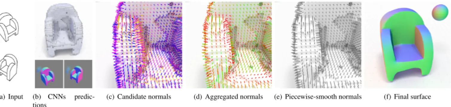
(a) Input (b) CNNs predic-tions
(c) Candidate normals (d) Aggregated normals (e) Piecewise-smooth normals (f) Final surface
Figure 1: Overview of our method. Our method takes as input multiple sketches of an object (a). We first apply existing deep neural networks to predict a volumetric reconstruction of the shape as well as one normal map per sketch (b). We re-project the normal maps on the voxel grid (c, blue needles for the first normal map, yellow needles for the second normal map), which complement the surface normal computed from the volumetric prediction (c, pink needles). We aggregate these different normals into a distribution represented by a mean vector and a standard deviation (d, colors denote low variance in green and high variance in red). We optimize this normal field to make it piecewise smooth (e) and use it to regularize the surface (f). The final surface preserves the overall shape of the predicted voxel grid as well as the sharp features of the predicted normal maps.
often require user annotations to disambiguate multiple
interpre-1
tations, or to deal with missing information.
2
Data-driven methods hold the promise to lift the above
limi-3
tations by providing strong priors on the shapes that a drawing
4
can represent. In particular, recent work exploit deep neural
net-5
works to predict 3D information from as little as a single bitmap
6
line drawing. However, convolutional neural networks have been
7
originally developed to work on images, and several alternative
8
solutions have been proposed to adapt such architectures to
pro-9
duce 3D shapes.
10
A first family of methods focuses on parametric shapes such as
11
buildings [12], trees [13], and faces [14], and train deep networks
12
to regress their parameters. While these methods produce 3D
13
shapes of very high quality, extending them to new classes of
14
objects require designing novel parametric models by hand.
15
A second family of methods target arbitrary shapes and rely on
16
encoder-decoder networks to convert the input drawing into 3D
17
representations. Among them, Delanoy et al. [1] rely on a voxel
18
grid to represent a complete object. Users of their system can thus
19
visualize the 3D shape, including its hidden parts, as soon as they
20
have completed a single drawing. Their system also supports
ad-21
ditional drawings created from different viewpoints, which allow
22
the network to refine its prediction. Nevertheless, their system
23
is limited to voxel grids of resolution 643, which is too little to
24
accurately capture sharp features. Alternatively, Su et al. [4] and
25
Li et al. [3] propose encoder-decoder networks to predict normal
26
and depth maps respectively. While these maps only represent
27
the geometry visible in the input drawing, Li et al. allow users
28
to draw the object from several viewpoints and fuse the
result-29
ing depth maps to obtain a complete object. A similar
image-30
based representation has been proposed by Lun et al. [2], who
31
designed a deep network to predict depth maps from 16
view-32
points, given one to three drawings as input. In both cases,
fus-33
ing the multiple depth maps requires careful point set registration
34
and optimization to compensate for misalignment. Our approach
35
combines the strength of both voxel-based and image-based rep- 36
resentations. On the one hand, per-sketch normal maps provide 37
high-resolution details about the shape, while on the other hand, 38
the voxel grid provides an estimate of the complete shape as well 39
as a support surface for normal fusion. By casting normal fusion 40
as the reconstruction of a piecewise-smooth normal field over the 41
voxel surface, our method alleviates the need for precise align- 42
ment of the normal maps. 43
Line drawing interpretation is related to the problem of 3D 44
reconstruction from photographs, for which numerous deep- 45
learning solutions have been proposed by the computer vision 46
community. While many approaches rely on voxel-based [15, 16] 47
and image-based [17] representations as discussed above, other 48
representations have been proposed to achieve finer reconstruc- 49
tions. Octrees have long been used to efficiently represent volu- 50
metric data, although their implementation in convolutional net- 51
works requires the definition of custom operations, such as con- 52
volutions on hash tables [18] or cropping of octants [19]. Point 53
sets have also been considered as an alternative to voxel-based 54
or image-based representations [20], and can be converted to 55
surfaces in a post-process as done for depth map fusion. More 56
recently, several methods attempted to directly predict surfaces. 57
Pixel2Mesh [21] relies on graph convolutional networks [22] to 58
predict deformations of a template mesh. However, this approach 59
is limited to shapes that share the same topology as the tem- 60
plate, an ellipsoid in their experiments. In contrast, Groueix et 61
al. [23] can handle arbitrary topology by predicting multiple sur- 62
face patches that cover the shape. Since these patches do not form 63
a single, closed surface, their approach can also be used to gen- 64
erate a dense point set from which a surface can be computed as 65
a post-process. In contrast to the above approaches, we chose to 66
combine voxel-based and image-based representations because 67
both can be implemented using standard convolutional networks 68
on regular grids. 69
3. Overview
1
Our method takes as input several sketches of a shape drawn
2
from different known viewpoints (Figure 1a). We first use
ex-3
isting deep neural networks [1, 24] to predict a volumetric
re-4
construction of the shape, along with one normal map per sketch
5
(Figure 1b). We then project the normal maps on the surface of
6
the volumetric reconstruction and combine this information with
7
the initial surface normal to obtain a distribution of normals for
8
each surface element (Figure 1c,d). While the normals coming
9
from different sources are mostly consistent, some parts of the
10
shape exhibit significant ambiguity due to erroneous predictions
11
and misalignment between the input sketches and the
volumet-12
ric reconstruction. Therefore in the next step of our approach
13
we reconstruct a piecewise-smooth normal field by a variational
14
method [5] that filters the distribution of normals and locates
15
sharp surface discontinuities (Figure 1e). The reconstruction
en-16
ergy is weighted by the variance of the distribution of normal
17
vectors within each surface element, which acts as a confidence
18
estimate. Finally, we regularize the initial surface such that its
19
quads and edges align with this normal field [6], resulting in a
20
piecewise-smooth object that follows the overall shape of the
vol-21
umetric prediction as well as the crisp features of the predicted
22
normal maps (Figure 1f).
23
4. Volumetric and normal prediction
24
Our method builds on prior work to obtain its input
volumet-25
ric and image-based predictions of the shape. Here we briefly
26
describe these two types of prediction and refer the interested
27
reader to the original papers for additional details.
28
4.1. Volumetric prediction
29
We obtain our volumetric prediction using the method of
De-30
lanoy et al. [1]. Their approach relies on two deep convolutional
31
networks. First, the single-view network is in charge of predicting
32
occupancy in a voxel grid given one drawing as input. Then, the
33
updaternetwork refines this prediction by taking another
draw-34
ing as input. When multiple drawings are available, the updater
35
network is applied iteratively over the sequence of drawings to
36
achieve a multi-view coherent reconstruction. Both networks
fol-37
low a standard U-Net architecture [25] where the drawing is
pro-38
cessed by a series of convolution, non-linearity and down-scaling
39
operations before being expanded back to a voxel grid, while
40
skip-connections propagate information at multiple scales. This
41
method produces a voxel grid of resolution 643from drawings of
42
resolution 2562.
43
4.2. Normal prediction
44
We obtain our normal prediction using a U-Net similar to the
45
one we use for volumetric prediction. The network takes as
in-46
put a drawing of resolution 2562 and predicts a normal map of
47
the same resolution. Lun et al. [2] and Su et al. [4] have shown 48
that this type of architecture performs well on the task of nor- 49
mal prediction from sketches. We base our implementation on 50
Pix2Pix [24], from which we remove the discriminator network 51
for simplicity. 52
5. Data fusion 53
The main novelty of our method is to combine a coarse vol- 54
umetric prediction with per-view normal maps to recover sharp 55
surface features. However, these different sources of information 56
are often not perfectly aligned due to errors in the predictions as 57
well as in the input line drawings. Prior work on multi-view pre- 58
diction of depth maps [2, 3] tackle a similar challenge by aligning 59
the corresponding point sets using costly iterative non-rigid reg- 60
istration. We instead implement this data fusion in two stages, 61
each one being the solution of a different variational formulation 62
that is fast to compute. 63
In the first stage, we project the normal predictions onto the 64
surface of the volumetric prediction, and complement this in- 65
formation with normals estimated directly from the voxel grid. 66
We then solve for the piecewise-smooth normal field that is most 67
consistent with all these candidate normals, such that sharp sur- 68
face discontinuities automatically emerge at their most likely lo- 69
cations [5]. In the second stage, we optimize the surface of the 70
voxel grid such that it respects the normal field resulting from 71
the first stage, while staying close to the initial predicted voxel 72
geometry [6]. 73
5.1. Generation of the candidate normal field 74
We begin by thresholding the volumetric prediction to obtain 75
a binary voxel grid. The boundary of this collection of voxels 76
forms a quadrangulated surface Q made of isothetic unit squares, 77
which we call surface elements in the following. We then project 78
the center of each surface element into each normal map where it 79
appears to look up the corresponding predicted normal. We com- 80
pute this projection using the camera matrix associated to each 81
sketch, which we assume to be given as input to the method. In- 82
teractive sketching systems like the one described by Delanoy et 83
al. [1] provide these matrices by construction. We use a simple 84
depth test to detect if a given surface element is visible from the 85
point of view of the normal map. We also compute the gradi- 86
ent of the volumetric prediction using finite differences, which 87
we use as an additional estimate of the surface normal. We ag- 88
gregate these various estimates into a spherical Gaussian distri- 89
bution, with normalized mean ¯n and standard deviation σn. For 90
surface elements not visible in any normal map, we set ¯n to the 91
estimate given by the volumetric prediction. 92
5.2. Reconstruction of a piecewise-smooth normal vector field 93
For each surface element, we now have a unique normal vector 94
our final piecewise-smooth normal field n∗by minimizing a
dis-1
crete variant of the Ambrosio-Tortorelli energy [5].
2
On a manifoldΩ, the components {n∗0, n∗1, n∗2} of n∗and a scalar
function v that captures discontinuities are optimized to minimize
ATε(n∗, v) := Z Ωα X i |n∗i − ¯ni|2+ X i v2|∇n∗i|2 + λε|∇v|2+λ ε (1 − v)2 4 ds, (1) for some parameters α, λ, ε ∈ R. Note that the scalar function v
3
tends to be close to 0 along sharp features and close to 1
else-4
where.
5
The first term ensures that the output normal n∗is close to the
6
input ¯n. The second term encourages n∗to be smooth where there
7
is no discontinuity. The last two terms control the smoothness of
8
the discontinuity field v and encourage it to be close to 1 almost
9
everywhere by penalizing its overall length. Note that fixing all
10
the n∗
i (resp. v), the functional becomes quadratic and its gradient
11
is linear in v (resp. all the n∗i), leading to an efficient
alternat-12
ing minimization method to obtain the final n∗and v. Parameter
13
α controls the balance between data fidelity and smoothness. A
14
high value better preserves the input while a low value produces
15
a smoother field away from discontinuities. Parameter λ
con-16
trols the length of the discontinuities – the smaller it is, the more
17
discontinuities will be allowed on the surface. We use the same
18
value λ= 0.05 for all our results. The last parameter ε is related
19
to theΓ-convergence of the functional and decreases during the
20
optimization. We used the sequence (4, 2, 1, 0.5) for all our
re-21
sults. Please refer to [5] for more details about the discretization
22
of Equation (1) onto the digital surface Q and its minimization.
23
We further incorporate our knowledge about the distribution of normals at each surface element by defining α as a function of the standard deviation σn. Intuitively, we parameterize α such
that it takes on a low value over elements of high variance, e ffec-tively increasing the influence of the piecewise-smoothness term in those areas:
α(s) := 0.2(1 − σn(s))4.
at a surface element s ∈ Q. This local weight allows the
24
Ambrosio-Tortorelli energy to diffuse normals from reliable
ar-25
eas to ambiguous ones. We set α(s) to 0.8 for surface elements
26
not visible in any normal map.
27
5.3. Surface reconstruction
28
Equipped with a piecewise-smooth normal field n∗, we finally
29
reconstruct a regularized surface whose quads are as close to
or-30
thogonal to the prescribed normals as possible. We achieve this
31
goal using the variational model proposed in [6]. As illustrated
32
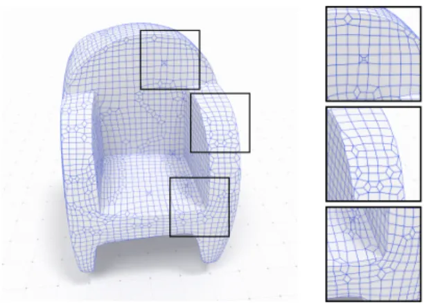
in Figure 2, this surface reconstruction guided by our
piecewise-33
smooth normal vector field effectively aligns quad edges with
34
sharp surface discontinuities.
35
Figure 2: Surface reconstruction obtained from the normal field regularized with our weighted Ambrosio-Tortorelli functional (see Fig.1b for the input voxel grid). The insets show how the quadrangulation perfectly recovers the surface singular-ities.
6. Evaluation 36
We first study the impact of the different components of our 37
method, before comparing it against prior work. For all these 38
results, we use the dataset provided by Delanoy et al. [1] to train 39
the neural networks. This dataset is composed of abstract shapes 40
assembled from cuboids and cylinders, along with line drawings 41
rendered from front, side, top and 3/4 views. Note however that 42
we only train and use the normal map predictor on 3/4 views 43
because the other views are often highly ambiguous. 44
6.1. Ablation study 45
Figure 3 compares the surface reconstructions obtained with 46
different sources of normal guidance, and different strategies of 47
normal fusion. We color surfaces according to their orientations, 48
as shown by the sphere in inset. As a baseline, we first extract the 49
surface best aligned with the gradient of the volumetric predic- 50
tion, similarly to prior work [1]. Because the volumetric predic- 51
tion is noisy and of low resolution, this naive approach produces 52
bumpy surfaces that lack sharp features (second column). Op- 53
timizing the normal field according to the Ambrosio-Tortorelli 54
energy removes some of the bumps, but still produces rounded 55
corners (third column). Aggregating the volumetric and image- 56
based normals into a single normal field produces smoother sur- 57
faces, but yield bevels where the normal maps are misaligned 58
(fourth and fifth column). We improve results by weighting the 59
aggregated normal field according to its confidence, which gives 60
the Ambrosio-Tortorelli energy greater freedom to locate surface 61
discontinuities in ambiguous areas (last column). 62
We further evaluate the importance of our local weighting 63
scheme in Figure 4. We first show surfaces obtained using a 64
constant α in the Ambrosio-Tortorelli energy. A low α produces 65
sharp creases and smooth surfaces but the final shape deviates 66
from the input, as seen on the cylindrical lens of the camera that 67
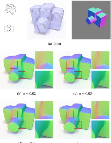
becomes conic (Figure 4b). On the other hand, a high α yields 68
Input voxel surface {ng} {ng}+ AT {¯n} {¯n}+ AT n∗=
{¯n}+ weighted AT
Figure 3: Ablation study showing the surface obtained using various normal fields as guidance. The volumetric gradient ngproduces bumpy surfaces that lack sharp
features (second column), even after being optimized according to the Ambrosio-Tortorelli energy (third column). Our aggregated normal field ¯n yields multiple surface discontinuities where the normal maps are misaligned, such as on the arms and the seat of the armchair (fourth and fifth column). We obtain the best results by reducing the influence of the aggregated normals in areas of low confidence (last column, n∗).
a surface that remain close to the input, but misses some sharp
1
surface transitions (Figure 4d). By defining α as a function of
2
the confidence of the normal field, our formulation produces a
3
surface that is close to the input shape and locates well sharp
4
transitions even in areas where the normal maps are misaligned
5
(Figure 4e).
6
6.2. Performances
7
We implemented the deep networks in Caffe [26] and the
nor-8
mal field and surface optimizations in DGtal1. Both the
predic-9
tion and optimization parts of our method take approximately the
10
same time. The volumetric prediction takes between 150 and 350
11
milliseconds, depending on the number of input sketches [1]. The
12
normal prediction takes around 15 milliseconds per sketch. In
13
contrast, normal field optimization takes around 700 milliseconds
14
and surface optimization takes around 30 milliseconds. Note that
15
we measured our timings using GPU acceleration for the deep
16
networks, while the normal field and surface optimizations were
17
performed on the CPU.
18
Our approach is an order of magnitude faster than prior
image-19
based approaches [3, 2], which need around ten seconds to
per-20
form non-rigid registration and fusion of multiple depth maps.
21
However, our fast normal aggregation strategy is best suited to
22
objects dominated by smooth surface patches delineated by few
23
sharp discontinuities, while it is likely to average out information
24
in the presence of misaligned repetitive details.
25
6.3. Comparisons
26
Figure 5 compares our surfaces with the ones obtained by
De-27
lanoy et al. [1], who apply a marching cube algorithm on the
28
volumetric prediction. Our method produces much smoother
sur-29
faces while capturing sharper discontinuities. While our method
30
benefits from the guidance of the predicted normal maps, it
re-31
mains robust to inconsistencies between these maps and the voxel
32
1https://dgtal.org/
(a) Input
(b) α= 0.02 (c) α= 0.05
(d) α= 0.1 (e) ours
Figure 4: Ambrosio-Tortorelli with a fixed α deviates from the input shape (b) or misses sharp discontinuities (d). Our spatially-varying α allows the recovery of sharp features in areas where the aggregated normal field has a low confidence (e).
grid, as shown on the armchair (top right) where one of the nor- 33
mal maps suggests a non-flat back due to a missing line in the 34
input drawing. 35
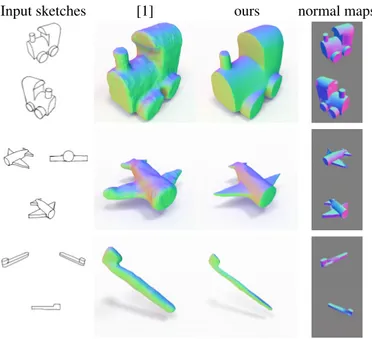
We also provide a comparison to feature-preserving denoising 36
Input sketches [1] [1]+ [27] [1]+ [28] Ours Normal maps
Figure 5: Comparison to Delanoy et al. [1] on a variety of objects. Applying marching cube on the volumetric prediction results in noisy surfaces that lack sharp discontinuities (second column). Denoising these surfaces with L0 minimization [27] introduces spurious discontinuities as curved patches are approximated by planes (third column). Guided denoising [28] produces piecewise-smooth surfaces closer to ours (fourth column) but maintains low-frequency noise and tends to misplace discontinuities, like on the arm of the armchair (second row) or on the wings and front of the airplane (fourth row). Our formulation based on the Ambrosio-Tortorelli energy can be seen as a form of guided filtering that benefits from extra guidance from the predicted normal maps (fifth column). We included close-ups on the input drawings and output surfaces to show that our method better captures the intended shape.
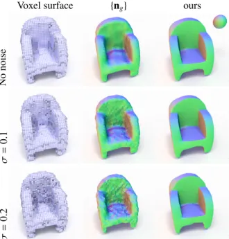
Voxel surface {ng} ours No noise σ = 0 .1 σ = 0 .2
Figure 6: Robustness to noisy volumetric prediction. Adding gaussian noise to the input volumetric prediction has little impact on the final result.
Without normal guidance, these methods either maintain
low-1
frequency noise, remove important features, or introduce
spuri-2
ous discontinuities.
3
6.4. Robustness
4
Figure 6 evaluates the robustness of our method to noisy
volu-5
metric predictions, showing that our combination of normal map
6
guidance and piecewise-smooth regularization yields stable
re-7
sults even in the presence of significant noise. We also designed
8
our method to be robust to normal map misalignment, common
9
in a sketching context. Figure 7 demonstrates that our method is
10
stable in the presence of global and local misalignment. We
sim-11
ulate a global misalignment by shifting one of the normal maps
12
by 5 pixels, and a local misalignment by replacing each normal
13
by another normal, sampled in a local neighborhood.
14
6.5. Limitations
15
Figure 8 illustrates typical limitations of our approach. Since
16
our method relies on normal maps to guide the surface
recon-17
struction, it sometimes misses surface discontinuities between
18
co-planar surfaces, as shown on the top of the locomotive. An
19
additional drawing would be needed in this example to show the
20
discontinuity from bellow. A side effect of the surface
optimiza-21
tion energy is to induce a slight loss of volume, which is
espe-22
cially visible on thin structures like the wings of the airplane and
23
the toothbrush. Possible solutions to this issue includes iterating
24
between regularizing the surface and restoring volume by
mov-25
ing each vertex in its normal direction. Another limitation of our
26
approach is that normal maps only help recovering fine details on
27 {¯n} {¯n}+ AT ours No noise Global shift Local shift
Figure 7: Robustness to misaligned normal maps. Here we simulate global mis-alignment by shifting an entire normal map by the same amount (second row) or by shifting each normal by a random amount (third row). While these perturba-tions degrades the result of the baseline methods, our method remains stable.
visible surfaces, while hidden parts are solely reconstructed from 28
the volumetric prediction, as shown on the back of the camera in 29
Figure 9. Finally, because we favor piecewise-smooth surfaces, 30
our approach is better suited to man-made objects than to organic 31
shapes made of intricate details. 32
7. Conclusion 33
Recent work on sketch-based modeling using deep learning 34
relied either on volumetric or image-based representations of 3D 35
shapes. In this paper we showed how these two representations 36
can be combined, using the volumetric representation to capture 37
hidden parts and the image-based representation to capture sharp 38
details. Furthermore, we showed how the volumetric represen- 39
tation can serve as a support for normal map fusion by solving 40
for a piecewise-smooth normal field over the voxel surface. This 41
method is especially well suited to man-made objects dominated 42
by a few sharp discontinuities. 43
Acknowledgments 44
This work was supported in part by the ERC starting grant D3 45
(ERC-2016-STG 714221), CoMeDiC research grant (ANR-15- 46
CE40-0006), research and software donations from Adobe, and 47
by hardware donations from NVIDIA. The authors are grateful to 48
Inria Sophia Antipolis - M´editerran´ee ”Nef” computation cluster 49
Input sketches [1] ours normal maps
Figure 8: Limitations of our method. Our method cannot recover surface dis-continuities that are not captured by the normal maps, such as the top of the locomotive. The surface optimization tends to shrink the object, as seen on thin structures like the wings of the airplane and the toothbrush.
Figure 9: Since normal maps only capture visible surfaces, the back and bottom of this camera is solely defined by the volumetric prediction. Nevertheless, the method reconstructs a smooth surface in such cases as it still benefits from the piecewise-smoothness of the Ambrosio-Tortorelli energy.
References
1
[1] Delanoy, J, Aubry, M, Isola, P, Efros, AA, Bousseau,
2
A. 3d sketching using multi-view deep volumetric
predic-3
tion. Proceedings of the ACM on Computer Graphics and
4
Interactive Techniques 2018;1(1):21.
5
[2] Lun, Z, Gadelha, M, Kalogerakis, E, Maji, S, Wang,
6
R. 3d shape reconstruction from sketches via multi-view
7
convolutional networks. In: IEEE International Conference
8
on 3D Vision (3DV). 2017, p. 67–77.
9
[3] Li, C, Pan, H, Liu, Y, Tong, X, Sheffer, A, Wang,
10
W. Robust flow-guided neural prediction for sketch-based
11
freeform surface modeling. In: ACM Transaction on 12
Graphics (Proc. SIGGRAPH Asia). ACM; 2018, p. 238. 13
[4] Su, W, Du, D, Yang, X, Zhou, S, Fu, H. Interactive 14
sketch-based normal map generation with deep neural net- 15
works. Proceedings of the ACM on Computer Graphics and 16
Interactive Techniques 2018;1(1). 17
[5] Coeurjolly, D, Foare, M, Gueth, P, Lachaud, JO. Piece- 18
wise smooth reconstruction of normal vector field on digital 19
data. In: Computer Graphics Forum; vol. 35. Wiley Online 20
Library; 2016, p. 157–167. 21
[6] Coeurjolly, D, Gueth, P, Lachaud, JO. Digital surface 22
regularization by normal vector field alignment. In: Inter- 23
national Conference on Discrete Geometry for Computer 24
Imagery. Springer; 2017, p. 197–209. 25
[7] Barrow, H, Tenenbaum, J. Interpreting line drawings as 26
three-dimensional surfaces. Artificial Intelligence 1981;17. 27
[8] Xu, B, Chang, W, Sheffer, A, Bousseau, A, McCrae, J, 28
Singh, K. True2form: 3d curve networks from 2d sketches 29
via selective regularization. ACM Transactions on Graphics 30
(Proc SIGGRAPH) 2014;33(4). 31
[9] Malik, J, Maydan, D. Recovering three-dimensional shape 32
from a single image of curved objects. IEEE Pattern Analy- 33
sis and Machine Intelligence (PAMI) 1989;11(6):555–566. 34
[10] Schmidt, R, Khan, A, Singh, K, Kurtenbach, G. Analytic 35
drawing of 3d scaffolds. In: ACM Transactions on Graphics 36
(Proc. SIGGRAPH Asia); vol. 28. ACM; 2009, p. 149. 37
[11] Lipson, H, Shpitalni, M. Optimization-based reconstruc- 38
tion of a 3d object from a single freehand line drawing. 39
Computer-Aided Design 1996;28(8):651–663. 40
[12] Nishida, G, Garcia-Dorado, I, G. Aliaga, D, Benes, B, 41
Bousseau, A. Interactive sketching of urban procedu- 42
ral models. ACM Transactions on Graphics (Proc SIG- 43
GRAPH) 2016;. 44
[13] Huang, H, Kalogerakis, E, Yumer, E, Mech, R. Shape 45
synthesis from sketches via procedural models and convo- 46
lutional networks. IEEE Transactions on Visualization and 47
Computer Graphics (TVCG) 2016;22(10):1. 48
[14] Han, X, Gao, C, Yu, Y. Deepsketch2face: A deep learn- 49
ing based sketching system for 3d face and caricature mod- 50
eling. ACM Transactions on Graphics (Proc SIGGRAPH) 51
2017;36(4). 52
[15] Choy, CB, Xu, D, Gwak, J, Chen, K, Savarese, S. 53
3d-r2n2: A unified approach for single and multi-view 3d 54
object reconstruction. In: IEEE European Conference on 55
Computer Vision (ECCV). 2016, p. 628–644. 56
[16] Ji, M, Gall, J, Zheng, H, Liu, Y, Fang, L. Surfacenet:
1
An end-to-end 3d neural network for multiview
stereop-2
sis. In: IEEE International Conference on Computer Vision
3
(ICCV). 2017,.
4
[17] Tatarchenko, M, Dosovitskiy, A, Brox, T. Multi-view 3d
5
models from single images with a convolutional network.
6
In: European Conference on Computer Vision (ECCV).
7
2016,.
8
[18] Tatarchenko, M, Dosovitskiy, A, Brox, T. Octree
gen-9
erating networks: Efficient convolutional architectures for
10
high-resolution 3d outputs. In: IEEE International
Confer-11
ence on Computer Vision (ICCV). 2017, p. 2088–2096.
12
[19] H¨ane, C, Tulsiani, S, Malik, J. Hierarchical surface
pre-13
diction for 3d object reconstruction. In: IEEE International
14
Conference on 3D Vision (3DV). 2017, p. 412–420.
15
[20] Fan, H, Su, H, Guibas, L. A point set generation network
16
for 3d object reconstruction from a single image. IEEE
17
Computer Vision and Pattern Recognition (CVPR) 2017;.
18
[21] Wang, N, Zhang, Y, Li, Z, Fu, Y, Liu, W, Jiang, YG.
19
Pixel2mesh: Generating 3d mesh models from single rgb
20
images. In: European Conference on Computer Vision
21
(ECCV). 2018,.
22
[22] Bronstein, MM, Bruna, J, LeCun, Y, Szlam, A,
Van-23
dergheynst, P. Geometric deep learning: Going
be-24
yond euclidean data. IEEE Signal Processing Magazine
25
2017;34(4):18–42.
26
[23] Groueix, T, Fisher, M, Kim, VG, Russell, BC, Aubry, M.
27
Atlasnet: A papier-mˆach´e approach to learning 3d surface
28
generation. In: IEEE Conference on Computer Vision and
29
Pattern Recognition (CVPR). 2018, p. 216–224.
30
[24] Isola, P, Zhu, JY, Zhou, T, Efros, AA. Image-to-image
31
translation with conditional adversarial networks. IEEE
32
Conference on Computer Vision and Pattern Recognition
33
(CVPR) 2017;.
34
[25] Ronneberger, O, Fischer, P, Brox, T. U-net: Convolutional
35
networks for biomedical image segmentation. In:
Medi-36
cal Image Computing and Computer-Assisted Intervention
37
- MICCAI. 2015, p. 234–241.
38
[26] Jia, Y, Shelhamer, E, Donahue, J, Karayev, S, Long, J,
39
Girshick, R, et al. Caffe: Convolutional architecture for fast
40
feature embedding. arXiv preprint arXiv:14085093 2014;.
41
[27] He, L, Schaefer, S. Mesh denoising via l 0 minimization.
42
ACM Transactions on Graphics (TOG) 2013;32(4):64.
43
[28] Zhang, W, Deng, B, Zhang, J, Bouaziz, S, Liu, L.
44
Guided mesh normal filtering. In: Computer Graphics
Fo-45
rum; vol. 34. Wiley Online Library; 2015, p. 23–34.
![Figure 5: Comparison to Delanoy et al. [1] on a variety of objects. Applying marching cube on the volumetric prediction results in noisy surfaces that lack sharp discontinuities (second column)](https://thumb-eu.123doks.com/thumbv2/123doknet/13630108.426391/7.918.114.807.104.1015/comparison-delanoy-applying-marching-volumetric-prediction-surfaces-discontinuities.webp)