HAL Id: hal-01952458
https://hal.inria.fr/hal-01952458
Submitted on 13 Dec 2018
HAL is a multi-disciplinary open access
archive for the deposit and dissemination of sci-entific research documents, whether they are pub-lished or not. The documents may come from teaching and research institutions in France or
L’archive ouverte pluridisciplinaire HAL, est destinée au dépôt et à la diffusion de documents scientifiques de niveau recherche, publiés ou non, émanant des établissements d’enseignement et de recherche français ou étrangers, des laboratoires
Deep Learning with Mixed Supervision for Brain Tumor
Segmentation
Pawel Mlynarski, Hervé Delingette, Antonio Criminisi, Nicholas Ayache
To cite this version:
Pawel Mlynarski, Hervé Delingette, Antonio Criminisi, Nicholas Ayache. Deep Learning with Mixed Supervision for Brain Tumor Segmentation. Journal of Medical Imaging, SPIE Digital Library, 2019, �10.1117/1.JMI.6.3.034002�. �hal-01952458�
Deep Learning with Mixed Supervision for Brain Tumor
Segmentation
Pawel Mlynarskia, Herv´e Delingettea, Antonio Criminisib, Nicholas Ayachea
aUniversit´e Cˆote d’Azur, Inria Sophia Antipolis, France. bMicrosoft Research Cambridge, United Kingdom.
Abstract
Most of the current state-of-the-art methods for tumor segmentation are based on machine learning models trained on manually segmented images. This type of training data is particularly costly, as manual delineation of tumors is not only time-consuming but also requires medical expertise. On the other hand, images with a provided global label (indicating presence or absence of a tumor) are less informative but can be obtained at a substan-tially lower cost. In this paper, we propose to use both types of training data (fully-annotated and weakly-annotated) to train a deep learning model for segmentation. The idea of our approach is to extend segmentation net-works with an additional branch performing image-level classification. The model is jointly trained for segmentation and classification tasks in order to exploit information contained in weakly-annotated images while prevent-ing the network to learn features which are irrelevant for the segmentation task. We evaluate our method on the challenging task of brain tumor seg-mentation in Magnetic Resonance images from BRATS 2018 challenge. We show that the proposed approach provides a significant improvement of seg-mentation performance compared to the standard supervised learning. The observed improvement is proportional to the ratio between weakly-annotated and fully-annotated images available for training.
Keywords: Semi-supervised learning, Convolutional Neural Networks, segmentation, tumor, MRI
1. Introduction
Cancer is today the third cause of mortality worldwide. In this paper, we focus on segmentation of gliomas, which are the most frequent primary brain
cancers [1]. Gliomas are particularly malignant tumors and can be broadly classified according to their grade into low grade gliomas (grades I and II defined by World Health Organization) and high grades gliomas (grades III-IV). Glioblastoma multiforme is the most malignant form of glioma and is associated with a very poor prognosis: the average survival time under therapy is between 12 and 14 months.
Medical images play a key role in diagnosis, therapy planning and mon-itoring of cancers. Treatment protocols often include evaluation of tumor volumes and locations. In particular, for radiotherapy planning, clinicians have to manually delineate target volumes, which is a difficult and time-consuming task. Magnetic Resonance (MR) images [2] are particularly suit-able for brain cancer imaging. Different MR sequences (T2, T2-FLAIR, T1, T1+gadolinium) highlight different tumor subcomponents such as edema, necrosis or contrast-enhancing core.
In recent years, machine learning methods have achieved impressive per-formance in a large variety of image recognition tasks. Most of the recent state-of-the-art segmentation methods are based on Convolutional Neural Networks (CNN) [3, 4]. CNNs have the considerable advantage of automati-cally learning relevant image features. This ability is particularly important for the tumor segmentation task. CNN-based methods [5, 6, 7, 8] have ob-tained the best performances on the four last editions of Multimodal Brain Tumor Segmentation Challenge (BRATS) [9, 10].
Most of the segmentation methods based on machine learning rely uniquely on manually segmented images. The cost of this annotation is particu-larly high in medical imaging where manual segmentation is not only time-consuming but also requires high medical competences. Image intensity of cancerous tissues in MRI or CT scans is often similar to the one of surround-ing healthy or pathological tissues, maksurround-ing the exact tumor delineation dif-ficult and subjective. In the case of brain tumors, according to [9], the inter-rater overlap of expert segmentations is between 0.74 and 0.85 in terms of Dice coefficient. For these reasons, high-quality manual tumor segmentations are generally available in very limited numbers. Segmentation approaches able to exploit images with weaker forms of annotations are therefore of particular interest.
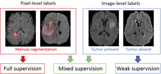
In this paper, we assume that the training dataset contains two types of images: fully-annotated (with provided ground truth segmentation) and weakly-annotated, with an image-level label indicating presence or absence of a tumor tissue within the image (Fig. 1). We refer to this setting as ’mixed
Figure 1: Different levels of supervision for training of segmentation models. Stan-dard models are trained on fully-annotated images only, with pixel-level labels. Weakly-supervised approaches aim to train models using only weakly-annotated images, e.g. with image-level labels. Our model is trained with a mixed supervision, exploiting both types of training images.
supervision’. The latter type of annotations can be obtained at a substan-tially lower cost as it is less time-consuming, potensubstan-tially requires less medical expertise and can be obtained without the use of a dedicated software.
We introduce a novel CNN-based segmentation model which can be trained using weakly-annotated images in addition to fully-annotated images. We propose to extend segmentation networks, such as U-Net [11], with an ad-ditional branch, performing image-level classification. The model is trained jointly for both tasks, on fully-annotated and weakly-annotated images. The goal is to exploit the representation learning ability of CNNs to learn from weakly-annotated images while supervising the training using fully-annotated images in order to learn features relevant for the segmentation task. Our approach differs from the standard semi-supervised learning as we consider weakly-annotated data instead of totally unlabelled data. To the best of our knowledge, we are the first to combine pixel-level and image-level labels for training of models for tumor segmentation.
We perform a series of cross-validated tests on the challenging task of segmentation of gliomas in MR images from BRATS 2018 challenge. We evaluate our model both for binary and multiclass segmentation using a vari-able number of ground truth segmentations availvari-able for training. Since all
3D images from the BRATS 2018 contain brain tumors, we focus on the 2D problem of tumor segmentation in axial slices of a MRI and we assume slice-level labels for weakly-annotated images. Using approximately 220 MRI with slice-level labels and a varying number of fully-annotated MRI, we show that our approach significantly improves the segmentation accuracy when the number of fully-annotated cases is limited.
2. Related work
In the literature, there are several works related to weakly-supervised and semi-supervised learning for object segmentation or detection. Most of the related works were applied to natural images.
The first group of weakly-supervised methods aims to localize objects using only weakly-annotated images for training. When only image-level labels are available, one approach is to design a neural network which outputs two feature maps per class (interpreted as ’heat maps’ of the class) which are then pooled to obtain an image-level classification score penalized during the training [12, 13, 14, 15, 16]. At test time, these ’heat maps’ are used for detection (determining a bounding box of the object) or segmentation. To guide the training process, some works use self-generated spatial priors [13, 14, 15] or inconsistency measures [16] in the loss function. To obtain an image-level score, in [12, 15], global maximum pooling is used. Application of the maximum function on large feature maps may cause optimization problems as training of neural networks is based on computation of gradients [17]. LogSumExp approximation of the maximum [18] is therefore used in the works [13, 14] in order to partially limit this problem. Average pooling on small feature maps was used by Wang et al [16] for the problem of detection of lung nodules.
Another type of weakly-supervised methods aims to detect objects in natural images based on classification of image subregions [19, 20] using pre-trained classification networks such as VGG-Net [21] or AlexNet [22]. In fact, one particularity of natural images is their recursive aspect: one image can correspond to a subpart of another image (e.g. two images of the same object taken from different distances). A classification network trained on a large dataset may therefore be used on a subregion of a new image in order to determine if it contains an object of interest.
Pre-trained classification networks were also used to detect objects by determining image subregions whose modification influences the global
clas-sification score of a class. In [23], Simonyan et al. propose to compute the gradient of the classification score with respect to the intensities of pixels and to threshold it in order to localize the object of interest. However, these partial derivatives represent a very weak information for tumor segmenta-tion, which requires a complex analysis of the spatial context. The method proposed in [24] is based on replacing image subregions by the mean value in order to measure the drop of the classification score.
Overall, the reported segmentation performances of weakly-supervised methods are considerably lower than the ones obtained by semi-supervised and supervised approaches. In absence of pixel-level labels, a model may learn irrelevant features, due for example to co-occurrences of objects or image acquisition differences in the case of multicenter medical data. Despite the cost of manual segmentation, at least few fully-annotated images can still be obtained in many cases.
In standard semi-supervised learning [25] for classification, the training data is composed both of labelled samples and unlabelled samples. Unla-belled samples can be used to encourage the model to satisfy some proper-ties on relations between labels and the feature space. Common properproper-ties include smoothness (points close in the feature space should be close in the target space), clustering (labels form clusters in the feature space) and low density separation (decision boundaries should be in low density regions of the feature space). Semi-supervised learning based on these properties can be performed by graph-based methods such as the recent work of Kamnit-sas et al. [26]. The main idea of such methods is to propagate labels in a fully-connected graph whose nodes are samples (labelled and unlabelled) and whose edges are weighted by similarities between samples. The use of graph-based semi-supervised methods is difficult for segmentation, in partic-ular because it implies computation of similarity metrics between samples, whereas each single image is generally composed of millions of samples (pixels or voxels).
Relatively few works were proposed for semi-supervised learning for image segmentation. Some semi-supervised approaches are based on self-training, i.e. training of a machine learning model on self-generated labels. Itera-tive algorithms similar to EM [27] were proposed for natural images [28] and medical images [29]. Recently, Hung et al [30] proposed a method based on Generative Adversarial Networks [31] where the generator network performs image segmentation and the discriminator network tries to determine if a seg-mentation corresponds to the ground truth or the segseg-mentation produced by
the generator. The discriminator network is used to produce confidence maps for self-training. The approaches based on self-training have the drawback of learning on uncertain labels (produced by the model itself) and training of such models is difficult.
Other approaches assume mixed levels of supervision similarly to our approach. Hong et al [32, 33] proposed decoupled classification and segmen-tation, an approach for segmentation of objects in natural images based on a two-step training with a varying level of supervision. This architecture is composed of two separate networks trained sequentially, one performing image-level classification and used as encoder, and the another one taking as input small feature maps extracted from the encoder and performing seg-mentation. An important drawback of such design, in the case of tumor segmentation, is that the segmentation network does not take as input the original image and can therefore miss important details of the image (e.g. small tumors).
Our approach is related to multi-task learning [34]. In our case, the goal of training for two tasks (segmentation and classification) is to exploit all the available labels and to guide the training process to learn relevant features. The approach closest to ours is the one of Shah et al. [35]. In this work, the authors consider three types of annotations: segmentations, bounding boxes and seed points at the borders of objects. A neural network is trained using these three types of training data. In our work, we exploit the use of a significantly weaker form of annotations, image-level labels.
3. Joint classification and segmentation with Convolutional Neural Networks
3.1. Deep learning model for binary segmentation
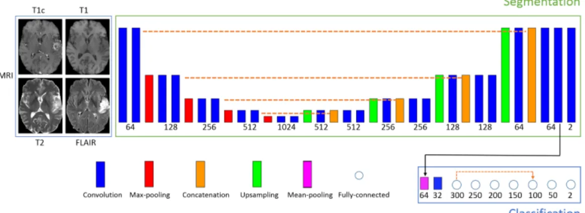
We designed a novel deep learning model, which aims to take advantage of all available voxelwise and image-level annotations. We propose to extend a segmentation CNN with an additional subnetwork performing image-level classification and to train the model for the two tasks jointly. Most of the layers are shared between the classification and segmentation subnetworks in order to transfer the information between the two subnetworks. In this paper we present the 2D version of our model, which can be used on different types of medical images such as slices of a CT scan or a multisequence MRI. The proposed network takes as input an image of dimensions 300x300 and extends U-net [11] which is currently one of the most used architectures
for segmentation tasks in medical imaging. This segmentation architecture is composed of an encoder part and a decoder part which are connected by concatenations between layers at the same scale, in order to combine low-level and local features with high-low-level and global features. This design is well suited for the tumor segmentation task since the classification of a voxel as tumor requires to compare its value with its close neighborhood but also taking into account a large spatial context. The last convolutional layer of U-net produces pixelwise classification scores, which are normalized by softmax function during the training phase. We apply batch normalization [36] in all convolutional layers except the final layer.
We propose to add an additional branch to the network, performing image-level classification (Fig. 2), in order to exploit the information con-tained in weakly-annotated images during the training. This classification branch takes as input the second to last convolutional layer of U-net (rep-resenting a rich information extracted from a local and a long-range spatial context) and is composed of one mean-pooling, one convolutional layer and 7 fully-connected layers.
The goals of taking a layer from the final part of U-Net as input of the classification branch are both to guide the image-level classification task and to force the major part of the segmentation network to take into account
Figure 2: Architecture of our model for binary segmentation. The numbers of outputs are specified below boxes representing layers. The height of rectangles represents the scale (increasing with pooling operations). The dashed lines represent concatenation operations. The proposed architecture is an extended version of U-net, with a subnetwork performing image-level classification. Training of the model corresponds to a joint minimization of two loss functions related respectively to segmentation and image-level classifcation tasks.
weakly-annotated images. This also helps the optimization process by taking advantage of the connectivity of layers in U-Net, helping the flow of gradients of the loss function during the training (in particular, note the connection between the first part and the last part of U-Net).
The second to last layer of the segmentation network outputs 64 feature maps of size 101x101 from which the classification branch has to output two global (image-level) classification scores (tumor absent/tumor present). We first reduce the size of these feature maps by applying a mean-pooling with kernels of size 8x8 and the stride of 8x8. We use the mean pooling rather than max-pooling in order to avoid information loss and optimization problems. One convolutional layer, with ReLU activation and kernels of size 3x3, is then added to reduce the number of feature maps from 64 to 32. The resulting 32 feature maps of size 11x11 are the input of the first fully-connected layer of the classification branch.
According to our experiments, a relatively deep architecture of the clas-sification branch with a limited number of parameters and a skip-connection between layers yields the best performance. This observation is in agreement with current common designs of neural networks. Deep networks have the capacity to learn more complex features, due to applied non-linearities. The connectivity between layers at different depths helps the optimization pro-cess (e.g. Res-Net [37]). In our case, we use 7 fully-connected layers with ReLU activations (except the final layer) and we concatenate the outputs of the first and the fifth fully-connected layer. The last fully-connected layer outputs image-level classification scores (tumor tissue absent or present).
The model is trained both on fully-annotated and weakly-annotated im-ages for the two tasks jointly (segmentation and classification). We can distinguish between three types of training images. First, images containing a tumor and with provided ground truth segmentation are the most costly ones. The second type are images that do not contain tumor, which implies that none of their pixels corresponds to a tumor. In this case, the ground truth segmentation is simply the zero matrix. The only problematic case is the third one, when the image is labelled as containing a tumor but without provided segmentation.
To train our model, we propose to form training batches containing the three mentioned types of images: k positive cases (containing a tumor) with provided segmentation, m negative cases and n positive cases without pro-vided segmentation. In our experiments we chose k = 4, m = 2, n = 4.
pixelwise cross-entropy loss on images of types 1 and 2: Lossbs(θ) = −1 P k+m X i=1 X (x,y)
w(x,y)i log(pli,(x,y)(θ)) (1)
where P is the number of pixels; pl
i,(x,y) is the classification score given by the network to the ground truth label for pixel (x,y) of the ithimage of the batch and w(x,y)i is the weight given to this pixel. The weights are used to limit the effect of class imbalance, since tumor pixels represent a small portion of the image. Weights of pixels are set automatically according to the composition of the training batch (number of pixels of each class) so that pixels associated with healthy tissues have a total weight of t0in the loss function and the pixels of the tumor class have a total weight of t1, where t0 and t1 are target weights fixed manually (t0 = 0.7 and t1 = 0.3 in our experiments). It means that if the training batch contains Nt pixels labelled as tumor, then each tumor pixel has a weight of t1/N1 (the pixelwise weight is high when the number of tumor pixels is low). We fix a higher target weight for healthy tissues to avoid oversegmentation, while increasing the relative weight of tumor pixels (t1 = 0.3) compared to the standard non-weighted cross-entropy loss where the relative weight of the tumor class is proportional to the number of tumor pixels, i.e approximately 1-2 %. This type of loss function was used in our previous work [38].
The classification loss is a standard cross-entropy loss on all images of the training batch: Lossc = −k+m+n1 Pk+m+ni=1 log(pli(θ)) where pli is the global classification score given by the network to the ground truth global label for the ithimage of the batch. In particular, fully-annotated images are also used for training of the classification branch in order to transfer the knowledge from the segmentation task to the image-level classification. We do not apply weights on the classification loss as image-level labels are balanced through the sampling of training batches (having a fixed number of non-tumor images).
Since both segmentation and classification losses are normalized, we de-fine the total loss as a convex combination of the classification and segmen-tation losses: Loss = a ∗ Losss + (1 − a) ∗ Lossc. In our experiments we fixed a=0.7, i.e. we give a higher importance to segmentation errors. The determination of this parameter was performed empirically through a series of cross-validated tests.
We train our model with a variant of Stochastic Gradient Descent (SGD) with momentum [39], used also in our previous work [38]. The main dif-ferences with the standard SGD are to divide the gradient by its norm and to compute gradients on several training batches in each iteration, in order to take into account many training examples while bypassing GPU memory constraints.
3.2. Extension to the multiclass problem
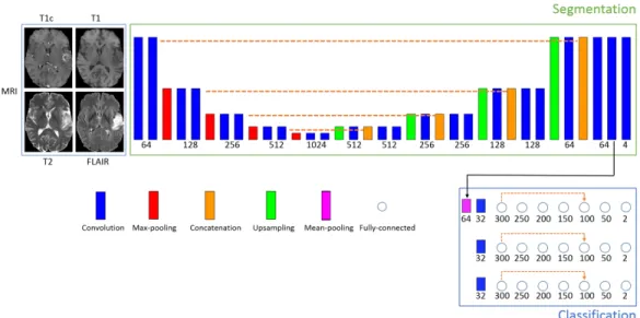
We extend our model to the multiclass case where each pixel has to be labelled with one of K classes, such as the four ones considered in BRATS challenge (non-tumor, contrast-enhancing core, edema, non-enhancing core). We now assume that image-level labels are provided for each class (ab-sent/present in the image).
Extension of the segmentation subnetwork to the multiclass problem is straightforward, by changing the number of final feature maps to match the number of classes. However, image-level labels are not exclusive, i.e. an image may contain several tumor subclasses. For this reason, we propose to consider one image-level classification output per tumor subclass, indicating absence or presence of the given subclass.
According to our experiments, better performances are obtained when each subclass has its dedicated entire classification branch (Fig. 3). A pos-sible reason is that the image-level classification of tumor subclasses is a challenging task requiring a sufficient number of dedicated parameters.
Training batches are sampled similarly to the binary case, however each tumor subclass has to be present at least once in each training batch. In our implementation, we store lists of paths of images containing tumor subclasses in order to sample from these lists during the training of the model.
In the segmentation loss we empirically fix the following target weights for the four classes (non-tumor, non-enhancing tumor core, edema, enhancing-core): t0 = 0.7, t1 = 0.1, t2 = 0.1, t3 = 0.1 (all tumor subclasses have an equal weight in the loss function). The loss associated with each classification branch is the same as in the binary case and the total classification loss is the average across all classification branches. We observe the need to decrease the parameter a (weight of the segmentation loss) compared to the binary case. We fixed a = 0.3 according to performed cross-validated experiments.
Figure 3: Extension of our model to the multiclass problem. The number of final feature maps of the segmentation subnetwork is equal to the number of classes (4 in our case). As image-level labels (class present/absent) are not exclusive, we consider one classification branch per tumor subclass.
4. Experiments 4.1. Data
We evaluate our method on the challenging task of brain tumor segmenta-tion in multisequence MR scans, using the Training dataset of BRATS 2018 challenge. It contains 285 multisequence MRI of patients diagnosed with low-grade gliomas or high-low-grade gliomas. For each patient, manual ground truth segmentation is provided. In each case, four MR sequences are available: T1, T1+gadolinium, T2 and FLAIR (Fluid Attenuated Inversion Recovery). Pre-processing performed by the organizers includes skull-stripping, resampling to 1 mm3 resolution and registration of images to a common brain atlas. The resulting volumes are of size 240x240x155. The images were acquired in 19 different imaging centers. In order to normalize image intensites, each image is divided by the median of non-zero voxels (which is supposed to be less affected by the tumor zone than the mean) and multiplied the image by a fixed constant.
Each voxel is labelled with one of the following classes: non-tumor (class 0), contrast-enhancing core (class 3), non-enhancing core (class 1), edema (class 2). The benchmark of the challenge groups classes in three regions:
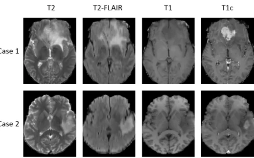
Figure 4: Examples of multisequence MRI from the BRATS 2018 database. While T2 and T2-FLAIR highlight the edema induced by the tumor, T1 is suitable for determining the tumor core. In particular, T1 acquired after injection of a contrast product (T1c) highlights the tumor angiogenesis, indicating presence of highly proliferative cancer cells.
whole tumor (all tumor subclasses), tumor core (classes 1 and 3, correspond-ing to the visible tumor mass) and enhanccorrespond-ing core (class 3).
Given that all 3D images of the database contain tumors (no negative cases to train a 3D classification network), we consider the 2D problem of tumor segmentation in axial slices of the brain.
4.2. Test setting
The goal of our experiments is to compare our approach with the stan-dard supervised learning. In each of the performed tests, our model is trained on fully-annotated and weakly-annotated images and is compared with the standard U-Net trained on fully-annotated images only. The goal is to com-pare our model with a commonly used segmentation model on a publicly available database.
We consider three different training scenarios, with a varying number of patients for which we assume a provided manual tumor segmentation. In each scenario we perform a 5-fold cross-validation. In each fold, 57 patients are used for test and 228 patients are used for training. Among the 228 training images, few cases are assumed to be fully-annotated and the remaining ones
are considered to be weakly-annotated, with slice-level labels. The fully-annotated images are different in each fold. If the 3D volumes are numbered from 0 to 284, then in kthfold, the test images correspond to the interval [(k-1)*57, k*57 -1], the next few images correspond to fully-annotated images and the remaining ones are considered as weakly-annotated (the folds are generated in a circular way). In the following, FA denotes the number of fully-annotated cases and WA denotes the number of weakly-annotated cases (with slice-level labels).
In the first training scenario, 5 patients are assumed to be provided with a manual segmentation and 223 patients have slice-level labels. In the second and the third scenario, the numbers of fully-annotated cases are respectively 15 and 30 and the numbers of weakly-annotated images are therefore re-spectively 213 and 198. The three training scenarios are independent, i.e. folds are re-generated randomly (the list of all images is permuted randomly and the folds are generated). In fact, results are likely to depend not only on the number of fully-annotated images but also on qualitative factors (for example the few fully-annotated images may correspond to atypical cases), and the goal is to test the method in various settings. Overall, our approach is compared to the standard supervised learning on 60 tests (5-fold cross-validation, three independent training scenarios, three binary problems and one multiclass problem).
We evaluate our method both on binary segmentations problems (sepa-rately for each of three tumor regions considered in the challenge) and on the end-to-end multiclass segmentation problem. In each binary case, the model is trained for segmentation and classification of one tumor region (whole tumor, tumor core or enhancing core).
Segmentation performance is expressed in terms of Dice score quantifying the overlap between the ground truth (Y ) and the output of a model ( ˜Y ):
DSC( ˜Y , Y ) = 2| ˜Y ∩ Y |
| ˜Y | + |Y | (2) 4.3. Results
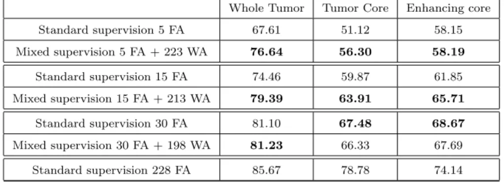
The main observation is that our model with mixed supervision provides a significant improvement over the standard supervised approach (U-Net trained on fully-annotated images) when the number of fully-annotated im-ages is limited. In the two first training scenarios (5 FA and 15 FA), our model outperformed the supervised approach on the three binary segmenta-tion problems (Table 1) and in the multiclass setting (Table 3). The largest
Table 1: Mean Dice scores (5-fold cross-validation, 57 test cases in each fold) in the three binary segmentation problems obtained by the standard supervised approach and by our model trained with mixed supervision.
Whole Tumor Tumor Core Enhancing core Standard supervision 5 FA 70.39 48.14 55.74 Mixed supervision 5 FA + 223 WA 78.34 50.11 60.06 Standard supervision 15 FA 77.91 58.33 62.88 Mixed supervision 15 FA + 213 WA 80.92 63.23 66.61 Standard supervision 30 FA 83.95 66.17 69.15 Mixed supervision 30 FA + 198 WA 83.84 68.30 67.18 Standard supervision 228 FA 86.80 77.09 72.20
Table 2: Results obtained for the three binary problems (whole tumor, tumor core, en-hancing core) on different folds in the case with 15 fully-annotated images and 213 weakly-annotated images.
fold1 fold2 fold3 fold4 fold5 mean Standard supervision, whole tumor 76.23 78.15 78.13 77.67 79.35 77.91 Mixed supervision, whole tumor 82.36 81.03 78.96 79.88 82.35 80.92 Standard supervision, tumor core 61.46 61.17 56.68 56.42 55.94 58.33 Mixed supervision, tumor core 63.15 66.82 63.45 60.83 61.91 63.23 Standard supervision, enhancing core 66.33 61.08 57.86 68.09 61.02 62.88 Mixed supervision, enhancing core 68.72 70.65 60.34 67.55 65.80 66.61
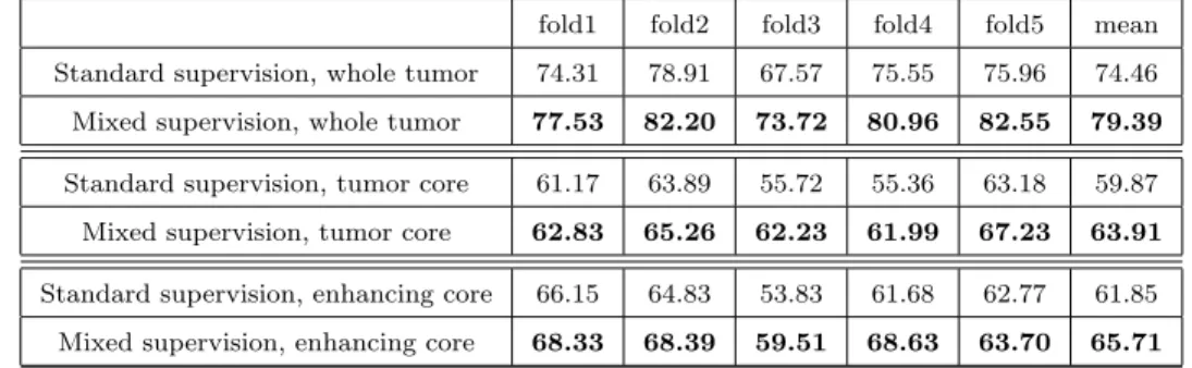
improvements are in the first scenario (5 FA) for the whole tumor region where the improvement is of 8 points of the mean Dice score in the binary setting and of 9 points of Dice in the multiclass setting. Results on different folds of the second scenario (intermediate case, 15 FA) are displayed in Table 2 for the binary problems and in Table 4 for the multiclass problem. Our approach provided an improvement in all folds of the second scenario and for all tumor regions, except one fold for enhancing core in the binary setting. In the third scenario (30 FA + 198 WA), our approach and the standard supervised approach obtained similar performances.
Segmentation performance increases quickly with the first fully-annotated cases, both for the standard supervised learning and the learning with mixed supervision. For instance, mean Dice score obtained by the supervised ap-proach for whole tumor increases from 70.39, in the case with 5 fully-annotated
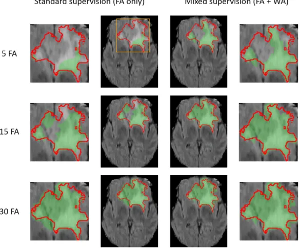
Figure 5: Comparison of our approach with the standard supervised learning for binary segmentation of the ’whole tumor’ region. Each row represents the same test example (first image of Fig. 4) from a different training scenario (5, 15 or 30 fully-annotated scans available for training). FA and WA refer respectively to the number of fully-annotated MRI and weakly-annotated MRI (with slice-level labels). The results are displayed on MRI T2-FLAIR sequence. The performance of both models improves with the number of manual segmentations available for training.
images, to 77.9 in the case with 15 fully-annotated images. Our approach using 5 fully-annotated images and 223 weakly-annotated images obtained a slightly better performance (78.3) than the supervised approach using 15 fully-annotated cases (77.9). This result is represented on Fig. 7.
Note that each fully-annotated case corresponds to a large 3D volume with voxelwise annotations. Each manually segmented axial slice of size 240x240 corresponds to 57 600 labels, which represents indeed a huge amount
Figure 6: Comparison of our approach with the standard supervised learning for binary segmentation of the ’tumor core’ region (test example corresponding to the bottom image of Fig. 4). Each row corresponds to a different training scenario (5, 15 or 30 fully-annotated scans available for training). FA and WA refer to the numbers of fully-fully-annotated and weakly-annotated scans. The results are displayed on MRI T1+gadolinium. The observations are similar to the problem of binary segmentation of the ’whole tumor’ region. In particular, in the first training scenario, the standard supervised approach does not detect the tumor core zone, in contrast to our method.
of information compared to one global label simply indicating presence of absence of a tumor tissue within the slice.
In terms of the annotation cost, manual delineation of tumor tissues in one MRI may take about 45 minutes for an experienced oncologist using a
Figure 7: Illustration of the improvement provided by the mixed supervision for binary segmentation of the ’whole tumor’ region. Mixed supervision using 5 fully-annotated MRI and 223 weakly-annotated MRI obtains a slightly better performance than the standard supervised approach using 15 fully-annotated MRI. The improvement provided by the weakly-annotated images decreases with the number of available ground truth segmenta-tions.
Table 3: Mean Dice scores (5-fold cross-validation, 57 test cases in each fold) obtained by the standard supervised approach and by our model in the multiclass setting.
Whole Tumor Tumor Core Enhancing core Standard supervision 5 FA 67.61 51.12 58.15 Mixed supervision 5 FA + 223 WA 76.64 56.30 58.19 Standard supervision 15 FA 74.46 59.87 61.85 Mixed supervision 15 FA + 213 WA 79.39 63.91 65.71 Standard supervision 30 FA 81.10 67.48 68.67 Mixed supervision 30 FA + 198 WA 81.23 66.33 67.69 Standard supervision 228 FA 85.67 78.78 74.14
Table 4: Results obtained in the multiclass setting on different folds in the case with 15 fully-annotated images and 213 weakly-annotated images.
fold1 fold2 fold3 fold4 fold5 mean Standard supervision, whole tumor 74.31 78.91 67.57 75.55 75.96 74.46 Mixed supervision, whole tumor 77.53 82.20 73.72 80.96 82.55 79.39 Standard supervision, tumor core 61.17 63.89 55.72 55.36 63.18 59.87 Mixed supervision, tumor core 62.83 65.26 62.23 61.99 67.23 63.91 Standard supervision, enhancing core 66.15 64.83 53.83 61.68 62.77 61.85 Mixed supervision, enhancing core 68.33 68.39 59.51 68.63 63.70 65.71
dedicated segmentation tool. Determining the range of axial slices containing tumor tissues may take 1-2 minutes but can be done without a specialized software. More importantly, determining global labels may require less med-ical expertise than performing an exact tumor delineation and can therefore be performed by a larger community.
5. Conclusion and future work
In this paper we proposed a new deep learning approach for tumor seg-mentation which takes advantage of weakly-annotated medical images during the training of neural networks, in addition to a small number of manually segmented images. In our approach, we propose to use neural networks pro-ducing both voxelwise and image-level outputs. The classification and seg-mentation subnetworks share most of their layers and are trained jointly us-ing both fully-annotated and weakly-annotated data. We performed a large number of cross-validated experiments to test our method both in binary and multiclass settings. Our experiments showed that the use of weakly-annotated data improves the segmentation performance significantly when the number of manually segmented images is limited. Our model is end-to-end and straightforward to implement with common deep learning libraries such as Theano [40] or TensorFlow [41]. The code of our method will be made publicly available in order to encourage other researchers to continue the research in the field.
An interesting step of the future work would be to extend our method to an end-to-end 3D segmentation. In our paper we focused on the 2D segmen-tation problem, in particular because all 3D images from the BRATS 2018 database contain tumors whereas we also need non-tumor images to train
the classification part of our model. One advantage of the 3D application would be to take into account a richer spatial context in the case of MRI or CT scans. Furthermore, volume-level labels require less effort than slice-level labels and would therefore be easier to obtain, even if these labels are also less informative.
In our tests, we used approximately 220 weakly-annotated MRI, which is relatively a limited number. An important future step would be to test our method on a database containing a considerably larger number of weakly-annotated images (thousands, millions).
Acknowledgements
Pawel Mlynarski is funded by the Microsoft Research-INRIA Joint Center, France. This work was supported by the Inria Sophia Antipolis - M´editerran´ee, ”NEF” computation cluster.
References
[1] M. L. Goodenberger, R. B. Jenkins, Genetics of adult glioma, Cancer genetics 205 (2012) 613–621.
[2] S. Bauer, R. Wiest, L.-P. Nolte, M. Reyes, A survey of mri-based medical image analysis for brain tumor studies, Physics in medicine and biology 58 (2013) R97.
[3] Y. LeCun, Y. Bengio, et al., Convolutional networks for images, speech, and time series, The handbook of brain theory and neural networks 3361 (1995) 1995.
[4] J. Long, E. Shelhamer, T. Darrell, Fully convolutional networks for semantic segmentation, in: Proceedings of the IEEE Conference on Computer Vision and Pattern Recognition, 2015, pp. 3431–3440. [5] S. Pereira, A. Pinto, V. Alves, C. A. Silva, Deep convolutional neural
networks for the segmentation of gliomas in multi-sequence mri, in: In-ternational Workshop on Brainlesion: Glioma, Multiple Sclerosis, Stroke and Traumatic Brain Injuries, Springer, 2015, pp. 131–143.
[6] K. Kamnitsas, C. Ledig, V. F. Newcombe, J. P. Simpson, A. D. Kane, D. K. Menon, D. Rueckert, B. Glocker, Efficient multi-scale 3d cnn with fully connected crf for accurate brain lesion segmentation, arXiv preprint arXiv:1603.05959 (2016).
[7] K. Kamnitsas, W. Bai, E. Ferrante, S. McDonagh, M. Sinclair, N. Pawlowski, M. Rajchl, M. Lee, B. Kainz, D. Rueckert, et al., En-sembles of multiple models and architectures for robust brain tumour segmentation, arXiv preprint arXiv:1711.01468 (2017).
[8] G. Wang, W. Li, S. Ourselin, T. Vercauteren, Automatic brain tumor segmentation using cascaded anisotropic convolutional neural networks, arXiv preprint arXiv:1709.00382 (2017).
[9] B. H. Menze, A. Jakab, S. Bauer, J. Kalpathy-Cramer, K. Farahani, J. Kirby, Y. Burren, N. Porz, J. Slotboom, R. Wiest, et al., The multi-modal brain tumor image segmentation benchmark (brats), IEEE trans-actions on medical imaging 34 (2015) 1993–2024.
[10] S. Bakas, H. Akbari, A. Sotiras, M. Bilello, M. Rozycki, J. S. Kirby, J. B. Freymann, K. Farahani, C. Davatzikos, Advancing the cancer genome atlas glioma mri collections with expert segmentation labels and radiomic features, Scientific data 4 (2017) 170117.
[11] O. Ronneberger, P. Fischer, T. Brox, U-net: Convolutional networks for biomedical image segmentation, in: International Conference on Medical Image Computing and Computer-Assisted Intervention, Springer, 2015, pp. 234–241.
[12] D. Pathak, E. Shelhamer, J. Long, T. Darrell, Fully convolutional multi-class multiple instance learning, arXiv preprint arXiv:1412.7144 (2014). [13] P. O. Pinheiro, R. Collobert, From image-level to pixel-level labeling with convolutional networks, in: Proceedings of the IEEE Conference on Computer Vision and Pattern Recognition, 2015, pp. 1713–1721. [14] F. Saleh, M. S. Aliakbarian, M. Salzmann, L. Petersson, S. Gould, J. M.
Alvarez, Built-in foreground/background prior for weakly-supervised semantic segmentation, in: European Conference on Computer Vision, Springer, 2016, pp. 413–432.
[15] A. Bearman, O. Russakovsky, V. Ferrari, L. Fei-Fei, Whats the point: Semantic segmentation with point supervision, in: European Conference on Computer Vision, Springer, 2016, pp. 549–565.
[16] Z. Wang, C. Liu, D. Cheng, L. Wang, X. Yang, K.-T. Cheng, Automated detection of clinically significant prostate cancer in mp-mri images based on an end-to-end deep neural network, IEEE transactions on medical imaging 37 (2018) 1127–1139.
[17] S. E. Dreyfus, Artificial neural networks, back propagation, and the kelley-bryson gradient procedure, Journal of Guidance, Control, and Dynamics 13 (1990) 926–928.
[18] S. Boyd, L. Vandenberghe, Convex optimization, Cambridge university press, 2004.
[19] R. Girshick, J. Donahue, T. Darrell, J. Malik, Rich feature hierarchies for accurate object detection and semantic segmentation, in: Proceed-ings of the IEEE conference on computer vision and pattern recognition, 2014, pp. 580–587.
[20] M. Oquab, L. Bottou, I. Laptev, J. Sivic, Is object localization for free?-weakly-supervised learning with convolutional neural networks, in: Proceedings of the IEEE Conference on Computer Vision and Pattern Recognition, 2015, pp. 685–694.
[21] K. Simonyan, A. Zisserman, Very deep convolutional networks for large-scale image recognition, arXiv preprint arXiv:1409.1556 (2014).
[22] A. Krizhevsky, I. Sutskever, G. E. Hinton, Imagenet classification with deep convolutional neural networks, in: Advances in neural information processing systems, 2012, pp. 1097–1105.
[23] K. Simonyan, A. Vedaldi, A. Zisserman, Deep inside convolutional net-works: Visualising image classification models and saliency maps, arXiv preprint arXiv:1312.6034 (2013).
[24] A. Bergamo, L. Bazzani, D. Anguelov, L. Torresani, Self-taught object localization with deep networks, arXiv preprint arXiv:1409.3964 (2014).
[25] V. Cheplygina, M. de Bruijne, J. P. Pluim, Not-so-supervised: a sur-vey of semi-supervised, multi-instance, and transfer learning in medical image analysis, arXiv preprint arXiv:1804.06353 (2018).
[26] K. Kamnitsas, D. C. Castro, L. L. Folgoc, I. Walker, R. Tanno, D. Rueckert, B. Glocker, A. Criminisi, A. Nori, Semi-supervised learn-ing via compact latent space clusterlearn-ing, arXiv preprint arXiv:1806.02679 (2018).
[27] Y. Zhang, M. Brady, S. Smith, Segmentation of brain mr images through a hidden markov random field model and the expectation-maximization algorithm, IEEE transactions on medical imaging 20 (2001) 45–57. [28] G. Papandreou, L.-C. Chen, K. P. Murphy, A. L. Yuille, Weakly-and
semi-supervised learning of a deep convolutional network for semantic image segmentation, in: Proceedings of the IEEE international confer-ence on computer vision, 2015, pp. 1742–1750.
[29] M. Rajchl, M. C. Lee, O. Oktay, K. Kamnitsas, J. Passerat-Palmbach, W. Bai, B. Kainz, D. Rueckert, Deepcut: Object segmentation from bounding box annotations using convolutional neural networks, arXiv preprint arXiv:1605.07866 (2016).
[30] W.-C. Hung, Y.-H. Tsai, Y.-T. Liou, Y.-Y. Lin, M.-H. Yang, Adversar-ial learning for semi-supervised semantic segmentation, arXiv preprint arXiv:1802.07934 (2018).
[31] I. Goodfellow, J. Pouget-Abadie, M. Mirza, B. Xu, D. Warde-Farley, S. Ozair, A. Courville, Y. Bengio, Generative adversarial nets, in: Advances in neural information processing systems, 2014, pp. 2672– 2680.
[32] S. Hong, H. Noh, B. Han, Decoupled deep neural network for semi-supervised semantic segmentation, in: Advances in neural information processing systems, 2015, pp. 1495–1503.
[33] S. Hong, J. Oh, H. Lee, B. Han, Learning transferrable knowledge for semantic segmentation with deep convolutional neural network, in: Proceedings of the IEEE Conference on Computer Vision and Pattern Recognition, 2016, pp. 3204–3212.
[34] T. Evgeniou, M. Pontil, Regularized multi–task learning, in: Proceed-ings of the tenth ACM SIGKDD international conference on Knowledge discovery and data mining, ACM, 2004, pp. 109–117.
[35] M. P. Shah, S. Merchant, S. P. Awate, Ms-net: Mixed-supervision fully-convolutional networks for full-resolution segmentation, in: Interna-tional Conference on Medical Image Computing and Computer-Assisted Intervention, Springer, 2018, pp. 379–387.
[36] S. Ioffe, C. Szegedy, Batch normalization: Accelerating deep net-work training by reducing internal covariate shift, arXiv preprint arXiv:1502.03167 (2015).
[37] K. He, X. Zhang, S. Ren, J. Sun, Deep residual learning for image recognition, in: Proceedings of the IEEE conference on computer vision and pattern recognition, 2016, pp. 770–778.
[38] P. Mlynarski, H. Delingette, A. Criminisi, N. Ayache, 3d convolutional neural networks for tumor segmentation using long-range 2d context, arXiv preprint arXiv:1807.08599 (2018).
[39] D. E. Rumelhart, G. E. Hinton, R. J. Williams, Learning representations by back-propagating errors, Cognitive modeling 5 (1988) 1.
[40] J. Bergstra, O. Breuleux, F. Bastien, P. Lamblin, R. Pascanu, G. Des-jardins, J. Turian, D. Warde-Farley, Y. Bengio, Theano: A cpu and gpu math compiler in python, in: Proc. 9th Python in Science Conf, 2010, pp. 1–7.
[41] M. Abadi, A. Agarwal, P. Barham, E. Brevdo, Z. Chen, C. Citro, G. S. Corrado, A. Davis, J. Dean, M. Devin, et al., Tensorflow: Large-scale machine learning on heterogeneous distributed systems, arXiv preprint arXiv:1603.04467 (2016).