The impact of ambient air pollution on hospital admissions

The Impact of Ambient Air Pollution on Hospital Admissions

Massimo Filippini, Giuliano Masiero, and Sandro Steinbach

Published in:

European Journal of Health Economics (2019), 20: 919–931

<https://doi.org/10.1007/s10198-019-01049-y>

Abstract

Ambient air pollution is the environmental factor with the most significant impact on human

health. Several epidemiological studies provide evidence for an association between ambient

air pollution and human health. However, the recent economic literature has challenged the

identification strategy used in these studies. This paper contributes to the ongoing discussion by

investigating the association between ambient air pollution and morbidity using hospital admission

data from Switzerland. Our identification strategy rests on the construction of geographically

explicit pollution measures derived from a dispersion model that replicates atmospheric conditions

and accounts for several emission sources. The reduced form estimates account for location

and time fixed effects and show that ambient air pollution has a substantial impact on hospital

admissions. In particular, we show that SO2 and NO2 are positively associated with admission

rates for coronary artery and cerebrovascular diseases while we find no similar correlation for

PM10 and O3. Our robustness checks support these findings and suggest that dispersion models

can help in reducing the measurement error inherent to pollution exposure measures based on

station-level pollution data. Therefore, our results may contribute to a more accurate evaluation

of future environmental policies aiming at a reduction of ambient air pollution exposure.

Keywords: Ambient air pollution, dispersion model, hospital admissions, count panel data

JEL Codes: I10, Q51, Q53

Acknowledgement: We thank the Swiss Federal Office for the Environment (FOEN) for providing the ambient air pollution data and the Swiss Federal Statistical Office (FSO) for making available the hospital-ization data. We are grateful to one anonymous reviewer and the editor for constructive suggestions. The corresponding author of this paper is Sandro Steinbach. Massimo Filippini: Department of Management, Technology and Economics (D-MTEC), Swiss Federal Institute of Technology in Zurich (ETH Zurich), Zurich, Switzerland, and Institute of Economics (IdEP), Università della Svizzera Italiana (USI), Lugano, Switzerland email: mfilippini@ethz.ch. Giuliano Masiero: Institute of Economics (IdEP), Università della Svizzera Italiana (USI), Lugano, Switzerland, and Department of Management, Information and Production Engineering (DIGIP), University of Bergamo, Bergamo, Italy, email: giuliano.masiero@usi.ch. Sandro Steinbach: Department of Management, Technology and Economics (D-MTEC), Swiss Federal Institute of Technology in Zurich (ETH Zurich), Switzerland, email: ssteinbach@ethz.ch.

1. Introduction

Even though air quality has improved substantially in the last decades, ambient air pollution is still the environmental factor with the greatest health impact in developed countries. The World Health Organization (WHO) has estimated that exposure to ambient air pollution is responsible for health care expenses of more than US$ 1.27 trillion in Europe alone (WHO Regional Office for Europe and OECD, 2015). The significant decrease in pollution exposure in industrialized countries is largely due to stricter environmental regulations and technological progress. However, a substantial proportion of the European population is still exposed to levels of air pollution that are above national and international air quality standards (European Environmental Agency, 2015). Among those air pollutants, particulate matter (PM), nitrogen dioxide (NO2), sulfur dioxide (SO2), and ground-level ozone (O3) are considered to have the largest health impacts. These pollutants are associated with higher mortality and morbidity rates (WHO, 2005). Although the literature on the relationship between ambient air pollution and mortality is extensive, the empirical evidence on the association between ambient air pollution and morbidity is still far from being conclusive. The limited evidence is mainly due to restricted access to patient-level data with sufficient geographical resolution. Even when detailed data are available, the identification strategy is challenged by imprecise pollution measures and unobserved factors that are correlated with the treatment variable (Knittel et al., 2016; Schlenker and Walker, 2016; Deryugina et al., 2016). This paper builds on recent advances in the economic literature and aims at identifying the relationship between air pollution exposure and morbidity in the general population. We exploit space and time variation in hospital admissions data for specific disease categories covering the entire Swiss population between 2001 and 2013. Moreover, we use a novel approach to measure pollution exposure which builds on a mathematical simulation model that replicates the atmospheric conditions and simultaneously accounts for various emission sources. The geographical resolution of our analysis is the MedStat region, a spatial concept used by the Swiss authorities to anonymize patient-level data. This resolution allows for a more accurate assignment of pollution measures and a more precise identification of the treatment effect as compared to previous studies. The level of aggregation is prone to systematic measurement error, as a single monitoring site for pollution is assumed to be representative of a large and likely heterogeneous area. On average, the MedStat regions have a size of about 12,000 inhabitants, which is substantially more detailed than the usual level of aggregation which is at the zip code, county or even city level (e.g., Currie et al., 2009; Luechinger, 2014; He et al., 2016; Knittel et al., 2016; Schlenker and Walker, 2016).1

Our contribution to the growing economic literature on the relationship between air quality and human

1 _{For instance, the study by He et al. (2016) relies on Chinese city-level mortality data. Because a city}

in China can be relatively large and heterogeneous, the estimated level of pollution exposure may be significantly different to the true level of pollution exposure. Schlenker and Walker (2016) conduct their analysis using zip code level data for California. The average size of a zip code in California is above 37,000 inhabitants, ranging between 11,000 and more than 100,000 inhabitants.

health is threefold. First, we explore the association between ambient air pollution and hospital admissions that received increasing attention only recently in the health economics literature (e.g., Schlenker and Walker, 2016; Moretti and Neidell, 2011; Deryugina et al., 2016). Second, we address the measurement error in the treatment variable using geographically explicit air pollution measures derived from a dispersion model. Prior studies solely rely on the inverse distance interpolation approach to compute measures of local pollution exposure which can lead to systematic estimation bias if the monitoring network is coarse. Third, we investigate differences in the treatment effect for major air pollutants at the disease level. Although previous studies recognized this issue, they usually look at a single pollutant and do not account for the wide range of air pollutants.

The economic literature on the relationship between ambient air pollution and human health is extensive. A large body of this literature is concerned with the impact of ambient air pollution on infant health and general mortality (e.g., Chay and Greenstone, 2003; Currie et al., 2009; Luechinger, 2014; Sanders and Stoecker, 2015; He et al., 2016; Knittel et al., 2016). These studies use explicit location information to show that ambient air pollution has a negative and lasting impact on birth outcomes, fetal death rates, and general mortality. The recent interest on the impact of ambient air pollution on morbidity is mainly due to better access to patient-level data. For instance, Schlenker and Walker (2016) investigate the impact of air pollution on morbidity using individual-level data from California. They find that carbon monoxide exposure is positively associated with hospitalization rates. These findings support the results of Beatty and Shimshack (2014) who estimate the impact of carbon monoxide exposure on respiratory health outcomes among children based on cohort data from England.

A general concern of the literature is the potential measurement error of pollution exposure. Two approaches are commonly used to compute measures of pollution exposure at the location level. The prevalent approach builds on the assumption that the concentration of air pollutants is homogenous within a given region, implying that a monitoring site is representative of a wide geographical area. The homogeneity assumption is violated whenever the topography has a strong effect on the dispersion of air pollutants. Therefore, this approach can induce systematic measurement bias in the estimation of the treatment effect. As an alternative, spatial interpolation methods are used to address the homogeneity issue. Although various interpolation methods are applied in the literature, these methods differ only in the choice of sample weights. The most frequently used weighting method is the inverse distance approach (e.g., Currie et al., 2009; Lagravinese et al., 2014; Knittel et al., 2016; Schlenker and Walker, 2016). This method attributes higher weight to monitoring sites that are close to the site where the prediction is made. A downside of the inverse distance approach is that it does not account for emission sources and atmospheric conditions. Therefore, both approaches are prone to measurement error and have the potential to induce systematic bias in the estimation of the treatment effect.

endogeneity issue arising from measurement error. For instance, Knittel et al. (2016) use variation in traffic shocks and local weather conditions, and Schlenker and Walker (2016) use airport congestion and weather conditions as instrumental variables. Lagravinese et al. (2014) choose a different route by instrumenting spatial and temporal lags of the interpolated pollution measures. Although the IV approach is a viable option to address the endogeneity issue, it is only applicable when appropriate instruments are available. In this paper, we propose to solve the measurement problem at the source instead of relying on statistical methods. We introduce a novel approach to compute geographically explicit and reliable measures of pollution exposure derived from a dispersion model. This approach allows for a more accurate estimation of the treatment effect as compared to previous studies.

Our reduced form estimates account for location and time fixed effects and show that ambient air pollution is positively associated with hospital admissions for cardiovascular and respiratory diseases in the general population. Moreover, our results show that the inverse distance approach is prone to measurement bias, leading to negative and significant coefficient estimates for some pollutants. The results for the dispersion model approach are robust to different distributional assumptions and non-linearity in the treatment effect. In particular, we find that the impact of SO2 and NO2 on admissions for cardiovascular diseases is statistically significant and robust.

The remainder of the paper is organized as follows. Section 2 describes the data used in the empirical analysis. We first introduce the dispersion model approach and show how this approach addresses the endogeneity issue provoked by measurement error. We then discuss our choice of morbidity data, explain the selection of causes of hospital admissions, and introduce the covariates used in the empirical analysis. Section 3 explains the empirical model and our estimation strategy. We summarize the estimation results in Section 4 and also discuss a variety of robustness checks. Section 5 provides some conclusions.

2. Data

To assess the relationship between ambient air pollution and hospital admissions, it is necessary to carefully define the geographical level at which the analysis should be performed. Ideally, we would measure pollution exposure at the patient level. However, such detailed patient information is not available due to privacy concerns. The most detailed geographical resolution at which hospital admission data are available in Switzerland is the MedStat region level. The MedStat regions are a geographical concept used by the FSO to anonymize individual-level hospital admission data. An advantage of these data is that the 604 MedStat regions are homogenous with respect to the population size, with each of them containing about 12,000 people. It is important to note that the administrative definition was updated in 2008 to account for population growth. Based on postal codes for 2007, the old MedStat regions were split up or combined to form new MedStat regions. Therefore, it is impossible to study hospital admissions over the structural break without reassigning the data from the new to the old definition of MedStat region. We

accomplish this task by matching postal codes underlying the MedStat regions over the structural break. We obtained detailed information on the general population at the postal code level for 2010 from the FSO. We use this information to create weights and recode the location information in order to obtain a match between the new and the old definition. We then reassign the morbidity data over the structural break using population weights.2

2.1 Ambient air pollution data

To calculate the measures of pollution exposure for the dispersion model approach, we obtained geograph-ically explicit data on ambient air pollution from the Swiss Federal Office for the Environment (FOEN, 2016). These data are prepared by a mathematical simulation model, which is described in Heldstab et al. (2013). The model simulates the dispersion of air pollutants in Switzerland using a two-part procedure. The first part of the procedure is concerned with the emission modeling. Emission inventories are prepared on rectangular grids with a geographical resolution of 200 meters, taking into account all major emission sources. These sources are road traffic, households, agriculture and forestry, railway and aviation, as well as industrial and commercial activities. The model considers both domestic and foreign emission sources. It is necessary to account for these sources because a considerable share of emissions in Switzerland has a foreign origin. The second part of the procedure is concerned with the concentration modeling. The dispersion model uses pollutant-specific transfer functions to replicate the atmospheric dispersion of PM10, NO2, SO2, and O3, providing measures of annual concentration for each pollutant. A Gaussian plume dispersion is applied to generate these functions. Each transfer function measures the average impact of an emission source on the surrounding area. The model also accounts for topographical variability by constructing separate transfer functions for each of the four main topographical areas in Switzerland.3 _{Moreover, the transfer functions consider atmospheric conditions, which include wind}

speed and direction, air temperature and mixing height. The correlation between observed and predicted pollution concentrations for PM10, NO2, SO2, and O3 is above 80 percent (Heldstab et al., 2013). Conversely, the correlation between observed and predicted pollution concentrations with the inverse distance approach is around 72 percent.4 _{Therefore, we believe that the dispersion model approach}

produces a more precise measure of local pollution exposure than the inverse distance approach, resolving the endogeneity issue that arises from measurement error at the source. Conversely, the inverse distance approach is less precise because the pollution concentration is solely determined by the inverse distance

2 _{We perform a number of robustness checks to ensure that the reassignment method does not affect the}

identification. For instance, we use gridded housing data from the Swiss land register to accomplish the recoding of location information. These results are similar to the estimates obtained with our baseline specification.

3 _{The main topographical areas are the Swiss plateau (North of the Alps), the Basel region with specific}

climate conditions due to the Rhine valley, the Alpine region (valley floors of all alpine valleys), and the remaining parts. Additional information on these regions are provided in Heldstab et al. (2013).

4 _{Note that there are exceptions since some papers based on the inverse distance method can also find}

of a location centroid to a set of monitoring sites.

For the purpose of comparison, we also calculate pollution exposure for PM10, NO2, SO2, and O3 using the inverse distance approach:

b pit= n X j=1 1 dij pjt n X j=1 1 dij , (1)

where pbit is the interpolated pollution level for the centroid of each MedStat region. We denote the distance between a region centroid i and a pollution monitoring site j with dij. The monitoring-site

pollution data are also obtained from the FOEN. We follow the literature and limit the interpolation to monitoring sites with a Euclidian distance less than 30 km to the location where the prediction is made (Currie et al., 2009; Knittel et al., 2016). The geographical extent of the pollution monitoring network in Switzerland is illustrated in the online supplementary materials (Figure A1). Because pollution data from the dispersion model are available at a more detailed geographical resolution than the MedStat region level, we compute a representative measure of air pollution exposure for each MedStat region. To uniquely assign each grid cell to the corresponding MedStat region, we use a Geographic Information System (GIS). If a grid cell overlaps two or more regions, we assign the cell to the MedStat region that contains the larger part of the cell area. To obtain a measure of air pollution for each MedStat region, we calculate a population-weighted measure of pollution concentration. We exclude grid cells without population, using information from the Swiss land register (FSO, 2016a). It is necessary to exclude these cells because people spend most of their time in populated areas, implying that a pollution measure based on all grid cells would understate the actual pollution exposure, particularly in mountainous regions. Consequently, the estimates of the treatment effect would be systematically biased.

We use the annual arithmetic mean of the daily pollution exposure because this measure is a major legislative target in the Swiss federal law on air pollution (Federal Council, 2016).5 _{The average}

concentration of ambient air pollution is calculated for each MedStat region and year. We illustrate the geographical variation in the pollution exposure for PM10, NO2, SO2, and O3 in Figure 1. The four maps show the average daily pollution exposure by MedStat region in the period 2001 to 2013. To enable the comparison between pollutants, we use a grouping algorithm to find natural breaks in the pollution data. For each pollutant, we identify ten classes, where the dark green color stands for the lowest class and the dark red color for the highest class. The exposure is clearly higher in urban areas, and the Southern cantons exhibit the highest pollution exposure in Switzerland. A similar pattern is observed for variation in pollution exposure within regions (see Figure 2). Some descriptive statistics of treatment measures, as

5 _{Other moments of the pollution distribution function (e.g., annual median, minimum and maximum)}

could be also relevant for hospital admissions. However, the use of other moments of pollution exposure is limited by a data protection agreement between the FOEN and external data providers.

well all the other variables considered in the econometric analysis, are presented in Table 1. With the exception of O3 exposure, all pollutants show a negative time trend, and the average pollution levels are below thresholds defined by the Swiss air pollution legislation.

2.2 Hospital admission data

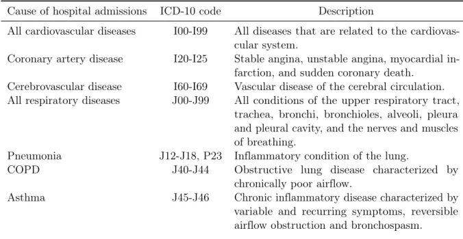
We obtained hospital admission data from the Medical Statistics of the Hospitals maintained by the FSO (2016b). These data are collected by the Swiss cantons and include a wide array of information on people that are admitted to the hospital. Since 1998, Swiss hospitals are obliged by the federal law to submit patient-level data. According to the FSO, the dataset covers 99.9 percent of hospital admissions. Because the quality of data is restricted before 2001, we drop earlier years and focus on patients who were stationary treated in the period 2001 to 2013. Following Schlenker and Walker (2016), we select patients based on their main and secondary diagnosis and include both emergency and elective admissions. The causes of hospital admissions considered in this analysis are listed in Table 2. The table provides information on the cause of hospital admissions, the relevant ICD-10 codes, and a brief description of each cause of hospital admission. We select these causes based on the extensive literature review in WHO (2005) and European Environmental Agency (2015). Therefore, we focus on hospital admissions for cardiovascular and respiratory diseases. We also look at more disaggregated causes of hospital admissions, allowing for a better understanding of the disease-specific treatment effects. To ensure the validity of our identification strategy, we include several negative control outcomes which are specified in Table A5 in the online supplementary materials.

2.3 Control variables

The relationship between ambient air pollution and hospital admissions may be confounded by factors that vary across MedStat regions over time. Among others, such factors are population characteristics, economic conditions and access to outpatient and hospital care facilities.6 _{To account for population}

characteristics, we use registry information from the FSO. We compute a measure of population size to capture changes in the demand for hospital care that are unrelated to changes in pollution exposure. We also consider the share of foreigners, the share of females, and the share of the working-age population in the total population. These variables are supposed to account for migration patterns and the effect of age and gender composition on hospital admissions. Moreover, we include a number of economic covariates: the average household income, an income equality measure, and the unemployment rate. Household income and inequality data are obtained from the Swiss Federal Tax Administration (FTA), and unemployment data from the Swiss State Secretariat for Economic Affairs (SECO). These variables are supposed to capture changes in the financial abilities of the population. Finally, we account for access to outpatient care with a measure of the number of ambulatory doctors, and for access to hospital care

6 _{As for possible border effects, note that the dispersion model already accounts for these effects by}

with a measure of the number of stationary doctors.7

Some additional factors may complicate the identification of the relationship between ambient air pollution and hospital admissions. On the one hand, people living in regions with poor air quality may have a worse health status for reasons that are unrelated to ambient air pollution. For instance, accessing preventive medical care services can be more difficult in certain regions. This could induce a systematic bias in the parameter estimates. On the other hand, people may live in regions with good air quality because they derive utility from unobserved location characteristics that are confounded with air quality. Among others, such characteristics are the availability of recreational infrastructure and a lower density of commercial and industrial infrastructure. When these factors are not accurately taken into account, we could obtain spuriously large estimates of the air pollution effect on hospital admissions. Given our limited knowledge of factors affecting the selection of people into certain geographical locations, standard ordinary least squares (OLS) estimates are likely biased. The potential for selection bias calls for an identification strategy that captures the influence of confounding factors.

3. Empirical approach

To account for unobserved factors, we exploit the panel structure of our data and include both location and time fixed effects in the following count model:8

admit= exp(αi+ Pitβp+ Xitγx+ δt)ηit, (2)

where i is the MedStat region and t is the year. We denote the location fixed effects by αi, and time

fixed effects by δt. These variables are supposed to account for the influence of unobserved confounding

factors. The location fixed effects address unobserved heterogeneity between MedStat regions. Xit is

the matrix of covariates that vary at the region level over time, and ηitis the multiplicative error term.

The treatment variable are summarized by the matrix Pit, measuring the average pollution exposure for

PM10, NO2, SO2, and O3, and the key parameters of interest are βp. These parameters are supposed to

measure the effect of ambient air pollution on hospital admissions.

We consider two model specifications to address unobserved heterogeneity over time. Our baseline specification includes common time fixed effects, whereas our preferred specification includes canton-time

7 _{Ideally, we would account for access to hospital care with a measure of distance to the nearest hospital.}

However, such data are not available for the entire study period.

8 _{Another approach would be to include spatial effects in the regression model. For this reason, we also}

estimate spatial lag panel models for count data (see e.g., Cameron and Trivedi, 2013). The spatial estimates are very similar to the results of our main model and indicate that spatial lags are of minor relevance for most causes of hospital admissions when using the dispersion model pollution measures.

fixed effects.9 _{We prefer the specification with flexible time fixed effects because the Swiss cantons}

have some autonomy in designing health policy instruments. In this way, we can account for shocks generated by cantonal health policies.10 _{Moreover, the canton-time fixed effects are supposed to control}

for other time-variant factors, such as the progression of diseases, that are predictive of the outcome and correlated with the treatment. Among others, such unobserved variables are the relocation of sicker people into areas with better air quality and the access to transport facilities. Ideally, we would like to track people over time and space to explore the temporal component of pollution exposure and, therefore, account for the possible progression of diseases. However, such detailed information is not available for the Swiss population. In any case, the location and canton-time effects should allow us to circumvent the endogeneity problem. Furthermore, we can exclude that sick people are more likely to move because of easier hospital admissions since waiting times in Switzerland are generally absent.

Following Schlenker and Walker (2016), the outcome variable in our regression model is denoted by admit,

representing the non-negative integer count of hospital admissions.11 _{One might transform the outcome}

variable and then estimate the relationship using a linear regression model. Although this approach is practicable for particular types of data, it is inappropriate when the outcome is a count. As discussed in Wooldridge (1999), the linear regression model does not ensure positivity for the predicted values of the count outcome. Moreover, the discrete nature of the count outcome makes it difficult to find a transformation with a conditional mean that is linear in parameters. Finding such a transformation is a particular problem in the presence of heteroskedasticity as the transformed errors would be correlated with the covariates, leading to inconsistent estimates of the treatment effect. Even when the transformation of the conditional mean is correctly specified, it would be impossible to measure the relationship of primary interest. Hence, we model the relationship between the health outcome and the covariates directly, using the exponential form to ensure positivity for the covariates as shown in Equation 2. An advantage of the exponential form is that the response variable can follow different distributional assumptions.

To explore the relationship between ambient air pollution and hospital admissions, we use the Poisson pseudo-maximum likelihood (PML) estimator (Gong and Samaniego, 1981; Gourieroux et al., 1984). The Poisson PML estimator is consistent in the presence of heteroskedasticity, and even if the conditional variance is not proportional to the conditional mean, the Poisson PML estimator is consistent (Wooldridge,

9 _{Switzerland is a federal state of 26 cantons. Each canton has its own constitution, legislature, and}

government. Among others, the cantons are responsible for healthcare services, welfare, law enforcement and public education.

10_{For instance, Switzerland has recently introduced a new hospital financing system to promote}

cost-effective health care. Although the system was simultaneously introduced in all cantons, the reimburse-ment rates for medical treatreimburse-ment are different between cantons.

11_{We are aware that several studies in the health economics literature use admissions per population as}

the outcome variable. However, the absolute number of admissions is more appropriate in this context because we can use a count-data model that reflects the data generating process of hospital admissions due to pollution exposure.

1999; Cameron and Trivedi, 2013). Because the Poisson PML estimator makes no assumption on the dispersion of the fitted values, we do not need to test for this aspect. An advantage of the Poisson PML estimator is that the scale of the dependent variable has no effect on the parameter estimates, which is a challenge for the Negative Binomial PML estimator. Moreover, as long as the conditional mean is correctly specified, the Poisson PML estimator yields estimates that are similar in size to the estimates of both the Gaussian and Negative Binomial PML estimators. To ensure that the distributional assumption has no impact on the parameter estimates, we also estimate Equation 2 using these alternative PML estimators (see the online supplementary materials). Lastly, to address heteroskedasticity in the error term, we use a robust variance estimator and account for clustering at the MedStat region level (Cameron and Miller, 2015).

4. Results

We first explore the relationship between ambient air pollution and hospital admissions with the baseline specification; then we extend the analysis by comparing the effect of different distributional assumptions and testing for non-linearity in the treatment effect. Finally, we conduct falsification tests to ensure the robustness of our identification strategy.

4.1 The effect of ambient air pollution on hospital admissions

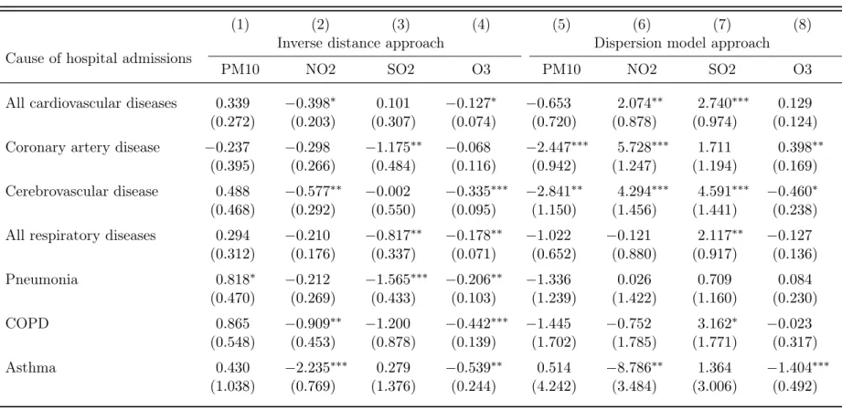
We commence our empirical analysis by exploring the relationship between ambient air pollution and hospital admissions in the general population. Table 3 summarizes the Poisson PML estimates for the investigated causes of hospital admission. All specifications include covariates and fixed effects for MedStat regions and time.12 _{We report the estimates of the treatment effect measuring the air pollution}

using the inverse distance approach in columns 1-4, and the dispersion model approach in columns 5-8.13

As suggested earlier, our regression results could indicate an endogeneity problem for the inverse distance approach as most estimates have a negative sign or are not statistically significant at the 10 percent confidence level.14 _{This problem is the primary concern of our analysis and the reason why we advance}

the use of a dispersion model approach to solve the endogeneity issue. Therefore, the remaining discussion is solely concerned with the parameter estimates of the dispersion model approach as these estimates are likely less affected by measurement bias.15

12_{We do not report the estimates of the control variables because of space limitations. The table shows}

the estimates of 14 (7x2) regressions. The estimates including all covariates are available upon request from the authors.

13_{Note that the effects of different pollutants are comparable since they are all measured in µg/m}3_. 14_{The negative parameter estimates for some types of pollution could also be caused by insufficient}

variation in the measures of exposure. For instance, since there are only a few SO2 monitoring sites, the within variation in pollution exposure is limited, inducing collinearity between the fixed effects and the measures of pollution exposure.

15_{As discussed in the literature, in this case the measurement error is likely non-classical. This implies}

The Poisson PML estimates based on the dispersion model approach explain between 80 and 91 percent of the variation, and the pollution measures account for 2.4 to 10.1 percent of the overall variation in hospitalization data.16 _{The estimates provide evidence for a significant association between ambient air}

pollution and hospital admissions for cardiovascular diseases, but only weak evidence for respiratory diseases. Except for PM10 exposure and hospital admissions for asthma, all estimates for respiratory diseases are not statistically significant. As for cardiovascular diseases, the strongest association with pollution is found for SO2, for which a 1 unit increase in pollution exposure is associated with a 2.6 percent increase in the incidence of hospital admissions for coronary artery diseases. This implies that an increase in SO2 exposure by one standard deviation increases hospitalizations by more than 2.2 patients. Although only some of the estimates for O3 exposure are statistically significant, the treatment effect is in general much smaller than for PM10, NO2 and SO2.

Even though our baseline specification with MedStat region and time fixed effects provides evidence for a positive association between some ambient air pollutants and hospital admissions for cardiovascular diseases, it is possible that unobserved location characteristics varying between cantons and over time are correlated with the measures of air pollution. To account for these factors, we allow the time fixed effects to be flexible and estimate Equation 2 with canton-time fixed effects. The regression results are provided in Table 4. Again, we compare the estimates using the inverse distance approach with the estimates of the dispersion model approach. The negative and partially significant estimates for the inverse distance approach provide further evidence of a possible endogeneity issue. Conversely, the estimates for the dispersion model approach generally show the expected sign and are statistically significant.

The difference in parameter estimates for the IDW approach and the dispersion model is likely due to the inability of the IDW approach to account for different emission sources, such as road traffic and industrial and commercial activities, as well as the atmospheric conditions, which include wind speed and direction, air temperature and mixing height. For instance, in the Southern part of Switzerland, where the mountains channel the wind, the Alpine topography has a significant impact on the distribution of pollutants. Most monitoring sites in this area are in the central valleys (see Figure A1 for the distribution map), where North is the primary wind direction. Since the IDW approach is unable to account for these characteristics of pollutant dispersion, the method suffers from an endogeneity issue that is systematic but likely not normally distributed. This type of measurement error is not easily resolvable with econometric methods and implies that finding insignificant and biased treatment estimates is not surprising.

We now turn to the discussion of our estimates in details. The results of the dispersion model approach indicate that PM10 exposure has no statistically significant effect on hospital admissions for cardiovascular and respiratory diseases in Switzerland. One possible reason for this results is that PM10 levels in

16_{As a measure of explanatory power, we use the Pseudo R-squared value, which is defined as the squared}

Switzerland are lower than in other developed countries. Another reason is that the inclusion of time and canton-time fixed effects is capturing the impact of PM10 levels that steadily decreased in the last two decades. Therefore, we cannot conclude that current PM10 exposure does not affect hospital admissions. Conversely, the estimates of the treatment effect for NO2 and SO2 indicate a positive association between pollution exposure and hospital admissions, as suggested by some recent studies (César et al., 2015; Dehbi et al., 2017; Newell et al., 2018). Both pollutants have statistically significant and economically meaningful effects on hospital admissions for cardiovascular diseases. The treatment effect is overall larger for SO2 than for NO2. We find that the incidence of hospital admissions for cardiovascular diseases is 1.5 percent higher for NO2, and 2.8 percent higher for SO2, when the pollutant exposure increases by 1 unit. This implies that a one-standard deviation increase of pollution exposure results in an increase of hospitalization by 18.7 patients for NO2 and by 8.7 patients for SO2, respectively. The SO2 effect on hospital admissions for respiratory diseases is smaller with the incidence rate increasing most for chronic obstructive pulmonary diseases (COPD). Moreover, we find no evidence for a statistically significant association between pollution exposure and hospital admissions for asthma. The last column of Table 4 reports the parameter estimates for O3. We find no evidence for a significant effect of O3 exposure on hospital admissions, which is likely because summer spikes are captured insufficiently by our annual pollution measure.

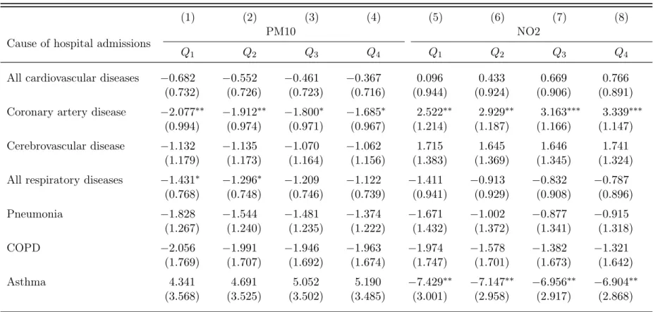
To ensure the validity of our baseline estimation results, we conducted two robustness checks of our statistical approach. First, we extended the analysis by comparing the effect of different distributional assumptions. The estimates of the treatment effect for the Gaussian and the Negative Binomial PML estimators are provided in the online supplementary materials (Tables A1 and A2). We find that all estimates are similar to the estimates for the Poisson distribution regarding the significance level, but are larger regarding the size of the treatment effect. Second, we account for the potential effect of non-linearity in the treatment effect. We classify each treatment variable for the dispersion model approach into quartiles and interact the quartile dummies with the treatment measure. We find no compelling evidence for non-linearity in the PM10 treatment effect (see Tables A3 and A4 in the online supplementary materials). The Poisson PML estimates confirm that PM10 exposure has no statistically significant effect on hospital admissions in Switzerland. Additionally, the quartile regression results indicate that both NO2 and SO2 have statistically significant effects on hospital admissions. We find no evidence for non-linearity in the treatment effect for NO2, and only limited evidence for SO2. Overall, the largest estimates are observed for the last quartile. The estimation results for O3 are similar to those presented in our main regression table, providing no evidence for a statistically significant treatment effect. 4.2 Falsification tests

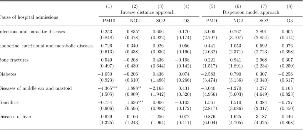
To provide further support for the robustness of our identification strategy and our claim that the dispersion model approach allows for more accurate identification of the pollution treatment effects, we

conducted a couple of negative control falsification tests. For this purpose, we randomly selected diagnoses at different ICD-10 levels excluding diagnoses considered in the baseline selection. These diagnoses are listed in Table A5 of the online supplementary materials. We estimated the relationship for the preferred specification with MedStat region and canton-time fixed effects.

The estimation results are summarized in Table 5. Again, we observe that the dispersion model approach outperforms the inverse distance approach. Indeed, while we find no evidence for a statistically significant relationship between pollution exposure and the negative control outcomes in the dispersion model approach, the inverse distance approach shows statistically significant evidence (positive or negative).

5. Conclusions

Ambient air pollution is the environmental factor with the greatest impact on human health. Several epidemiological studies provide evidence for a significant association between ambient air pollution and human health. However, the recent economic literature has challenged the identification strategy used in these studies. This paper explores the association between ambient air pollution and morbidity using hospital admission data from Switzerland. We try to strengthen the understanding of the impact of air pollutants on morbidity using geographically explicit air pollution measures derived from a dispersion model. This novel approach enables us to circumvent the measurement problem at the source and to construct a reliable measure of local pollution exposure.

We find a significant association between ambient air pollution and health outcomes, and these results are robust to different distributional assumptions and non-linearity in the treatment effect. We also find substantial differences among causes of hospital admission. While SO2 and NO2 exposure appear to be significantly associated with admission rates for coronary artery and cerebrovascular diseases, the association between PM10 exposure and hospital admissions is not confirmed in all model specifications. The limited statistical evidence on the impact of PM10 exposure may be due to the low levels of pollution in Switzerland, or to the econometric specification that include time and canton-time fixed effects capturing the steadily decrease of this pollutant in the last decades.

Our results show that the inverse distance approach (IDW), which is the conventional approach to measure air pollution in previous studies, is likely to induce systematic estimation bias. In contrast, the dispersion model approach seems to be able to address the endogeneity problem related to the measurement of local pollutant exposure. Still, some of the emission sources and process characteristics used in the dispersion model could be subject to imprecise measurement. For instance, the amount of pollution from the use of vehicles is estimated using road usage inventories instead of actual road usage.

Although exposure to air pollution has decreased significantly during the study period, our findings may indicate that there is still potential to further reduce the exposure to pollutants with the aim to mitigate the negative impact on health outcomes. Thus, our results may contribute to a more accurate

evaluation of future environmental policies aiming at a reduction of air pollution exposure. For instance, effort should focus on reducing the exposure to SO2 and NO2, which show the strongest association with hospital admissions, to provide the largest benefits for human health.

References

Beatty, T. K. and Shimshack, J. P. 2014. Air pollution and children’s respiratory health: A cohort analysis. Journal of Environmental Economics and Management 67(1), 39–57.

Bound, J. and Krueger, A. B. 1991. The Extent of Measurement Error in Longitudinal Earnings Data: Do Two Wrongs Make a Right?. Journal of Labor Economics 9(1), 1–24.

Cameron, C. and Miller, D. 2015. A practitioner’s guide to cluster-robust inference. Journal of Human Resources 50(2), 317–372.

Cameron, C. and Trivedi, P. 2013. Regression Analysis of Count Data. Cambridge: Cambridge University Press.

Chay, K. Y. and Greenstone, M. 2003. The impact of air pollution on infant mortality: Evidence from geographic variation in pollution shocks induced by a recession. The Quarterly Journal of Economics 118(3), 1121–1167.

Currie, J. and Neidell, M. 2005. Air pollution and infant health: What can we learn from California’s recent experience?. The Quarterly Journal of Economics 120(3), 1003–1030.

Currie, J., Neidell, M. and Schmieder, J. F. 2009. Air pollution and infant health: Lessons from New Jersey. Journal of Health Economics 28(3), 688–703.

Deryugina, T., Heutel, G., Miller, N., Molitor, D. and Reif, J. 2016. The mortality and medical costs of air pollution: Evidence from changes in wind direction. NBER Working Paper 22796 .

European Environmental Agency 2015. Air Quality in Europe – 2015 Report. Luxembourg: Publication Office of the European Union.

Federal Council 2016. Ordinance on air pollution control. https://www.admin.ch/ opc/en/classified-compilation/19850321/index.html (access date: 11/15/2016).

FOEN 2016. Air pollution maps. http://www.bafu.admin.ch/luft/luftbelastung/schadstoff karten (access date: 11/15/2016).

FSO 2016a. Area statistics. https://www.bfs.admin.ch/bfs/de/home/statistiken/raum-umwelt/erhebungen/area.html(access date: 11/15/2016).

FSO 2016b. Medical statistics of the hospitals. https://www.bfs.admin.ch/bfs/de/home/sta tis-tiken/gesundheit/erhebungen/ms.html (access date: 11/15/2016).

Gong, G. and Samaniego, F. J. 1981. Pseudo maximum likelihood estimation: Theory and applications. Annals of Statistics 9(4), 861–869.

Gourieroux, C., Monfort, A. and Trognon, A. 1984. Pseudo maximum likelihood methods: Applications to poisson models. Econometrica 52(3), 701–720.

He, G., Fan, M. and Zhou, M. 2016. The effect of air pollution on mortality in China: Evidence from the 2008 Beijing Olympic Games. Journal of Environmental Economics and Management 79, 18–39. Heldstab, J., Leippert, F., Wüthrich, P., Künzli, T. and Stampfli, M. 2013. PM10 and PM2.5 ambient

concentrations in Switzerland. Bern: FOEN.

Knittel, C. R., Miller, D. L. and Sanders, N. J. 2016. Caution, drivers! children present: Traffic, pollution, and infant health. Review of Economics and Statistics 98(2), 350–366.

Lagravinese, R., Moscone, F., Tosetti, E. and Lee, H. 2014. The impact of air pollution on hospital admissions: Evidence from Italy. Regional Science and Urban Economics 49, 278–285.

Luechinger, S. 2014. Air pollution and infant mortality: A natural experiment from power plant desulfur-ization. Journal of Health Economics 37, 219–231.

Moretti, R. and Neidell, M. 2011. Pollution, health, and avoidance behavior evidence from the ports of los angeles. Journal of Human Resources 46(1), 154–175.

Sanders, N. J. and Stoecker, C. 2015. Where have all the young men gone? Using sex ratios to measure fetal death rates. Journal of Health Economics 41, 30–45.

Schlenker, W. and Walker, W. R. 2016. Airports, air pollution, and contemporaneous health. The Review of Economic Studies 83(2), 768–809.

WHO 2005. Air Quality Guidelines: Particulate Matter, Ozone, Nitrogen Dioxide and Sulfur Dioxide. Copenhagen: WHO Regional Office for Europe.

WHO Regional Office for Europe and OECD 2015. Economic Cost of the Health Impact of Air Pollution in Europe: Clean Air, Health and Wealth. Copenhagen: WHO Regional Office for Europe.

Wooldridge, J. 1999. Handbook of Applied Econometrics Volume II: Quasi-Likelihood Methods for Count Data. Oxford: Blackwell Publishing Inc.

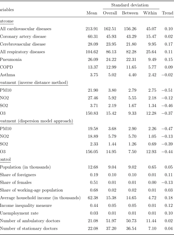
Table 1: Descriptive statistics of outcome, treatment and control variables

Variables

Standard deviation

Mean Overall Between Within Trend Outcome

All cardiovascular diseases 213.91 162.51 156.26 45.07 0.10

Coronary artery disease 60.31 45.93 43.29 15.47 0.02

Cerebrovascular disease 28.09 23.95 21.80 9.95 0.17

All respiratory diseases 104.62 86.13 82.28 25.64 0.11

Pneumonia 26.09 24.22 22.31 9.49 0.15

COPD 13.37 12.99 11.65 5.77 0.09

Asthma 3.75 5.02 4.40 2.42 −0.02

Treatment (inverse distance method)

PM10 21.90 3.80 2.79 2.75 −0.51

NO2 27.46 5.92 5.55 2.18 −0.12

SO2 3.71 2.19 1.67 1.34 −0.46

O3 150.83 15.42 9.33 12.28 −0.37

Treatment (dispersion model approach)

PM10 19.58 3.68 2.90 2.26 −0.47

NO2 18.89 5.79 5.70 1.05 −0.13

SO2 2.33 1.44 1.26 0.69 −0.39

O3 156.05 14.95 7.50 12.93 −0.44

Control

Population (in thousands) 12.68 9.04 9.02 0.65 0.05

Share of foreigners 0.19 0.10 0.10 0.01 0.11

Share of females 0.51 0.01 0.01 0.00 −0.13

Share of working-age population 0.68 0.02 0.02 0.01 0.03

Average household income (in thousands) 62.38 15.38 14.65 4.72 0.18

Income inequality measure 0.44 0.05 0.05 0.01 0.12

Unemployment rate 0.03 0.01 0.01 0.01 0.10

Number of ambulatory doctors 21.08 51.97 50.73 11.44 0.02

Number of stationary doctors 22.08 37.20 36.54 7.10 0.04

Note: This table summarizes statistics for outcome, treatment and control variables. The statistics is based on data for 604 MedStat regions and the period 2001 to 2013. We present the mean, and the standard deviation in terms of overall, between and within variation, and the time trend. The time trend is defined as the correlation between each variable and time.

Table 2: Investigated causes of hospital admissions

Cause of hospital admissions

ICD-10 code

Description

All cardiovascular diseases

I00-I99

All diseases that are related to the

cardiovas-cular system.

Coronary artery disease

I20-I25

Stable angina, unstable angina, myocardial

in-farction, and sudden coronary death.

Cerebrovascular disease

I60-I69

Vascular disease of the cerebral circulation.

All respiratory diseases

J00-J99

All conditions of the upper respiratory tract,

trachea, bronchi, bronchioles, alveoli, pleura

and pleural cavity, and the nerves and muscles

of breathing.

Pneumonia

J12-J18, P23

Inflammatory condition of the lung.

COPD

J40-J44

Obstructive lung disease characterized by

chronically poor airflow.

Asthma

J45-J46

Chronic inflammatory disease characterized by

variable and recurring symptoms, reversible

airflow obstruction and bronchospasm.

Table 3: Baseline specification with MedStat region and time fixed effects (Poisson PML estimates)

(1)

(2)

(3)

(4)

(5)

(6)

(7)

(8)

Cause of hospital admissions

Inverse distance approach

Dispersion model approach

PM10

NO2

SO2

O3

PM10

NO2

SO2

O3

All cardiovascular diseases

0.526

−0.325

−0.186

−0.014

0.775

1.235

0.709

0.140

(0.186)

(0.118)

(0.300)

(0.036)

(0.601)

(0.817)

(0.648)

(0.072)

Coronary artery disease

0.843

−0.531

_−0.949

_−0.085

_0.712

_1.834

_2.567

_0.134

(0.225)

(0.159)

(0.445)

(0.050)

(0.695)

(0.929)

(0.856)

(0.086)

Cerebrovascular disease

0.320

−0.291

0.195

0.010

−0.047

2.197

0.814

0.247

(0.325)

(0.204)

(0.401)

(0.061)

(0.914)

(1.130)

(0.797)

(0.114)

All respiratory diseases

0.320

0.099

−0.566

−0.124

0.826

−1.001

−0.360

0.094

(0.275)

(0.161)

(0.297)

(0.043)

(0.635)

(0.772)

(0.636)

(0.072)

Pneumonia

0.342

0.075

−1.160

−0.079

0.171

−0.258

−1.564

0.151

(0.289)

(0.184)

(0.347)

(0.056)

(0.817)

(0.971)

(0.833)

(0.092)

COPD

0.306

−0.230

−2.127

_−0.234

_−1.151

_−0.884

_−0.545

_0.160

(0.426)

(0.269)

(0.644)

(0.088)

(1.082)

(1.222)

(1.084)

(0.133)

Asthma

2.070

−1.010

_−0.861

_−0.804

_6.050

_−0.049

_−1.781

_−0.632

(0.635)

(0.390)

(0.779)

(0.135)

(1.519)

(1.334)

(1.684)

(0.186)

Note: This table reports the joint estimates of the treatment effect of pollutants on different causes of hospital admissions. All estimates and standard errors are rescaled (x100). The sample consists of 604 MedStat regions for the period 2001 to 2013. We assume that the data generating process follows a Poisson distribution. All regressions include control variables and both year and MedStat region fixed effects. Columns 1-4 report the estimates of the treatment effect by pollutant for the inverse distance approach, and columns 5-8 the results for the dispersion model approach. The heteroscedasticity-robust standard errors are provided in parenthesis, and are adjusted for within cluster correlation at the MedStat region level. ∗∗∗_, ∗∗_{, and}∗ _{indicate significance at the 1 percent, 5 percent, and 10 percent, respectively.}

Table 4: Preferred specification with MedStat region and canton-time fixed effects (Poisson PML estimates)

(1)

(2)

(3)

(4)

(5)

(6)

(7)

(8)

Cause of hospital admissions

Inverse distance approach

Dispersion model approach

PM10

NO2

SO2

O3

PM10

NO2

SO2

O3

All cardiovascular diseases

0.403

−0.310

−0.051

−0.134

−0.175

1.506

2.827

0.036

(0.205)

(0.176)

(0.265)

(0.059)

(0.718)

(0.868)

(0.864)

(0.099)

Coronary artery disease

0.354

−0.364

−1.089

_−0.180

_−1.185

_4.327

_2.017

_0.143

(0.305)

(0.244)

(0.384)

(0.091)

(0.958)

(1.123)

(0.988)

(0.148)

Cerebrovascular disease

0.400

−0.565

−0.476

−0.178

−1.562

2.394

3.834

−0.120

(0.347)

(0.235)

(0.427)

(0.077)

(1.154)

(1.272)

(1.253)

(0.196)

All respiratory diseases

−0.135

0.187

−0.381

−0.177

−1.024

−0.201

2.301

−0.078

(0.266)

(0.169)

(0.330)

(0.065)

(0.728)

(0.880)

(0.893)

(0.110)

Pneumonia

0.622

−0.024

−1.571

−0.181

−1.444

0.123

0.639

0.010

(0.367)

(0.235)

(0.431)

(0.085)

(1.189)

(1.273)

(1.066)

(0.178)

COPD

0.031

−0.424

−1.600

_−0.387

_−2.470

_−0.587

_2.143

_0.015

(0.537)

(0.403)

(0.775)

(0.134)

(1.628)

(1.651)

(1.577)

(0.263)

Asthma

2.024

−1.384

_−1.020

_−0.317

_5.237

_−5.737

_2.559

_−0.202

(0.843)

(0.633)

(1.087)

(0.207)

(3.385)

(2.780)

(2.544)

(0.413)

Note: This table reports the joint estimates of the treatment effect of pollutants on different causes of hospital admissions. All estimates and standard errors are rescaled (x100). The sample consists of 604 MedStat regions for the period 2001 to 2013. We assume that the data generating process follows a Poisson distribution. All regressions include control variables and both canton-year and MedStat region fixed effects. Columns 1-4 report the estimates of the treatment effect by pollutant for the inverse distance approach, and columns 5-8 the results for the dispersion model approach. The heteroscedasticity-robust standard errors are provided in parenthesis, and are adjusted for within cluster correlation at the MedStat region level. ∗∗∗_, ∗∗_{, and}∗ _{indicate significance at the 1 percent, 5 percent, and 10 percent, respectively.}

Table 5: Falsification tests for preferred specification with MedStat region and canton-time fixed effects (Poisson PML estimates)

(1)

(2)

(3)

(4)

(5)

(6)

(7)

(8)

Cause of hospital admissions

Inverse distance approach

Dispersion model approach

PM10

NO2

SO2

O3

PM10

NO2

SO2

O3

Infectious and parasitic diseases

0.253

−0.835

0.606

−0.170

3.005

−0.767

2.891

0.005

(0.848)

(0.478)

(0.922)

(0.174)

(2.797)

(3.107)

(2.854)

(0.414)

Endocrine, nutritional and metabolic diseases −0.726

−0.340

0.926

0.056

−0.441

1.053

0.592

0.076

(0.613)

(0.438)

(0.936)

(0.166)

(2.632)

(2.371)

(2.723)

(0.398)

Bone fractures

0.549

−0.208

0.436

−0.168

0.221

0.941

2.968

0.307

(0.497)

(0.430)

(0.644)

(0.142)

(1.517)

(1.891)

(2.234)

(0.250)

Diabetes

−1.050

−0.206

0.436

0.074

−2.583

0.790

0.307

−0.256

(0.923)

(0.610)

(1.486)

(0.266)

(3.474)

(3.136)

(3.340)

(0.617)

Diseases of middle ear and mastoid

−4.365

1.888

−2.168

0.431

−3.040

−1.270

1.277

0.163

(1.505)

(0.909)

(1.942)

(0.320)

(4.956)

(5.603)

(4.649)

(0.823)

Tonsillitis

−0.754

1.636

0.006

−0.103

1.561

1.510

0.384

−0.727

(0.906)

(0.596)

(0.982)

(0.172)

(2.817)

(3.086)

(2.317)

(0.450)

Diseases of liver

0.929

−0.166

−1.256

−0.072

0.876

1.625

3.187

−0.446

(1.325)

(1.243)

(1.964)

(0.411)

(6.004)

(4.705)

(4.425)

(0.868)

Note: This table reports the joint estimates of the treatment effect of pollutants on different causes of hospital admissions. All estimates and standard errors are rescaled (x100). The sample consists of 604 MedStat regions for the period 2001 to 2013. We assume that the data generating process follows a Poisson distribution. All regressions include control variables and both canton-year and MedStat region fixed effects. Columns 1-4 report the estimates of the treatment effect by pollutant for the inverse distance approach, and columns 5-8 the results for the dispersion model approach. The heteroscedasticity-robust standard errors are provided in parenthesis, and are adjusted for within cluster correlation at the MedStat region level. ∗∗∗_, ∗∗_{, and}∗ _{indicate significance at the 1}

percent, 5 percent, and 10 percent, respectively.

PM10 NO2

SO2 O3

(1) (2) (3) (4) (5) (6) (7) (8) (9) (10)

(1) (2) (3) (4) (5) (6) (7) (8) (9) (10)

Figure 1: Between variation in pollution exposure averaged for the period 2001 to 2013.

Note: The four maps show the average daily pollution exposure by MedStat region. The dark green color (1) indicates the lowest level whereas

PM10 NO2

SO2 O3

(1) (2) (3) (4) (5) (6) (7) (8) (9) (10)

(1) (2) (3) (4) (5) (6) (7) (8) (9) (10)

Figure 2: Within variation in pollution exposure for the period 2001 to 2013.

Note: The four maps show the within variation of average daily pollution exposure by MedStat region. The dark green color (1) indicates the

Online supplementary materials

Table A1: The effect of ambient air pollution on hospital admissions (Gaussian PML estimates)

Table A2: The effect of ambient air pollution on hospital admissions (Negative Binomial PML estimates) Table A3: Non-linearity in the pollution treatment effects (Poisson PML estimates)

Table A4: Non-linearity in the pollution treatment effects (Poisson PML estimates) Table A5: Investigated causes of hospital admissions for falsification tests

Figure A1: Geographical distribution of pollution monitoring sites (red bullets) in the 604 MedStat regions during the period 2001 to 2013.

Table A1: The effect of ambient air pollution on hospital admissions (Gaussian PML estimates)

(1)

(2)

(3)

(4)

(5)

(6)

(7)

(8)

Cause of hospital admissions

Inverse distance approach

Dispersion model approach

PM10

NO2

SO2

O3

PM10

NO2

SO2

O3

All cardiovascular diseases

0.339

−0.398

0.101

−0.127

−0.653

2.074

2.740

0.129

(0.272)

(0.203)

(0.307)

(0.074)

(0.720)

(0.878)

(0.974)

(0.124)

Coronary artery disease

−0.237

−0.298

−1.175

_−0.068

_−2.447

_5.728

_1.711

_0.398

(0.395)

(0.266)

(0.484)

(0.116)

(0.942)

(1.247)

(1.194)

(0.169)

Cerebrovascular disease

0.488

−0.577

−0.002

−0.335

−2.841

4.294

4.591

−0.460

(0.468)

(0.292)

(0.550)

(0.095)

(1.150)

(1.456)

(1.441)

(0.238)

All respiratory diseases

0.294

−0.210

−0.817

−0.178

−1.022

−0.121

2.117

−0.127

(0.312)

(0.176)

(0.337)

(0.071)

(0.652)

(0.880)

(0.917)

(0.136)

Pneumonia

0.818

−0.212

−1.565

−0.206

−1.336

0.026

0.709

0.084

(0.470)

(0.269)

(0.433)

(0.103)

(1.239)

(1.422)

(1.160)

(0.230)

COPD

0.865

−0.909

_−1.200

_−0.442

_−1.445

_−0.752

_3.162

_−0.023

(0.548)

(0.453)

(0.878)

(0.139)

(1.702)

(1.785)

(1.771)

(0.317)

Asthma

0.430

−2.235

_0.279

_−0.539

_0.514

_−8.786

_1.364

_−1.404

(1.038)

(0.769)

(1.376)

(0.244)

(4.242)

(3.484)

(3.006)

(0.492)

Note: This table reports the joint estimates of the treatment effect of pollutants for the Gaussian PML estimator on different causes of hospital admissions. All estimates and standard errors are rescaled (x100). The sample consists of 604 MedStat regions for the period 2001 to 2013. All regressions include control variables and both year-by-canton and MedStat region fixed effects. Columns 1-4 report the estimates of the treatment effect by pollutant for the inverse distance approach, and columns 5-8 the results for the dispersion model approach. The heteroscedasticity-robust standard errors are provided in parenthesis, and are adjusted for within cluster correlation at the MedStat region level. ∗∗∗_,∗∗_{, and}∗ _{indicate significance at the 1 percent, 5 percent, and 10 percent, respectively.}

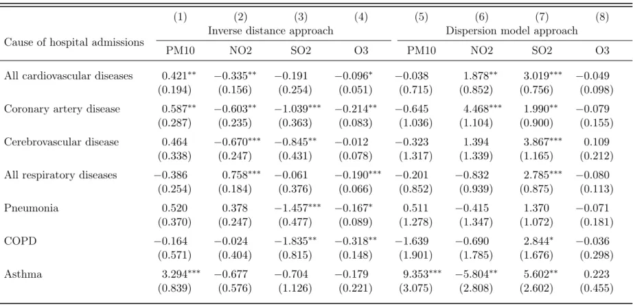
Table A2: The effect of ambient air pollution on hospital admissions (Negative Binomial PML estimates)

(1)

(2)

(3)

(4)

(5)

(6)

(7)

(8)

Cause of hospital admissions

Inverse distance approach

Dispersion model approach

PM10

NO2

SO2

O3

PM10

NO2

SO2

O3

All cardiovascular diseases

0.421

−0.335

−0.191

−0.096

−0.038

1.878

3.019

−0.049

(0.194)

(0.156)

(0.254)

(0.051)

(0.715)

(0.852)

(0.756)

(0.098)

Coronary artery disease

0.587

−0.603

_−1.039

_−0.214

_−0.645

_4.468

_1.990

_−0.079

(0.287)

(0.235)

(0.363)

(0.083)

(1.036)

(1.104)

(0.900)

(0.155)

Cerebrovascular disease

0.464

−0.670

−0.845

−0.012

−0.323

1.394

3.867

0.109

(0.338)

(0.247)

(0.431)

(0.078)

(1.317)

(1.339)

(1.165)

(0.212)

All respiratory diseases

−0.386

0.758

−0.061

−0.190

−0.201

−0.832

2.785

−0.080

(0.254)

(0.184)

(0.376)

(0.066)

(0.852)

(0.939)

(0.875)

(0.113)

Pneumonia

0.520

0.378

−1.457

−0.167

0.511

−0.415

1.370

−0.071

(0.370)

(0.247)

(0.477)

(0.089)

(1.278)

(1.347)

(1.072)

(0.181)

COPD

−0.164

−0.024

−1.835

_−0.318

_−1.639

_−0.690

_2.844

_−0.036

(0.571)

(0.404)

(0.815)

(0.148)

(1.901)

(1.785)

(1.676)

(0.298)

Asthma

3.294

−0.677

−0.704

−0.179

9.353

−5.804

_5.602

_0.223

(0.839)

(0.576)

(1.126)

(0.221)

(3.075)

(2.808)

(2.602)

(0.455)

Note: This table reports the joint estimates of the treatment effect of pollutants for the Negative Binomial PML estimator on different causes of hospital admissions. All estimates and standard errors are rescaled (x100). The sample consists of 604 MedStat regions for the period 2001 to 2013. All regressions include control variables and both year-by-canton and MedStat region fixed effects. Columns 1-4 report the estimates of the treatment effect by pollutant for the inverse distance approach, and columns 5-8 the results for the dispersion model approach. The heteroscedasticity-robust standard errors are provided in parenthesis, and are adjusted for within cluster correlation at the MedStat region level. ∗∗∗_,∗∗_{, and}∗ _{indicate significance at the 1 percent, 5 percent, and 10 percent, respectively.}

Table A3: Non-linearity in the pollution treatment effects (Poisson PML estimates)

(1)

(2)

(3)

(4)

(5)

(6)

(7)

(8)

Cause of hospital admissions

PM10

NO2

Q

Q

Q

Q

Q

Q

Q

Q

All cardiovascular diseases

−0.682

−0.552

−0.461

−0.367

0.096

0.433

0.669

0.766

(0.732)

(0.726)

(0.723)

(0.716)

(0.944)

(0.924)

(0.906)

(0.891)

Coronary artery disease

−2.077

_−1.912

_−1.800

_−1.685

_2.522

_2.929

_3.163

_3.339

(0.994)

(0.974)

(0.971)

(0.967)

(1.214)

(1.187)

(1.166)

(1.147)

Cerebrovascular disease

−1.132

−1.135

−1.070

−1.062

1.715

1.645

1.646

1.741

(1.179)

(1.173)

(1.164)

(1.156)

(1.383)

(1.369)

(1.345)

(1.324)

All respiratory diseases

−1.431

−1.296

−1.209

−1.122

−1.411

−0.913

−0.832

−0.787

(0.768)

(0.748)

(0.746)

(0.739)

(0.941)

(0.929)

(0.908)

(0.896)

Pneumonia

−1.828

−1.544

−1.481

−1.374

−1.671

−1.002

−0.877

−0.915

(1.267)

(1.240)

(1.235)

(1.222)

(1.432)

(1.372)

(1.341)

(1.318)

COPD

−2.056

−1.991

−1.946

−1.963

−1.974

−1.578

−1.382

−1.321

(1.769)

(1.707)

(1.692)

(1.674)

(1.747)

(1.701)

(1.673)

(1.642)

Asthma

4.341

4.691

5.052

5.190

−7.429

_−7.147

_−6.956

_−6.904

(3.568)

(3.525)

(3.502)

(3.485)

(3.001)

(2.958)

(2.917)

(2.868)

Note: This table reports the estimates of the treatment effect for the Poisson PML estimator obtained by estimating different models that include quartile pollution measures. All estimates and standard errors are rescaled (x100). The sample consists of 604 MedStat regions for the period 2001 to 2013. All regressions include control variables and both year-by-canton and MedStat region fixed effects. The regression results are sorted by cause of hospital admissions. Columns 1-4 report the estimates of the non-linear treatment effect for PM10, and columns 5-8 the results for NO2. The heteroscedasticity-robust standard errors are provided in parenthesis, and are adjusted for within cluster correlation at the MedStat region level. ∗∗∗_,∗∗_{, and} ∗ _{indicate significance at the 1 percent, 5 percent, and 10 percent, respectively.}