Dynamics of rotors incorporating squeeze film dampers

Dynamics of Rotors Incorporating

Squeeze Film Dampers

by

ALY EL-SHAFEI

B. Mech. Eng., Cairo University (1981) M. Eng., Cairo University (1983)

SUBMITTED TO THE DEPARTMENT OF MECHANICAL ENGINEERING IN PARTIAL FULFILLMENT OF THE REQUIREMENTS FOR THE DEGREE OF

DOCTOR OF PHILOSOPHY

at the

MASSACHUSETTS INSTITUTE OF TECHNOLOGY September (1988)

@ Aly El-Shafei, 1988

The author hereby grants to MIT permission to reproduce and to distribute copies of this

i f& /A

thes document in whole or in part. ignaureof Author....

ignatur

of A u hor...

..

... .. ...

.. . .... .. ...

I ii '

I ...

kStephen H. Crandall Ford Professor of Engineering Thesis Supervisor A ccepted by...r . ... ...

Ain A. Sonin, Chairman

MASSACHUSETTS INSTITUTE Departmental Graduate Committee

OF TE-HWOLOGY

SEP 06 1988

UBMUES

The Libraries

Massachusetts Institute of Technology Cambridge, Massachusetts 02139 Institute Archives and Special Collections

Room 14N-118 (617) 253-5688

This is the most complete text of the

thesis available. The following page(s) were not included in the copy of the

thesis deposited in the Institute Archives

supplemented to account for the kinetic energy of the fluid particles that cross the control surface.

Using the kinetic coenergy method the fluid inertia forces acting in both long and short squeeze film dampers are determined. The inertia characteristics of the dampers are presented and are shown to be nonlinear functions of the amplitude of the journal orbit. It is also shown that the fluid inertia forces predicted by the solution of the Navier-Stokes equations for the case of a small circular-centered whirl is the same as that predicted by the kinetic coenergy method.

Finally this model of squeeze film dampers is incorporated in a dynamic analysis of a Jeffcott rotor incorporating SFDs. The steady state unbalance response of the rotor is obtained, and parametric studies of the system are presented. The nonlinear performance of the system is illustrated by the occurence of the jump phenomenon. It is shown that fluid inertia introduces higher critical speeds and reduces the tendency of the rotors to exhibit the jump phenomenon.

Thesis Supervisor: Professor Stephen H. Crandall Title: Ford Professor of Engineering

Acknowledgments

I am very lucky to have my thesis done under the supervision of Professor Stephen H. Crandall. Not only is he a leader in his scientific and engineering fields, but also he is a sensitive and caring person to whom I am indebted for a lot of the knowledge I gained at M.I.T. I would like to thank Professor Crandall for his guidance, encouragement and supervision.

I also would like to thank the members of my thesis committee: Professors T. R. Akylas, J. Dugundji and J. K. Hedrick. In particular I would like to thank Professors Akylas and Dugundji for several discussions that gave me further insight into the problems at hand. I had also several discussions with Professor P. Leehey, for which I am thankful.

I am indebted to the Egyptian government which provided me with financial support for my studies at M.I.T. In particular, I would like to thank Mr. Adel Abdel Hamid, of the Egyptian Cultural and Educational Bureau in Washington D. C., who

administered my fellowship program.

This thesis was done within the Acoustics and Vibration Laboratory at M.I.T. Over the years, several of my fellow students contributed both to my academic and social lives, for which I would like to thank each and every one of them.

My family has been quite on inspiration. My father, mother, brother and sister provided me with love and support (financial and otherwise). My loving wife had to endure my often irregular study schedule, and she brought to life our little precious Ahmed. To all of them this thesis is dedicated.

Contents

1.3 Thesis goals and outline

Chapter 2 Damping forces in squeeze film dampers 2.1 Reynolds equation

2.2 Short bearing approximation 2.3 Long bearing approximation 2.4 Fluid inertia

Chapter 3 Fluid inertia effects in squeezing flows

3.1 Poiseuille flow resulting from squeezing motion 3.2 Kinetic coenergy method applied to Poiseuille flow 3.3 Squeeze flow

3.4 Kinetic coenergy method applied to Squeeze flow

3.5 Convective acceleration and moving boundary

Chapter 4 Fluid inertia forces in squeeze film dampers 4.1 Inertia coefficients for short dampers

4.2 Inertia coefficients for long dampers 4.3 Fluid inertia forces

4.4 Solution of the governing equations for a small circular centered whirl

2 4 5 7 7 11 13 17 17 22 26 31 35 35 42 45 51 58 62 62 66 68 81

Chapter 5 Dynamics of rotors incorporating squeeze film dampers 88

5.1 Jeffcott rotor incorporating a SFD 88

5.2 Equations of motion 91

5.3 Steady state unbalance response 94

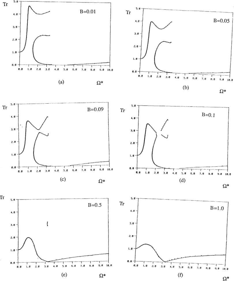
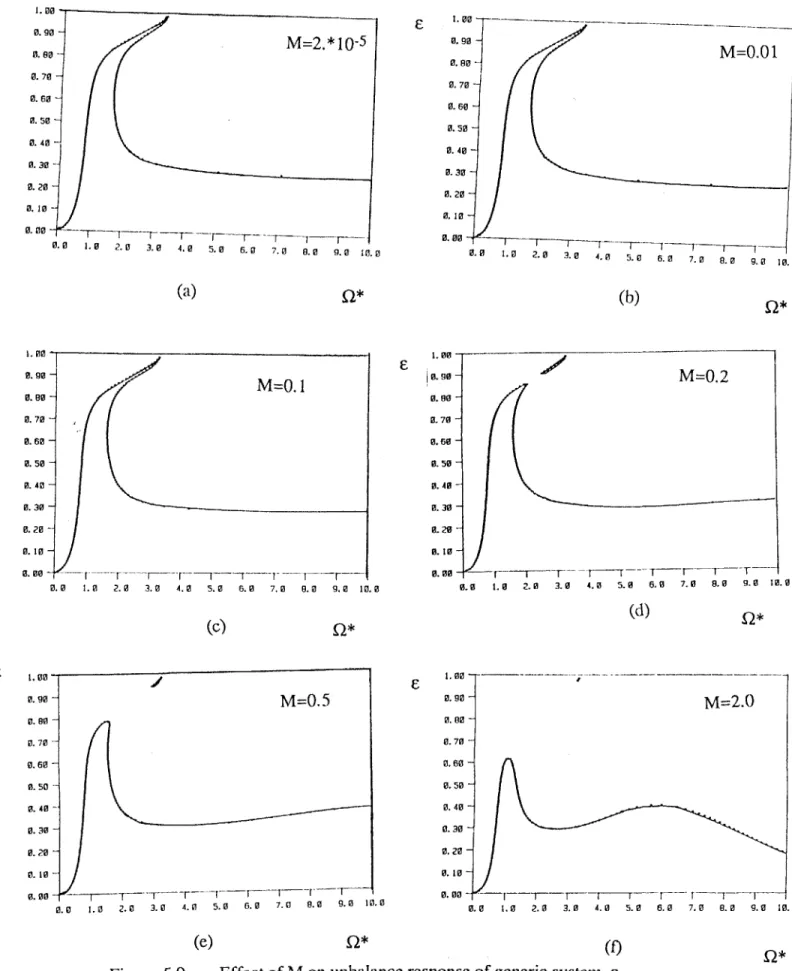
5.4 Parametric studies of unbalance response 99

5.4.1 Short squeeze film dampers 101

5.4.2 Long squeeze film dampers 115

5.5 Conclusions 132

Chapter 6 Conclusions 138

6.1 Review of thesis contents 138

6.2 Conclusions 140

6.3 Suggestions for future research 143

Bibliography 145

Chapter 1

Introduction

Squeeze film dampers (SFDs) are damping devices used essentially in aircraft gas turbine engines to damp the whirling vibrations of rotors. Their ability to attenuate the amplitude of engine vibrations and to decrease the magnitude of the force transmitted to the engine frame makes them an attractive rotor support.

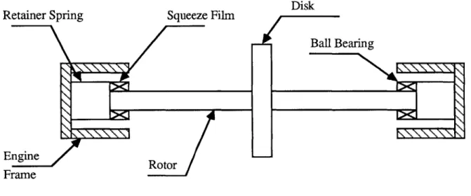
Figure 1.1 shows the construction of squeeze film dampers. The damper consists of an oil film in an annulus surrounding a rolling element bearing whose outer race is constrained from rotating, usually by a squirrel cage. Thus the spinning of the rotor does not reach the oil, and only when the rotor whirls does the oil film act to damp the motion. The squirrel cage serves to center the journal in the sleeve as well as to keep the outer race of the rolling element bearing from spinning.

1.1 Background

The earliest investigation of squeeze film dampers is probably that conducted by Cooper [15]t in the early sixties, in which he concluded that squeeze film dampers are adequate for damping the whirling vibration of rotating machinery. In his experiments he observed "bistable" operation of the rotor, that is the rotor would exhibit a jump from a certain whirling orbit to another at some frequency. This is the classical jump

Inner Race of Ball Bearing Oil FilmRor Housing Outer Race of Balls Ball Bearing Squeeze Film Ball Bearing Squirrel Cage Engine Frame

U

Figure 1.1 Construction of squeeze film dampers

C-phenomenon, and perhaps this was the first indication of the nonlinear behavior of squeeze film dampers. In the early seventies, White [101] studied theoretically and experimentally the dynamics of a rigid rotor on squeeze film dampers. He was able to calculate the forces acting in the damper based on Reynolds equation of fluid lubrication, and he calculated the so called bearing* coefficients. He predicted, both theoretically and experimentally, three steady state orbits of the rotor journal at the same frequency, but using a stability analysis he found that only two of them were stable. This confirmed Cooper's predictions for the jump phenomenon.

Since then squeeze film dampers have been widely used in aircraft gas turbine engines, and consequently the squeeze film damper (SFD) literature is quite rich. In the following we are going to highlight several of the investigations that are pertinent to this thesis, while a more complete list can be found in the bibliography. The quest of the previous investigations has been to faithfully describe the SFD theoretically, and to determine its effects on the dynamics of rotors that incorporate SFDs. These are the goals that this thesis tries to achieve. Other goals for previous investigations have been to experimentally test SFDs to determine the accuracy of the available theories and explore new configurations of SFDs.

Mohan and Hahn [57] studied the dynamics of a rigid rotor in squeeze film dampers. They obtained the steady state response by assuming a circular whirl, and they did parametric studies to determine the effect of the damper on the dynamics of the rotor, and the force transmitted to the engine frame, and also to determine the maximum rotor unbalance at which the damper is effective. They concluded that the squeeze film damper is generally an effective damping device, but for a badly designed damper, the transmitted

* _{In the literature the words 'damper' and 'bearing' have been used interchangeably to refer to squeeze film}

force can be magnified rather than attenuated, and this could lead to the failure of the engine.

Cunningham, et. al. [20], demonstrated the possibility of using design data for a SFD designed on the basis of single mass flexible rotor analysis, and applying it for the design of a SFD for a multi-mass flexible rotor. In an experimental parametric study, Tonnesen [97] was able to show that the forces in the damper agree with the n-bearing theory. Gunter, et. al. [29], numerically studied the nonlinear response of aircraft engines incorporating SFDs, and they were able to show that the rotor exhibits the jump phenomenon, and, under unidirectional loading, subharmonic whirl motion may exist. This was later verified experimentally by Sharma and Botman [77], who observed nonsynchronous whirl in their test rig, although they did not associate it with unidirectional loading.

Rabinowitz and Hahn [65] studied the steady state orbits for a flexible rotor incorporating SFDs. They did a parametric study to determine regions of unacceptable behavior of rotors due to SFDs. They also did a stability analysis of the steady state orbits they obtained [64]. Taylor and Kumar [85] did an investigation of the numerical integration techniques used to determine the response of a rigid rotor in SFDs. They were able to demonstrate the following drawbacks for numerical integration: a) only stable solutions could be found, b) false convergence, c) in regions of multiple-valued response, finding all possible solutions involves tedious trial and error, and d) the particular algorithm and convergence criteria used in the iterative approach determine the accuracy and credibility of the results. This motivated them [86] to find closed-form steady state solutions for a rigid rotor in squeeze film dampers by assuming a circular orbit. More recently, Guang and Zhong-Qing [27] used a similar technique to do a parametric study of a flexible rotor incorporating SFDs.

1.2 Fluid inertia

The above mentioned analyses are all based on Reynolds equation, which neglects the effects of fluid inertia. This has been a good assumption, since the dampers are usually operating at a very low Reynolds number. But as the speed of aircraft engines increases and as the trend of using lighter viscosity oils prevails, the values of Reynolds number for SFDs in practice have been continually increasing, and the need for a model that includes fluid inertia becomes a necessity.

Recently, in their experiments on squeeze film dampers Tecza, et. al. [87] showed that fluid inertia may be a significant factor in determining the dynamic characteristics of squeeze film dampers. This has prompted several investigations of the effects of fluid inertia in squeeze film dampers. Tichy [92] provided an explanation for the importance of fluid inertia in squeeze film dampers versus journal bearings. He later published experimental results to show the effect of fluid inertia [94].

Several identification techniques have evolved (especially in the United Kingdom) in the last few years, to experimentally determine the dynamic forces in SFDs, including fluid inertia. Amongst the workers in this field are Burrows et. al. [9] and Ramli et. al. [69]. For a comparison of the identification techniques used for estimating SFD coefficients see Ellis et. al. [22].

Perhaps one of the first attempts to study the effects of fluid inertia in hydrodynamic bearings, is the work of Smith [80] in the mid sixties. Using a unique form of Reynolds equation, he was able to obtain inertia force coefficients for journal bearings, and his conclusion was that the effect of fluid inertia in oil film bearings is to introduce an

added mass to the rotor and this may affect the dynamics of the rotor especially for short stiff rotors on wide bearings. Approximately a decade later Reinhardt and Lund [70] used a perturbation solution for small Reynolds number to obtain the force coefficients of journal bearings. They showed that fluid inertia introduces rather small corrections to the damping and stiffness coefficients of journal bearings and they also provided plots of inertia coefficients versus the eccentricity. They had to solve a set of differential equations numerically to arrive at these plots. Another notable paper, is the work of Szeri et. al. [84]. They used a technique based on averaging the inertia forces across the film, to obtain the force coefficients in a squeeze film damper. They also had to solve the resulting differential equations numerically. A recent paper by Ramli et. al. [68] compares the results of Smith, Reinhardt and Lund, and Szeri et. al.; and concludes that they are in good agreement, especially for short bearings. It is pointed out, however, that Smith's approach has the advantage of computational simplicity, and leads to fairly simple asymptotic analytical expressions for very short, and very long bearings.

In the literature, the methods used to handle inertia effects in hydrodynamic bearings can be divided into three categories. One method is to use a perturbation series in Reynolds number. Representative of this category are Tichy and Wiener [96], Jones and Wilson [42], and Reinhardt and Lund [70]. The solution thus obtained is valid for small values of Reynolds number. A second category is based on averaging the inertia forces across the film. Amongst those in this category are the work of Constantinescu [13], Szeri, et. al. [84], and San Andr6s and Vance [71,72]. The third category represented by Tichy and Modest [95,56] is based on a stream function approach to the linearized momentum equation, thus convective acceleration terms are neglected. All these techniques when applied to fluid film bearings result in quite a cumbersome solution, and the first two techniques require the solution of a set of differential equations numerically ([70] and [84]).

The results of all these researchers indicate that the classical lubrication theory is in error with respect to the pressure field and the inertia forces, which can dominate at higher Reynolds numbers. On the other hand, they all seem to indicate that the velocity field predicted by the classical lubrication theory is not greatly affected by fluid inertia for Reynolds number in the range of usual application of squeeze film dampers. In fact, the method of averaged inertia is based on the assumption that the velocity profiles predicted by the classical lubrication theory are not changed much by fluid inertia.

1.3 Thesis goals and outline

The literature articles surveyed in the previous pages seem to indicate that fluid inertia is an important factor in the dynamic characteristics of SFDs. It also seems that a model of fluid inertia forces in SFDs, including forces due to convective acceleration, has yet to be developed. This model should be simple enough to be easily used in rotordynamic analyses. Also the effects of fluid inertia on the dynamics of rotors incorporating SFDs, especially on the nonlinear behavior of the system, is yet to be investigated.

The goals of this thesis are to obtain a better model of squeeze film dampers, namely to include fluid inertia effects on the forces generated in SFDs, and to incorporate this simple model in a dynamic analysis of a Jeffcott rotor incorporating squeeze film dampers.

To achieve these goals, we start in chapter 2 by deriving the damping forces acting in a squeeze film damper. Reynolds equation for fluid lubrication is first derived and both the short and the long bearing approximations are used to obtain the pressure equation in SFDs. The pressure is then integrated to obtain the damping forces. The damping forces

are sensitive to the cavitation effects in the oil. If the oil film is cavitated we use the n-bearing theory, otherwise we use the full or 2n-n-bearing theory.

To include fluid inertia effects in the model, we find that the simplified Navier-Stokes equations for SFDs are nearly impossible to solve, so we resort to an approximate method. It is well known§ that if the kinetic coenergyt of the fluid could be calculated, then the fluid inertia forces can be determined from the kinetic coenergy, by using Lagrange's equations. But the kinetic coenergy is not known beforehand, so we assume that the velocity profiles can be approximated by those obtained from the inertialess solution based on Reynolds equation. As discussed in the previous section this approximation is used in the method of averaged inertia. The inertia forces are then calculated using Lagrange's equations of motion.

Before applying this approximate technique to obtain the inertia forces, to squeeze film dampers, we apply it to more elementary squeezing flows. This is both to verify that the approximate method based on calculating the kinetic coenergy is sufficiently accurate, and to understand better the mechanics of squeezing flows. Chapter 3 starts by describing two elementary cases of squeezing flows, namely the Poiseuille flow due to squeezing motion and the direct squeeze flow, as limits of the flow in a SFD. The Poiseuille flow is a linear problem and is solved completely including fluid inertia. It is shown that the velocity profiles do not change much due to fluid inertia for Reynolds number in the range of usual application of SFDs. This justifies the approximation of the kinetic coenergy based on the velocity profiles of the inertialess solution. The fluid inertia force in Poiseuille flow predicted by the approximate method, is shown to be the limit of the fluid inertia force as

§ See for instance Milne-Thomson [55].

Reynolds number goes to zero, and is also shown to be a good approximation for Reynolds number in the range of usual application of SFDs.

The squeeze flow is more complicated since it is nonlinear because of the presence of convective acceleration. Also the moving boundary results in time dependent boundary conditions. The problem is linearized and the inertia force due to temporal acceleration only is predicted and is shown to be in excellent agreement with that predicted by the approximate method based on the kinetic coenergy, hereinafter called the kinetic coenergy method, for Reynolds number in the range of usual application of SFDs. In this case Lagrange's equations have to be supplemented to include the effects of the fluid particles that leave the control volume carrying kinetic energy, as described in the appendix. Also the kinetic coenergy method predicts an additional term, which is shown to be due to convective acceleration, by an approximate solution of the nonlinear squeeze flow problem by the method of averaged inertia. The conclusion of this chapter is that the kinetic coenergy method adequately predicts the fluid inertia forces in squeezing flows for Reynolds number in the range of usual application of SFDs.

In Chapter 4 the kinetic coenergy method is applied to both the short and long squeeze film dampers. The dampers' inertia coefficients are derived and are shown to be nonlinear functions of the eccentricity of the journal in the bearing. These inertia coefficients represent the added mass to the journal. The fluid inertia forces are then obtained by using Lagrange's equations of motion. For the short squeeze film dampers, as in the squeeze flow case, Lagrange's equations have to be supplemented to include the effects of the fluid particles that leave the control volume carrying kinetic energy. Finally, the solution of the Navier-Stokes equations for the case of a small circular-centered whirl orbit is presented, and it is shown that the fluid inertia forces predicted by the kinetic

coenergy method is a good approximation to the forces in the damper for Reynolds number in the range of usual application of SFDs.

Chapter 5 discusses the dynamics of a Jeffcott rotor incorporating squeeze film dampers. The equations of motion are derived and it is shown that the steady state unbalance response can be obtained by assuming circular-centered whirling motions. Thus the resulting nonlinear algebraic equations are solved to obtain the unbalance response of the rotor. The simple solution for the steady state allows for parametric studies of the system to be made, and the effect of fluid inertia on the steady state dynamics of a rotor incorporating SFDs is explored.

Chapter 6 is the conclusion of the thesis. The problems attacked in this thesis are reviewed and the contributions and conclusions of the thesis are presented. Suggested topics for further research are also discussed.

Chapter 2

Damping Forces In Squeeze Film Dampers

In this chapter, we present the basic analytical tools required for the analysis of squeeze film dampers (SFDs). We first derive Reynolds equation for fluid lubrication from basic principles, then we derive the damping forces obtained by both the long and short bearing approximations of Reynolds equation. We also consider the effects of cavitation on the damping forces.

To include fluid inertia in the analysis, we find that the simplified Navier-Stokes equations for SFDs are nearly impossible to solve. To overcome this problem, we present an approximate method based on calculating the kinetic coenergy of the fluid, and using Lagrange's equations of motion to obtain the inertia forces in the damper. This method is outlined here, and will be discussed in detail in subsequent chapters.

2.1 Reynolds equation

Reynolds equation for fluid lubrication is an equation that the pressure in the damper has to satisfy. It is based on the solution of the continuity equation and the simplified Navier-Stokes equations subject to the boundary conditions in the damper.

In a squeeze film damper (SFD), the ratio of the clearance c to the radius R is very small, C/R = O(10-3), thus we can assume that the effects of curvature on the damper are

negligible and we can use a cartesian coordinate system in analyzing the flow in the damper. In addition, the following assumptions are going to be made [82]:

1- The variation of the pressure across the film is small and can be neglected. 2- The flow is predominantly two-dimensional ( circumferential and axial). 3- The flow is laminar, and incompressible.

4- The flow is fully developed and steady.

5- The rate of change of any one velocity component along the film is small compared to the rate of change of the same velocity component across the film.

6- Fluid inertia can be neglected.

y

t

0

r

'I X

x

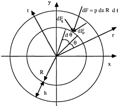
Figure 2.1 Squeeze film damper

Figure 2.1 shows a SFD, and the coordinate system used. The film thickness h at any given location is given by

h = c -e cos 0

where e is the eccentricity of the journal and 0 is measured from the positive r-axis of the whirling coordinate system (r, t, z). The z-axis is perpendicular to the plane of the paper.

1 00

Also shown in Figure 2.1, the stationary coordinate system (x, y, z) and the angle p which

is measured from the positive x-axis, and 0 = p - Nf. For a steady circular whirl N = ot,

where co is the whirling frequency of the journal and t is time.

Since we assumed that the effects of curvature can be neglected, we can use the stationary cartezian (X, Y, Z) coordinate system shown in Figure 2.1, (with the Z-axis perpendicular to the plane of the paper), to describe the flow. To an observer in this coordinate system, because c/R is small, it appears as if the damper is unwrapped, as shown in Figure 2.2. The upper surface in Figure 2.2 represents the journal, while the lower surface represents the bearing. The motion of the journal, i.e. the upper surface in Figure 2.2, results in the motion of the fluid in the clearance between the two surfaces. Due to the motion of the journal, the upper surface in Figure 2.2 travels in a wave-like fashion, and also changes its shape if the journal is moving radially. It should be noted that since the flow in the damper is cyclic, i.e. the conditions at p = 0 are the same as those at p

= 2n, then the model of Figure 2.2 is repeated every 2 n R in the X-direction.

Y

4 R y

x

Figure 2.2 Unwrapped squeeze film damper

Using the coordinate system and the assumptions described above, the Navier-Stokes equations reduce to

ap DIU(2.1)

= 0 (2.2)

(2.3)

where p is the pressure, u is the velocity of the fluid in the X-direction, w is the velocity of the fluid in the Z-direction and p is its viscosity .

Since p is independent of Y (equation (2.2)) thus we can integrate equations (2.1) and (2.3) with respect to Y using the boundary conditions

At Y=O u=0 w=O

At Y=h u=U w=O

Thus we get U 1 ap 2 h Y (2.4) 2 =t 2DX ( Y Y h ) + TU(24 W = (Y2 -Yh) (2.5) 2 g a For the continuity of flow

au iv aw _(2.6)

x+

T-+ -5z= 0(2)

where v is the velocity of the fluid in the Y-direction. Instead of integrating equation (2.6) over Y from 0 to h [62,82], to obtain Reynolds equation, (with the implication that the continuity of flow is satisfied on the average), we are going to determine v from equation (2.6). Thus

au a

v=- - dY - a dY+C

where C = C(X,Z) is yet to be determined. Substituting for u and w from (2.4) and (2.5), we get

1 Z) y3 y2 h ) ap ]+a y3 y2 h ) 2p a (y2 U

The above equation has to satisfy the following boundary conditions

At Y=O v=0

At Y=h v=V

The first boundary condition implies that C = 0, while the second gives us Reynolds equation for fluid lubrication

D( h' Dp ) + h' ap h (2.7)

3X p3X + BZ BZ = 12 V+ 6U -L+ 6h a (.7

If the journal has a radial velocity 6 in the r-direction of Figure 2.1 and a tangential velocity e* in the t-direction, then U and V, the velocities of the journal surface at any 0, become (see Figure 2.3)

U = e * cos 0 - e sin 0 (2.8) V = - e * sin 0- 6 cos 0 t _U V

e

Figure 2.3 Journal velocities

Since X = Rp and Z = z, then Reynolds equation for a squeeze film damper, in the (r, t) coordinate system, becomes

1 a h3 ap a hc3 ap _os0

R 7~p p R a~p Tz+

-

-

after neglecting terms of order c/R in the right hand side of equation (2.9).

Equation (2.9) is quite difficult to solve in closed form. Infinite series solutions for equation (2.9) exist [100], and it can be solved numerically [62]. Yet, for rotordynamic applications, it is beneficial to have a closed form solution for the forces acting on the journal, both to gain a better understanding of the dynamics of the rotors due to the oil film, and to reduce computation time for more involved rotordynamic analyses. Fortunately, two mathematical approximations to Reynolds equation exist that rely on the physical dimensions of the damper. These are the short and long bearing approximations to Reynolds equation and are presented in the following sections.

2.2 Short bearing approximation

For dampers with a length to diameter ratio up to 0.25, the short bearing approximation is a good approximation to Reynolds equations [62]. In the short bearing approximation, it is assumed that the damper is so short in the z-direction that the pressure gradient in the p-direction is much smaller than that in the z-direction, and thus the flow is essentially in the axial direction. The above statement is true even for sealed dampers, if the dampers are short. The dynamic pressures that are present in the damper are so large (of the order of a thousand psi) that no simple seal can stop the axial flow.

Using the short bearing approximation, Reynolds equation, equation (2.9) reduces to

z (z h' = -12 ( e * sin 0 + e cos 0)

Integrating twice with respect to z with the boundary conditions p = 0 at z = i IJ2

where L is the length of the damper, we get for the pressure

6 g L2 2) .. .

p =

T-

z

h

and the flow velocities u and w can be obtained by substituting from (2.10) into (2.4) and

(2.5) respectively. For future reference the w velocity profile is given by

6 z(YY 2~

W = z h 2 ( e * sin 0 + e cos 0) (2.11)

The damping forces can be obtained by integrating the pressure, equation (2.10). Thus the radial and tangential forces Frc and Ftc acting on the journal are given by (see Figure 2.4) L 0 - 02 Frc =

J .

Substituting for the pressure from equation (2.10) and integrating over z we get

p RL 3 02 cos20 . RL3r 02 cos e sin d

Frc = 3 -30 dO6- 3 f3 O e*

c

f1

(2.14)

pR 3 02 cosRL 3 02 sin2 0

_

jiR

J

1cos in

_(1-Ecos9)

F = c 3 _{0 ol1 - FCs0) O -}

_J

(2.15)

where e = e/c is the eccentricity ratio. The limits of integration 0₁ and 02 represent the

extent of the fluid film.

If there is no cavitation in the damper the limits of the integration are 01 = 0 and 02

= 2n. This would be the case if we had a highly pressurized damper. For a cavitated

phenomenon, and there is a lot of research going into cavitation in fluid film bearings [59,

99] and more involved analytical models for cavitation exist, but the t-bearing theory is the most acceptable theory in the literature of oil film bearings probably because of its simplicity. y t R h x

Figure 2.4 Forces on element in the damper

For a x-bearing, the oil film is assumed to extend in the region of positive pressure. Since the fluid cannot sustain tension, the region of negative pressure is assumed to be at zero pressure. The region of positive pressure is determined from equation (2.10), that is it extends from 01 such that

01 = tan~1

(-

?

I

Thus the oil film boundaries are moving such that the journal velocity vector acts in the direction of the center of the film. For a nearly circular whirl, the limits of integration can be taken to be 01 = 0 and 02= R for a counter-clockwise whirl. For a circular clockwise whirl the limits of integration can be taken to be 01 = x and 02= 2n. If the journal is travelling radially outwards then the limits of integration are 01 = - n/2, and 02= K/2.

Returning to the forces Frc and Ftc of equations (2.14) and (2.15), which may be written in the form

Frc = - Cr- C, e $ (2.18)

Frc = - C, i C, e $(2.19)

where the coefficients Crf, Ctt, Ctr and Crt are the damper's damping coefficients, and are given by R L3 02 cos2 c 3 1 ( 1 -C cos 0) 3 = R Lf 02 sin 0 c 3 f 1 ( 1 -e cos 0)3 C= R L 92 cos 0 sin 0 c 0 (l 1 -C coS 0)3 and Ct1 = C

It can be seen from equations (2.18) and (2.19) that the damping coefficients represent a symmetric tensor relating the force vector to the velocity vector. This means that the oil film is not isotropic, we get different damping forces when the journal moves in different directions. Also the cross-coupling damping coefficients Crt and Ctr imply that we get both radial and tangential damping forces even if the journal is moving in the tangential direction only, for instance.

For a t-bearing, with a journal executing a nearly circular counter-clockwise whirl, the coefficients Cfr, Ctt, Ctr and Crt take the form

pR L3 =* gRL3 _{* = R L 3} 3 Crr , Ctt 3 Ctt , Crt= 3 Crt c c c Crr = - (2.20)

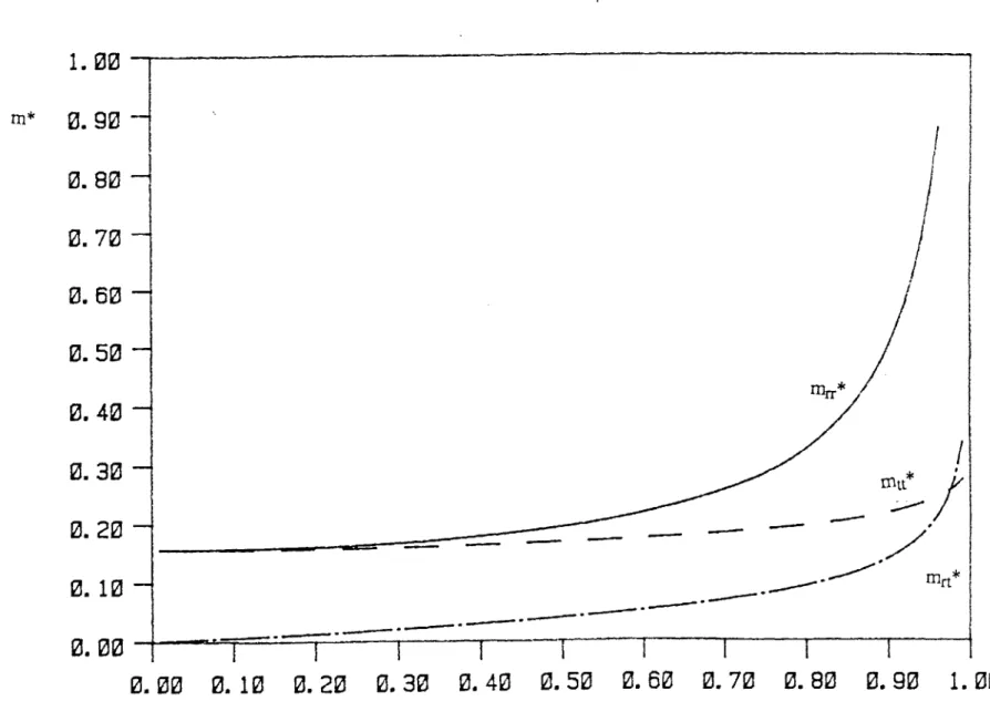
2

These coefficients are plotted in Figure 2.5, versus the eccentricity ratio, from which it can be seen that the damping coefficients increase drastically with the increase of the radius of the orbit, and become infinite as e approaches 1. Thus as the journal executes a larger orbit the fluid exerts a larger resisting force. For a 2n-bearing the coefficients Crr and Ctt are double those for a i-bearing and Crt and Ctr are zero.

2.3 Long bearing approximation

The long bearing approximation is based on the assumption that the damper is infinitely long in the z-direction such that the pressure gradient in the 6-direction is much larger than that in the z-direction, and thus the flow is essentially in the circumferential direction. The long bearing approximation is valid for dampers with L/D > 4, or for tightly sealed dampers.

For long bearings, Reynolds equation, equation (2.9) reduces to 1 h L... a _{-- 12 ( e * sin 0}

+ e cos 0)

I T twi wt R t w

I

/

/

10.

0

-9.0

-

8.0-

7.0-6. 0

5.

0

4. 0

-

3.0-

2.0-I

/

/

_Ctt*

-

I

1-

0. 00

0. 10

0. 20

0. 30

0. 40

0. 50

0. 60

0. 70

0. 80

0. 90

1. 00

Nondimensional damping coefficients for the short damper

Crt*

1.0-0.0

/

12 g R2

r

where C1 and C2 are constants of integration. With the aid of a table of integrals [4], the

above integrations can be performed, thus the pressure becomes

6 p R2 c ( 1 - cos )2 12 R2 sin e (1+2 62) sin 0 + e 2 2 c 3 2(1 - 2) (1 - E coS O ) 2 (1 - E2 2 (1 - -ccos ) 3 E- 1 -F + Cos 0 +2( _{1 - 2)5/2 cos} 1 -Eo2:I C esin 0 3 c sin e 2(1 -2) (1 C-cos )2 2(1 -2)2 (1 - E coS ) (2+E2) 8 _1 - E + cos 0 2( - 2) 12 kA-Ecose + C2 (2.23) where 8 is defined as S=1 1 sin 0 >! 0 -1 sin 0 0

The pressure has to satisfy the condition of periodicity, i.e. p(O = -R) = p(O = n). At 0 = 7

the film thickness is at its maximum and thus the lowest pressure occurs at this section. Since we are interested in the dynamic pressures only, we can assume without any loss of

generality that the pressure at 0 = 7 is equal to zero. Thus the boundary conditions that

equation (2.23) has to satisfy are

at 0 = -7 p = 0

Using these boundary conditions C₁ and C2 are evaluated to be 2 12g R . 32 S C 3( _{2 + 2 )} 6p2 and C2 =- g3 1 2 cF e (1+E)2 Finally the pressure is given by

6l R2 10

C 3 E F( l - ECOSO 92

1

E (1l + E )2 I

S2

]

2 + E-2) _{1 _- E COS )2(}

(2.24)

The flow velocities u and w can be obtained by substituting from (2.24) into (2.4) and

(2.5) respectively. For future reference the u velocity profile (neglecting terms of O(c/R))

is given by U = 6 R Y h 38

.1

The damping forces, as in the short bearing case, are obtained by substituting the pressure from equation (2.24) into equations (2.12) and (2.13).

tangential damping forces acting on the journal are

Frc 6 R3 L 0 2[ cos 2 C 3 fol E ( l - E coS 92 12 F = - 6gR3 L 3 c e.

Thus the radial and

cos 0

]

E(1+ E)2 I

gR L J sin 0 cos 0 ( 2 - E cos)

C 3 f01 (2+e 2 )(1-EcoS0) dO e Nf 2 _{sin 0 2 sin} O 101

[

c

sin2 0 (2- EcCos )HA

2 2 (2 2+ E2) (1l - E cos 0 ) and (2.26) (2.27) Y 2 h 2 3

Equations (2.26) and (2.27) can be written in the form of equations (2.18) and (2.19)

Frc = - C 6 Crt e (2.18)

FtC = - Ctr- Ctt e

Y

where Crr, Ctt, Crt and Ctr are the damping coefficients and are given by

6 3 L 02 cos e cos

1

It can be seen from equations (2.18) and (2.19) that the damping coefficients represent an unsymmetric tensor relating the force vector to the velocity vector. As for the short bearing, this means that the oil film is not isotropic.

Also here we are going to adopt the n-bearing theory for the cavitated damper and the 2it-bearing for the uncavitated damper. For a cavitated damper executing a nearly

circular whirl, the limits of integration are 01 = 0 and 02 = 7c. Thus the damping

coefficients become pR3LR R 3R3L*

c

c

* 24

Ctr = (2.31)

( 1+)( 1-E )

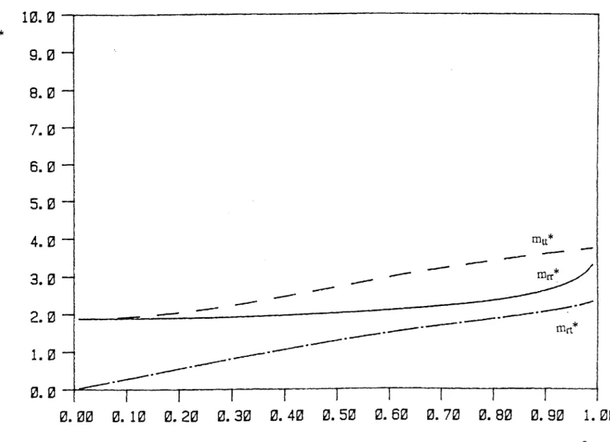
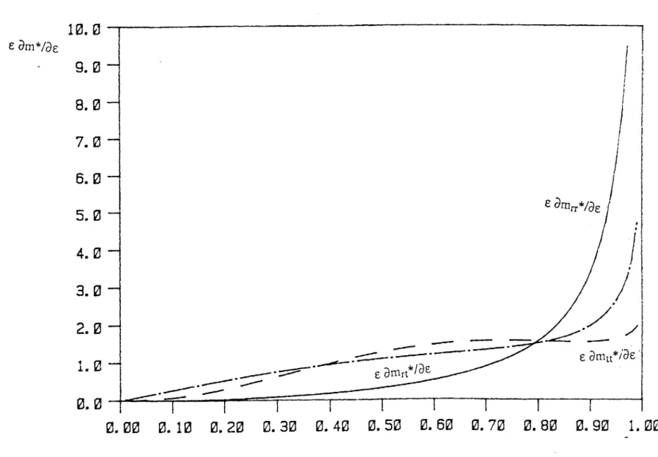
These coefficients are plotted in Figure 2.6, versus the eccentricity ratio, from which it can be seen that, as in the short bearing, the damping coefficients increase drastically with the increase of the radius of the orbit, and become infinite as E approaches 1. Thus as the journal executes a larger orbit the fluid exerts a larger resisting force. For a 2n-bearing the

coefficients Crr and Ctt are double those for a 7c-bearing and Crt and Ctr are zero.

Comparing the damping coefficients of the short damper with those of the long damper, we find that the damping coefficients of the long damper are relatively larger than those of the short damper, i.e.

Ciong =0 12RIn

Cshort

hort

Thus for example, if Riong = Lshort, then Clong=12 Cshort. This is to be expected since the oil in the short damper flows axially, and thus is squeezed out of the damper, while for the long damper the oil flows circumferentially and is forced to resist the motion. Also the damping coefficients of the short damper form a symmetric tensor, i.e. Crt = Ctr, while those for the long damper form an unsymmetric tensor.

2.4 Fluid inertia

Historically, as mentioned in the introduction, fluid inertia was neglected in the analysis of squeeze film dampers until it was demonstrated experimentally that fluid inertia does affect the performance of the dampers [87].

To include fluid inertia in the analysis and assuming an unsteady flow, but still retaining the rest of the assumptions, the Navier-Stokes equations become

50.

40.

20.

10.

0.-I

0.00

0.10

0.20

0.30

0.40

0.50

0.60

0.70

0.80

0.90

1.00

Nondimensional damping coefficients for the long damper Crr* Ctr* . -- -0

I

/*

Ctt*

I

I

I

I

I

I

au Du au au 1 ap a2U

+u - +v -+w +(2.32) 2--

- (2.33)

aw aw aw aw 1 ap a2w

+u T +v j + w -j- - + (2.34)

The above equations have to satisfy the following boundary conditions

At y=0 u=0 v=0 w=0

At y=h u=U v=V w=0

where U and V are given by equation (2.8). The above system of partial differential equations, together with the continuity equation, equation (2.6), is nearly impossible to

solve analytically except in very special cases.

To circumvent this handicap, we resort to an approximate method to calculate the fluid inertia forces in a squeeze film damper. Since the fluid in the damper moves only due to the motion of the journal, then if we were able to calculate the kinetic coenergy of the fluid, we can use Lagrange's equations of motion, with the velocities of the journal taken as the generalized velocities [55], to predict the inertia forces in the damper.

The kinetic coenergy of the fluid is defined as

T*= 1 p ( u2+v 2+ w2 ) dV (2.35)

where V is the volume of the fluid in the damper. Thus to calculate the kinetic coenergy we have to know the velocities of the fluid. But since we do not know the velocities of the fluid beforehand, we are going to assume that the velocity profiles predicted by the classical lubrication theory are a good approximation of the actual velocity profiles, even at relatively high squeeze Reynolds numbers. This approximation has been used before in conjunction with the method of averaged inertia [13], and is justified by the results of previous

researcherst that indicate that the velocity field predicted by the classical lubrication theory is not greatly affected by fluid inertia for Reynolds number in the range of usual application of squeeze film dampers.

In the next chapter, it is going to be shown that this assumption is reasonable in simple squeezing flows for Reynolds numbers in the range of usual application of squeeze film dampers. The application of this technique, hereinafter called the kinetic coenergy method, to obtain fluid inertia forces in squeeze film dampers is illustrated in chapter 4.

Chapter 3

Fluid Inertia Effects In Squeezing Flows

As mentioned in the introduction, the results of previous researchers indicate that the classical lubrication theory is in error with respect to the pressure field and the inertia forces, which can dominate at higher Reynolds numbers. On the other hand, they all seem to indicate that the velocity field predicted by the classical lubrication theory is not greatly affected by fluid inertia for Reynolds number in the range of usual application of squeeze film dampers.

The aim of this chapter is to study the basic constituents of the flow in a squeeze film damper, namely, the Poiseuille flow produced because of squeezing motion, and the direct Squeeze flow, both to understand the mechanics of squeezing flows and to illustrate the effectiveness of the kinetic coenergy method introduced in the previous chapter. It will be shown that this approximate method agrees favorably with the full solution, including convective acceleration.

3.1 Poiseuille flow resulting from squeezing motion

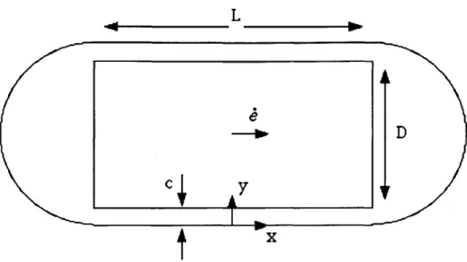
Consider a block of a rigid material having length L, width D and thickness b moving with a velocity e in a chamber filled with an incompressible fluid, as shown in Figure 3.1. This can be considered as a simplified squeeze film damper (SFD). Figure 3.2 shows a SFD moving radially outwards with a velocity 6. Comparing Figures 3.1 and 3.2,

LD

Figure 3.1 Schematic of a block moving in a fluid-filled chamber.

we can see that the block in Figure 3.1 represents the journal in Figure 3.2, but is simpler in the sense that the flow past the block in the clearances moves in a straight channel, while the flow past the journal in the damper clearance moves in a curved channel. We assume that, in the Poiseuille flow of Figure 3.1, the side chambers are large, such that the pressure is uniform in these side chambers.

Poiseuille flow

Squeeze flow

Let c be the clearance between the block and the chamber, with D/c >> 1, and consider a stationary reference frame (x,y) attached to the chamber with the x-axis coinciding with the lower surface of the chamber. Since the problem is symmetric the flow in the upper and lower clearances is the same, and only the flow in the lower clearance will be obtained. The classical lubrication theory solution (inertialess solution) will be presented first, followed by the solution of the problem including the inertia of the fluid.

In the classical lubrication theory, i.e. neglecting fluid inertia, the x-momentum equation reduces to

d2u _dp ₀

d=0 (3.1)

dy2 dx

where t is the viscosity of the fluid, u is the velocity of the fluid in the x-direction and dp/dx is the pressure gradient. The y-momentum equation is

dp = 0 _(3.2)

dy

thus the pressure gradient dp/dx is independent of y. Equation (3.1) can be integrated twice with respect to y, with the boundary conditions

at y=0 u=0 (3.3)

at y=c u=e

thus the velocity u is given by

2

(

u = - d dp y _ c y (3.4)

To determine the pressure gradient recourse has to be made to the continuity of the flow in the chamber. The fluid squeezed by the block has to flow through the clearances. Therefore

C

Note that the negative sign in the left hand side of equation (3.5) is because the fluid and the block are moving in opposite directions. Substituting (3.4) into (3.5), the pressure gradient becomes (neglecting terms of order c/D)

dp pD .

d-= 6 -- e (3.6)

dx c3

and the velocity u becomes

u=-e-- -- l (3.7)

c c c c2

Also, the force F resisting the motion is F = - (pI-p2) D b

where pi and P2 are the pressures in front of the block and behind it, respectively. The negative sign is because the force F opposes the motion. By using (3.6), the force F becomes

p D 2 b L

F = -6 3 b (3.8)

c

The force F in equation (3.8) is proportional to the velocity of the block and is due to viscous effects.

The above analysis was for the case when fluid inertia is neglected. If the effect of fluid inertia is introduced equation (3.1) becomes

au 1 ap

a2u

-=- -+x - (3.9)

jat p Dx vay2

where p is the fluid density, v is its kinematic viscosity, and t is time. To solve equation (3.9) , for an oscillating block, assume u, p and 6 to have an eiOt time behavior. Thus, let

u = U eiot, p = P eiOt, and i = UO eiot, and equation (3.9) becomes

1 dP d2U

i OU=---+V 2 (3.10)

pdx _dy2

The pressure gradient is still independent of y, and we can solve the differential equation (3.10) for U, using the boundary conditions (3.3)

U i dP sinh (sy) - sinh (s(y - c)) - sinh (sc) sinh (sy) U (3.11) o p dx sinh (sc) sinh (sc) where s= 1( 1+i ) (3.12) and Re = o(3.13) V

is the Reynolds number. It can be shown that as Re -+ 0, equation (3.11) reduces to equation (3.4). Substituting equation (3.11) into equation (3.5), the pressure gradient becomes

i

Uo

i

dP _ L (3.14)

dx [2 - 2 cosh (sc)+ sc sinh (sc)] and the force F is

dP

F=-LDb--dx

and thus the nondimensional force

=F c

F* = 2

(3.15)

becomes

1

i Re[ s sinh (sc)+ - cosh (sc) -

-F* = - 2 siD (3.16)

[2 - 2 cosh (sc) + sc sinh (sc) ]

It can be shown that as Re -* 0, F* has the form (neglecting terms of O(c/D))

lim F*=-6[1+i 0.lRe] (3.17)

Re--O

which shows that as Re -+ 0, F* has a real part equal to that of equation (3.8) predicted by the classical lubrication theory. The real part of F* represents the viscous force, while the imaginary part represents the force due to the inertia of the fluid. Equation (3.17) shows that the inertia force, as Re -+ 0, is linear with Re, which is also nondimensional frequency. Figure 3.3 shows the nondimensional force F* plotted versus Re, using equation (3.16), for D/c = 1000. On the same figure the classical lubrication solution,

0.

-10.

-20.

-30.

1~

K

-40.

-50.

-. 50.I

20.

30.

40.

50.

60.

70.

80.

0

1I

90.

100.

Figure 3.3 Nondimensional forces acting on block in Poiseuille flow A

equation (3.8), is plotted for a sinusoidal velocity. It can be seen that the real part of the full solution deviates by only a few percent from the inertialess solution equation (3.8), for Re up to 50, which is the range of Reynolds numbers found in practice for squeeze film dampers [84]. The deviation increases to up to 50 per cent at Re = 100, but at that point the flow is totally dominated by inertia rather than viscous effects. In fact, the viscous force is equal to the inertia force at Re = 10, and for higher Reynolds numbers the inertia force is larger. The imaginary part of the force in equation (3.16), which represents the inertia force, is shown in Figure 3.3 to be nearly linear with Re. Also shown is the solution predicted by the approximate method, discussed in the next section, for the inertia forces.

It should be noted that the total force F, acting on the block is the real part of F* eiot, that is, from equation (3.17), the force acting on the block as Re -+ 0, is given by

F= - _{Lb 2 [ cos wt - 0.1 Re sin cot] (3.18)}

c

As an example of the effect of fluid inertia, it can be seen from equation (3.17) that the amplitude of the inertia force (for small Re) is given by

ULbD2 p 2

Fj

I

c

Thus the mass added to the block is

m = 0.6 p L b D (3.19)

c

while the mass of the block is M= PbLbD

where Pb is the density of the block. Thus the ratio of the mass added to the block due to fluid inertia to the mass of the block is

mDp

M 0.6Dp

If the block is made of steel, its density would be about Pb = 7800 kg/m3 and typically the density of oil would be about p = 800 kg/M3, and for squeeze film damper applications D/c is in the order of 1000, then m/M would be of the order of 60. This means that due to the huge velocities and accelerations in the clearances the mass of the block, which is made of steel, can be neglected with respect to the added mass due to the inertia of the oil. Also it can be seen from the above relationship that m/M increases as the clearance c decreases, this is because for smaller clearances the velocity and acceleration of the fluid in the clearance increases, and thus the added mass increases, even though the actual mass of the fluid film has decreased.

3.2 Kinetic coenergy method applied toPoiseuille flow

The flow velocity U in the full inertial solution can be obtained by substituting equation (3.14) into (3.11). The velocity profile thus obtained is plotted in Fig. 3.4 for D/c = 1000, and Re = 1, 10, 30, and 100. Plotted also is the inertialess velocity profile, equation (3.7), and it can be seen that they match nearly identically for low Re. This was expected, as discussed in the introduction, from the previous literature.

The approximate method is based on the assumption that the velocity profile is not changed much by the inertia of the fluid. Thus the flow can be assumed to be that of the classical lubrication theory, and the kinetic coenergy of the fluid can be calculated. The inertia forces acting on the block can thus be obtained by the use of Lagrange's equations.

Assuming that the fluid velocity is given by the inertialess solution equation (3.7), the kinetic coenergy stored in the fluid is then

Re= 1.0 Re=10.0 1.00 0.90 0.80 0.70 0.60 8.50 8.40 0.30 0.20 0.1 -0-00 -1000. -900. -000. -700. -600. -500. --400. -300. -200. -100. g. 1.00 0.90 Y/c 0.70 0.60 0.50 -0. 40 0.30 -0.20 5 - -3 - -18--000. -900. -- 000. -700. -600. -500. -400. --300. --200. --100. 0. U/UO U/U0 Re=100.0 Y/c 1. 00 8.98-0.80 0.70-0.60 -0.50 0. 40 0.30 0.20 8.18 0. 00 1 II -1000. -900. -00. -700. -600. -500. -400. -300. -200. -100. 0. Y/c 1.00-8.90 0.80-0.760 -0.60

(

Figure 3.4 Velocity profiles for Poiseuille flow for D/c=1000 Y/c

where dm is the mass of an infinitesimal volume of fluid flowing in the clearance. Therefore

T*= 2 p L b u2 _dy

Substituting for u from equation (3.7), we get (neglecting terms of order c/D)

T*= 1[0.6 pLbD2 ] 2 (3.20)

21 c

The added mass to the block is represented by the quantity between brackets in equation (3.20), which is exactly equal to the added mass predicted by equation (3.19). Equation (3.20) represents the kinetic coenergy stored in the fluid, but it is only a function of the velocity of the block d. The added mass to the block due to fluid inertia, means that we are representing the fluid particles with a point mass at the center of the block. Thus we can obtain the forces acting on the block due to fluid inertia by calculating the inertia force due to the point mass. If we take the velocity of the block 6 as our generalized velocity, then the generalized momentum in the direction of 6 is given by

S= 0.6 LbD2

ad c

Note that this generalized momentum acts in the opposite direction of the fluid velocity. Using Lagrange's equation of motion, the force due to the inertia of the fluid is

d (T* DT* pLbD2

F-=-- - - +-=-0.6 e

dt + ; e c

For i = UO cos wt, then e= - o UO sin ct and

Fj = 0.6 _c o UO sin ot (3.21)

which is exactly the same as that predicted by equation (3.18), for the full solution as Re -4 0. Equation (3.21) (in complex form) is plotted on Fig. 3.3 which shows the close agreement, especially at low Re, between the exact solution equation (3.16) and the approximate solution equation (3.21). The approximate solution has the advantage of simplicity, since it only requires the knowledge of the velocity profile predicted by the classical lubrication theory, without having to solve the partial differential equations of

motion including the inertia terms. It should be noted that we did not have to consider the kinetic energy of the fluid particles that leave and enter the system, since the fluid particles that enter the system at one side have the same velocity distribution as the fluid particles that leave the system from the other side. Thus there is no net gain or loss of kinetic energy. We will have to consider the flux of the kinetic energy from the system when we obtain the inertia force in the squeeze flow case.

3.3 Squeeze flow

The second constituent of the flow in a squeeze film damper is the direct Squeeze flow. Consider a flat surface moving downwards towards a stationary flat surface, and squeezing an L V h Y 1 x

Figure 3.5 Squeeze flow between two flat surfaces

incompressible fluid, as shown in Figure 3.5. Let the distance between the two surfaces be h and the length and width of the surfaces be L and b, respectively, and let h/L<<1. Consider an (x,y) frame attached to the lower surface at its center. Let u and v be the velocities of the fluid in the x-and y-directions, respectively, and p be the pressure. This can also be considered as a simplified squeeze film damper, by comparing Figures 3.5 and 3.2. At the point of minimum thickness of the oil film in Figure 3.2, the oil flow divides, and the oil flows in two opposing directions. This is very similar to the squeeze flow of

Figure 3.5. As the plate moves downwards, it squeezes the oil, which divides and flows in two opposing directions. Thus, the squeeze flow can be considered as a simplified model of the squeeze film damper. This becomes clearer if we compare Figures 3.5 and 2.2. The upper flat surface of Figure 3.5 approximates the upper curved surface of the unwrapped SFD of Figure 2.2, but it simplifies the analysis because the flat surface simplifies the boundary conditions and also because it moves vertically only, while the upper curved surface of Figure 2.2 moves both vertically and horizontally.

Here also the inertialess solution is presented first, followed by the full inertial solution. In classical lubrication theory fluid inertia is neglected. The momentum equation in the x- direction becomes

du _dp_

2 = 0 (3.22)

dy

where g is the viscosity of the fluid. The momentum equation in the y-direction reduces to dp _

dy

Thus, the pressure is independent of y, and also the pressure gradient dp/dx is independent of y. Integrating equation (3.22) twice with respect to y, with the boundary conditions

u=0 at y=0

(3.23)

u=0 at y=h

we get for the velocity u

2 2

U _{2 g dxw} h dp y _h y _{h 2} (3.24)

Notice that h is varying with time.

The continuity equation for a two dimensional flow is

+ = 0 (3.25)

)x

_ay

v=- - dy +C ax

where C=C(x) is yet to be determined. Substituting for u from (3.24) we get

h2 d2(2 3

V = + C _(3.26)

2 pt dx2 _(2h

3h 2 ₎

The boundary conditions that (3.26) have to satisfy are at y = 0 v = 0

(3.27) and at y = h v = dh/dt=li

The first boundary condition implies that C = 0, while the second gives us the following equation that the pressure has to satisfy

2

d p= 12

dx2 h3

Integrating twice with respect to x, with the boundary conditions at x = ± L/2, p = 0

assuming atmospheric pressure on the sides, the pressure becomes

L.

P=-6 [ T-x h (3.28)

and the force F is

L

F = bJ pdx = h3bL (3.29)

2h

and from equation (3.24) the velocity u becomes

6=-6 -- (3.30)

Notice that the velocity profile u for Squeeze flow is parabolic as that of the Poiseuille flow due to squeeze motion, equation (3.7).

To include the fluid inertia effects, the momentum equation in the x-direction becomes

Du iu au 1 ap 32u

-+u-+v-=--- +