Dynamics characterization for designing functional soft materials

(1)

Dynamics Characterization for Designing Functional

Soft Materials

by

William Robin Lindemann

Submitted to the Department of Materials Science and Engineering

in partial fulfillment of the requirements for the degree of

Doctor of Philosophy in Materials Science and Engineering

at the

MASSACHUSETTS INSTITUTE OF TECHNOLOGY

May 2020

c

○ Massachusetts Institute of Technology 2020. All rights reserved.

Author . . . .

Department of Materials Science and Engineering

May 8, 2020

Certified by. . . .

Julia H. Ortony

Associate Professor of Materials Science and Engineering

Thesis Supervisor

Accepted by . . . .

Frances M. Ross

Professor of Materials Science and Engineering

Chair, Department Committee on Graduate Theses

(2)

(3)

Dynamics Characterization for Designing Functional Soft

Materials

by

William Robin Lindemann

Submitted to the Department of Materials Science and Engineering on May 8, 2020, in partial fulfillment of the

requirements for the degree of

Doctor of Philosophy in Materials Science and Engineering

Abstract

In solutions, the dynamic behavior of soft materials is often critical to their func-tion. In biological materials such as proteins and peptides, the edict that ‘structure dictates function’ has been supplanted in recent decades by recognition that features like intrinsic disorder, conformational distribution, and solvent dynamics often play a part which is equally fundamental to the binding and reactivity of these materials. The same revelation holds for many other functional soft materials, including abiotic peptides and self-assembling materials, where function is controlled by the dynamic behavior of both the compound and the substrate. In this work, I elucidate the role of dynamics in several significant functional polyamides by the synthesis and charac-terization of samples spin-labeled for electron paramagnetic resonance (EPR) spec-troscopy. By this approach, I developed insight into several soft-materials systems, including abiotic peptide tags, combinatorially selected for bioconjugation; fibronectin mimetic peptides, designed for therapeutic purposes, biomaterials and drug delivery; and finally, novel, self-assembling polyamide materials designed for water purification and energy conservation.

Thesis Supervisor: Julia H. Ortony

(4)

(5)

Acknowledgments

When I was in high school, attending MIT was a dream that I never thought I would realize. For my first several months here, I still had trouble believing it. The experience has been challenging – in ways I expected, and in ways I never forsaw. I am inexpressibly grateful to the friends and family who bore me through it. This work is dedicated to you.

To my parents, Bill and Ruth: I can only say that I am incredibly grateful. For as long as I can remember, you have done nothing but support me. When I was excited by a new experiment or result, I knew I could make my best days better by calling you. And on my worst days, when life reduced me to a trembling ball of nerves, I knew that talking to you would make me feel better. Every time I’ve jumped off a cliff, you’ve both been there – cheering for me when I fly, but ready to catch me when I fall. I don’t know if I’ll ever be able to explain how much that has meant to me. Thank you, and I love you.

To my fiance, Molly Parsons: our relationship started 5 years ago, with a leap of faith. I don’t think either of us knew what we were in for when we started grad school, but through everything, I’ve been profoundly proud to have you on my team, and I’m glad, in turn, that you’ve chosen me for yours. You are my best friend, and I couldn’t have gotten here without you.

To my brother, Geordie: thank you so much, for being the only person in my family who knows what I’m talking about half the time. I’m so glad to have your voice in my life, and I appreciate the many times you’ve let me vent about grad school.

To my labmates and collaborators, new and old: thank you all for your advice, your understanding, your kindness, and your friendship. And thank you for tolerating my incessant yammering. I can’t imagine what this work would look like if I hadn’t had such a supportive and brilliant team of people standing in my corner.

And finally, to my advisor, Julia: you are truly the person who most completely shaped my graduate experience at MIT, and in myriad ways, you made this work

(6)

possible.

(7)

List of Figures

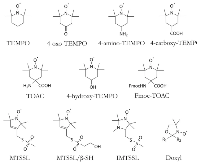
2.1 Common nitroxide probes used to study soft materials . . . 24 2.2 Energy levels in nitroxide radicals . . . 26 2.3 Peptide flow synthesis schematic . . . 34 3.1 MP01-Gen4 peptide reacts rapidly with a perfluoroarene capture agent

(CA) via nucleophilic aromatic substitution (S𝑁Ar) . . . 39

3.2 Experimental approach to dynamics measurements . . . 40 3.3 LC-MS elution profiles of MP01-Gen4 variants before S𝑁Ar reaction

and after EPR analysis . . . 47 3.4 LC-MS elution profiles of the MP01-Gen4 variants following S𝑁Ar

re-action and EPR analysis . . . 48 3.5 Estimated conversion yield of the S𝑁Ar reaction . . . 50

3.6 Arrhenius plots of residue-specific dynamics of MP01-Gen4 before and after reaction with MP01-Gen4 . . . 51 3.7 The initially disordered region of MP01-Gen4 experiences a greater

change in dynamics upon reaction . . . 53 3.8 S𝑁Ar Reaction is accompanied by a significant drop in diffusional

ac-tivation energy . . . 54 4.1 Predicted disorder probability for each amino-acid residue in the 1FNF

sequence, centered on the RGD site . . . 62 4.2 The structure of RGD-containing fibronectin fragments. . . 68 4.3 CW-EPR data superimposed over spectral best-fits for each FMP sample 69

(12)

4.4 Dynamic behavior at the RGD site changes discontinuously with length 70 4.5 Molecular dynamics simulations illustrate intra-chain hydrogen bond

formation in FMP peptides and fibronectin protein . . . 72 4.6 Ramachandran plots of the RGD site in 200 ns peptide simulations . 73 4.7 Distributions determined by pulsed dipolar spectroscopy and MD

sim-ulations describe the distances between the glycine of RGD and the N-terminus of each FMP peptide. . . 74 4.8 Displacement of fluorescently labeled fibronectin, bound to cellular

𝛼V𝛽3, by FMP peptides . . . 76 5.1 Self-assembly of planar nanofibers with spin labels tethered at known

distances off the surface . . . 82 5.2 The structure of (6), the AA tail coupled to polyproline to synthesize

compounds (2-5) . . . 83 5.3 Elution profiles (left), and mass-spectrometry (m/z) profiles (middle,

right) of HPLC-purified AA spin probes . . . 90 5.4 Arrhenius plots describe 𝐷𝑅 derived from EPR fits . . . 91

5.5 Representations of the 𝜒2

𝜈 landscape for a spectral fit . . . 93

5.6 Activation energies of diffusion, 𝑄, of spin labels tethered at known distances off a nanofiber surface . . . 95

(13)

List of Tables

3.1 Names and sequences of the MP01-Gen4 variants employed in this study 41 3.2 Crude yields and LC-MS data for MP01-Gen4 variants . . . 43 4.1 Fibronectin-mimetic peptide (FMP) designations, sequences, and exact

masses . . . 70 5.1 Spin-labeled oligoprolines tethered to the surface of AA nanofibers . . 89

(14)

(15)

Chapter 1 Introduction

1.1 Dynamic Behavior in Materials

For over 40 years, bioactive materials have played a pivotal role in the modern medicine. Bioactive materials, here defined as materials which interact constructively with cells in the human body, frequently hinge upon the incorporation of bioactive sites which provide functional value.

Few problems prove more vexing than studying and manipulating the conforma-tional behavior of these bioactive sites. While the community now accepts the impor-tance of dynamics to the activity of peptides and proteins1–3_{, the dynamic properties}

of these materials remain particularly difficult to characterize. Nevertheless, a few experimental techniques, such as nuclear magnetic resonance (NMR), quasi-elastic neutron scattering (QENS), and electron paramagnetic resonance (EPR), can pro-vide quantitative insight into the conformational dynamics of materials.

Dynamic behavior perhaps matters most to protein interactions. Proteins show tremendous potential as a tool for treating disease, healing injuries, and designing biocompatible implants and devices. By incorporating functional proteins or peptides into biomaterials, researchers have successfully facilitated bone repair4–7_{, the growth}

of nerve and brain cells8–11_{, the regeneration of dental pulp}12–14_{, and the formation}

of vasculature to speed the healing of wounds.15–17 _{Their high specificity of function}

(16)

finding the right protein for the job.

Although scientists recognized the importance of proteins in physiology over a century ago, we did not understand their chemical nature until the early 1950s.18

First, in 1949, Sanger succeeded in sequencing the terminal amino acids of insulin – demonstrating the high predictability of amino acid positions in these materials.19,20

The second great insight into protein properties came from Linus Pauling, who in 1951 predicted the helical structure of some proteins based on hydrogen bonding.21

The revelation that a protein’s structure and sequence help dictate its function gave birth to the field of molecular biology, paving the way for tremendous advances in science and medicine.

Over the next 60 years, we became more sophisticated in our attempts to charac-terize the structure and sequence of proteins. Today we have the protein data bank (PDB), which contains millions of crystallographic structures with atomic resolution, accessible to all, and typically confirmed using atomistic simulation and characteri-zation techniques such as NMR and X-ray scattering.22–31 _{Even in lieu of structural}

information, most proteins may be sequenced using mass spectrometry and database matching.32–34

In the 1960s, scientists began studying protein sequences in order to identify the regions involved in binding. We refer to these regions as ’epitopes’. The term, which originates in the field of immunology, initially applied only to subsequences of antigens (molecules that activate antibodies or T-cells).35 _{In contemporary usage within the}

biomaterials community, ’epitope’ refers to the active part of any protein. Epitopes have long interested immunologists, who aim to identify the active sites of antigens (sometimes called ’antigenic determinants’) in order to produce vaccines, viral in-hibitors, and other therapeutic agents.36–40 _{Scientists then began identifying epitopes}

of other proteins for use in bioactive materials. By producing synthetic versions of these epitopes, known as biomimetic or epitope-mimetic peptides, researchers aim to imitate the function of the parent protein, while avoiding the drawbacks (such as toxicity or difficulty of production) associated with its use.

(17)

identified five epitopes of myoglobin and attempted to form general conclusions about functional sites in proteins.41 _{In particular, Atassi advocated for the idea that all}

bonding subsequences of proteins: i) do not exceed six or seven amino acids, arranged consecutively; and ii) are very sensitive to mutation, losing most of their functionality with the replacement of even a single residue.

Although the scientific community still accepts some of Atassi’s conclusions, sci-entists have reported counterexamples or exceptions to many of them. For instance, some myoglobin binding sites use several, disjointed regions of the protein sequence, rather than one continuous subsequence.42 _{This led to the general classification of}

epitopes as continuous (sequential) or discontinuous (non-sequential). According to the work of Barlow, Edwards, and Thornton, discontinuous epitopes appear most often in globular proteins, since lengthy, continuous subsequences rarely reside at the protein surface.43_{Huang and Honda compiled a database of well-established examples}

of discontinuous antigen epitopes in 2006.44

One of the key ideas of twentieth century biology was the realization that in pro-teins, ’structure dictates function’. This model, called the lock-and-key mechanism for protein binding, remains fundamental to our understanding of the interactions be-tween proteins and other molecules. It states that protein interactions occur primarily as a result of protein structure. This is particularly true in the case of proteins that target small molecules. However, in the context of protein-protein interactions, this model has proven insufficient, failing to explain the natural ubiquity of intrinsically disordered proteins in nature. For instance, hub proteins, which interact separately with large numbers of other proteins, seem to accomplish this feat through confor-mational changes in the chain backbone.2 _{Most of these proteins display biological}

activity, despite the fact that they routinely diffuse through distinct structures over time.

These kinds of conformational variations occur regularly in nature, where proteins typically occupy a statistical distribution of distinct conformations, rather than one single conformation. A pair of mechanisms, known as the conformational selection model and the induced fit model, help to explain the role of conformation in protein

(18)

interactions.45,46 _{The conformational selection model assumes that structure remains}

fundamental to the role of protein binding, and that proteins can only bind at times when they have already folded into a conformation resembling their bound state. In contrast, the induced fit mechanism assumes that the presence of a binding target induces a conformational change in the protein structure. Both of these mechanisms occur in protein binding systems, although conformational selection appears more often than induced fit.45–49 _{In both of these models, binding kinetics depend upon}

the protein’s conformational distribution. This, in turn, provides the first indication of the importance of dynamics to protein binding.

In biotechnology, we typically desire sequences with high affinity and rapid kinet-ics. When proteins change conformation slowly, the rate of diffusion between distinct conformations limits the protein binding kinetics, and may even modify the binding equilibrium. Importantly, this does not mean that faster-moving sequences are neces-sarily better. For one thing, structure still remains the dominant factor in reactivity. A slow-moving structure with a highly stable binding epitope will bind much more effectively than a structurally unstable molecule experiencing rapid conformational change. Moreover, binding in peptides likely depends on their dwell-time in favorable binding conformations. However, these models certainly demonstrate that under-standing protein binding often requires a dynamic picture of these molecules, and an understanding of how complex properties like flexibility and the rate of conformational change affect functionality. Several studies support the importance of dynamics in protein binding.1–3,50,51 _{However, very few of these examine the relationship between}

sequence, structure, and chain dynamics. Generally, these factors interconnect. For instance, a computational study demonstrated that functionally distinct proteins with similar structures possess similar dynamic properties.52 _{Another study, analyzing the}

effect of mutation on chain dynamics, concluded that even after residue substitution, chain conformations and dynamics remain very similar to the unmutated protein.53

Experimental studies relating protein chain dynamics with function present a tremendous technical obstacle. Some techniques, such as NMR or QENS, enable direct observation of protein dynamics. Unfortunately, these techniques often require

(19)

isotopic labeling, a very difficult process in proteins and peptides.1,51,54 _Moreover,

these techniques require very high protein concentrations, making them unrepresen-tative of real, biological conditions. Most other tools for measuring protein dynam-ics (e.g. dynamic light scattering, DLS, and X-ray photon correlation spectroscopy, XPCS) measure the diffusion of the overall molecule, rather than local chain dynam-ics.

One of the simplest approaches for measuring site-specific dynamics is by us-ing electron paramagnetic resonance (EPR) – a technique that detects the motion of unpaired electrons in a material. Through the selective introduction of stable free-radicals as spin-labels, EPR allows site-specific measurement of chain motion in solution. Fitting the data with spectral simulations allows direct measurement of an unpaired electron’s rotational diffusion coefficient – a quantity that relates to the rate at which a protein backbone changes conformation. This allows highly quantita-tive calculations of backbone dynamics, which agree with observables computed via molecular dynamics simulations.55

The high sensitivity and site-specificity inherent in EPR measurements makes this technique substantially more robust than NMR and QENS measurements, because it is still useful for dilute or multicomponent systems. Nonetheless, it has its own challenges, including the difficulty of synthesizing and characterizing sample, and the challenge of spectral fitting. Since I studied material dynamics using EPR, system-atically overcoming these challenges became fundamental to this thesis.

Dynamic properties also relate to the behavior of self-assembling materials. For instance, scientists use EPR to study the behavior of thermodynamic phases in mem-branes, as well as the degradation of vesicles by antimicrobial peptides.56–58 _This

ap-proach can even distinguish distinct thermodynamic phases present within nanofibers comprised of a single, self-assembling amphiphile – a first step towards engineering the mechanical and thermal properties of these materials.59

In this thesis, I describe my efforts to characterize the dynamic behavior of biotic and abiotic peptides, as well as self-assembled oligamides, by developing and apply-ing powerful new synthetic and analytical protocols to the characterization of soft

(20)

matter dynamics. With this approach I observed structural transitions and novel dy-namic properties of molecules with outstanding potential for creating biological and functional materials.

(21)

Chapter 2 Experimental Techniques and

Methods

2.1 Electron Paramagnetic Resonance

Historically, dynamic characterization in soft matter has been achieved in several ways. Most of these detect atoms of a particular isotopic type (e.g. hydrogen vs deuterium), and are difficult to apply to dilute systems due to their low sensitivity or high cost. This motivates the need for electron paramagnetic resonance (EPR). EPR, like NMR, measures the interaction of a spin with a magnetic field.

The fundamental principle of EPR spectroscopy is that in the presence of a mag-netic field, 𝐵, the energy state of otherwise identical unpaired electrons depends upon their spin state. By absorbing photons, unpaired electrons may transition from a low-energy spin-state to a high-low-energy spin-state. This is called the Zeeman effect, and is described in its simplest form by the equation

ℎ𝜈 = 𝑔𝑒𝜇𝐵𝐵 (2.1)

which equates the photon energy (ℎ𝜈, expressed in terms of Planck’s constant, ℎ, and photon frequency, 𝜈) with the energy difference between the two states. This difference is written as 𝑔𝑒𝜇𝐵𝐵, where 𝑔𝑒 is the electronic 𝑔-factor (a dimensionless

(22)

parameter describing the magnetic moment of the electron), 𝜇𝐵is the Bohr magneton,

a unit of magnetic moment, and 𝐵 is the magnetic field strength.

In materials, unpaired electrons typically belong either to radical atoms, or to the 𝑑 or 𝑓 orbitals of metallic atoms. In order to make EPR measurements of a peptide or protein, scientists typically synthetically modify some of its constituent molecules to include a spin-label – a site-specific tag containing a stable free-radical electron. The structures are highly regular, meaning that the site-specificity of these probes implies site-specificity of EPR measurements. Using a dilute concentration of spin-labeled molecules, which we assume do not interact with each other, we measure the dynamics of the probes using a highly sensitive, bulk measurement.

EPR is customarily divided into continuous-wave (CW) measurements and pulsed, Fourier-Transform methods. In CW experiments, spectra are collected one frequency at a time, by varying either the photon energy or, more commonly, the magnetic field strength, 𝐵. By modulating the magnetic field strength sinusoidally, and collecting the first-derivative of the absorbance spectrum, rather than the absorbance spectrum itself, we drastically improve our ability to exclude noise, since noise is aperiodic. Thus, CW-EPR typically records the first derivative of absorbance. As I shall explain in Section 2.1.1, the shape of these distributions depends strongly on the dynamic behavior of the unpaired electron, and this can provide tremendous insight into the dynamic behavior of soft materials.

In contrast to this relatively straightforward method, the theoretical underpin-nings of pulsed EPR experiments are fairly complex. Rather than collecting a spec-trum one energy at a time, these methods make use of the Fourier transform to extract all points simultaneously. By exciting transitions using a single pulse (or se-ries of pulses) of radiation, and by Fourier-Transforming the time-domain data into the frequency domain. By changing the number, shape or time-dependence of pulses, this approach can be used to induce different spin distributions in the sample, provid-ing a greater degree of control than CW-EPR. Thus, pulsed EPR, unlike CW-EPR, is often used for structural determination, since experimenters have greater control over the nature of the information that they collect. Unfortunately, the time-dependence

(23)

of the signal makes dynamics measurements much more challenging than the CW case, since scientists are only now overcoming the limitations of existing theory. Thus in this work, while I make use of pulsed methods for structural analysis, I principally rely on CW-EPR methods.

The ability of EPR to make site-specific, quantitative measurements makes it invaluable for the study of soft matter. However, it suffers from two main drawbacks, which merit some discussion. First, since EPR measures unpaired electrons rather than atomic nuclei, the dynamic measurements made by EPR only relate indirectly to dynamic measurements of the molecule itself. More specifically, EPR measures the rotational diffusion (or rotational correlation times) associated with motion of the radical electron in a magnetic field. This means that EPR can only indirectly sample conformational fluctuations. However, studies have shown that the correlation times associated with electron diffusion in the slow-motion regime correspond directly to the dynamics of the spin-labeled molecule. This means that EPR measurements can still make meaningful dynamic statements, even though they don’t directly quantify chain rotation. The second critique of EPR is that for most materials (i.e., for materials which do not contain free-radicals, excitons or transition metal atoms), EPR analysis requires chemically modifying target molecules. EPR spectroscopists sometimes call this problem, ‘the price of peeking’.

Nonetheless, if we accept the approximation that spin-labeled molecules behave similarly to their unmodified counterparts, this technique can allow unprecedented access to the dynamic, chemical and structural properties of soft matter.

Nitroxide dynamics

The most common spin-labels are nitroxide radicals, which are prized for their high chemical stability and their multi-peak EPR spectra. In proteins, these labels are most commonly attached by chemical modification of cysteine residues with (1-Oxyl-2,2,5,5-tetramethyl-3-pyrroline-3-methyl) Methanethiosulfonate (MTS) to produce an MTS spin-label (MTSSL).60,61 _{In synthetic peptides, we can spin-label them at}

(24)

-oxyl-N O N O O N O NH₂ N O COOH N O H₂N COOH N O OH R1 R2 N O _O N N O S S O O N O FmocHN COOH

TEMPO

4-oxo-TEMPO

4-amino-TEMPO 4-carboxy-TEMPO

TOAC

4-hydroxy-TEMPO

Fmoc-TOAC

MTSSL

MTSSL/β-SH

IMTSSL

Doxyl

N O S S O O N O S S O O OH

Figure 2.1: Common nitroxide probes used to study soft materials.

Nitroxide radicals are highly stable in solution, and can be synthetically attached to materials as diverse as proteins, nucleotide sequences, lipids, and fatty acids.

4-amino-4- carboxylic acid (TOAC).62,63 _{In addition to arbitrary placement, another}

advantage of TOAC is that it integrates more rigidly into the chain’s backbone, re-sulting in more directly meaningful data. For the structures of these and several other common spin-labels, refer to Figure 2.1.

A unique advantage of using nitroxide radicals is that, unlike most organic radicals, the nitroxide radical has several well-defined peaks which can be used for fitting. This is because, in addition to the electron Zeemann (EZ) interaction that corresponds to the spin quantum number (𝑚𝑠), the radical electron can transition between 𝑝 orbitals

of the nearby oxygen atom, and thus experiences a nuclear Zeeman (NZ) interaction corresponding to the (𝑚𝑙) quantum number. The EZ interaction is described by the

(25)

Hamiltonian (𝐻𝐸𝑍)

𝐻𝐸𝑍 =

𝜇𝐵

~ B

𝑇_gS _(2.2)

where B and g are tensorial forms of the magnetic field and 𝑔 values found in Equation 2.1, 𝜇𝐵 is again the Bohr Magneton, ~ is the reduced Planck constant, and S is the

spin operator. We use the superscript 𝑇 to denote the transposition of a matrix.

Similarly, the NZ interaction is described by its Hamiltonian:

𝐻𝑁 𝑍 = − 𝜇𝑁 ~ ∑︁ 𝑘 𝑔𝑛,𝑙B𝑇I𝑘 (2.3)

where 𝑘 denotes the 𝑘𝑡ℎ_{nucleus and I}

𝑘 is the spin operator of that nucleus. The term

𝜇𝑁 denotes the nuclear magneton – a constant analogous to 𝜇𝐵. In nitroxides, only

the oxygen atom plays a significant role in splitting energy levels.

In nitroxide radicals, these terms give rise to 6 energy levels, which are further modulated by electron-nuclear (hyperfine, HF) interactions, given by the equation

HHF =

∑︁

𝑘

S𝑇A𝑘I𝑘 (2.4)

where Ak, the hyperfine coupling tensor, provides important information about the

magnetic environment of the spin. (In general, only the nearest atom contributes significantly to this term, which can be condensed to HHF = S𝑇AI). The role of

these 3 interactions is summarized in Figure 2.2. Since electronic transitions must conserve momentum, only three energetic transitions are possible, resulting in a three-peak spectrum.

Nuclear quadrupole (NQ) interactions can cause small resonance shifts, but be-yond that do not contribute majorly to EPR signals and are not important to this thesis. Zero-field splitting can contribute to the Hamiltonian, but only in cases where a paramagnetic species has 𝑆 > 1/2, whereas for nitroxide radicals, 𝑆 = 1/2.

Finally, electron-electron (EE) interactions, can be very important to EPR anal-ysis under conditions where nitroxide radicals are placed in close proximity to one another. This may occur accidentally, when experimental conditions impose very

(26)

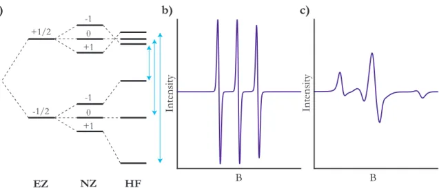
-1/2 +1/2 -1 +1 0 -1 +1 0 EZ NZ HF a) b) c) B B Int ensit y Int ensit y

Figure 2.2: Energy levels in nitroxide radicals. a) The electron’s energy is split by the electron Zeeman (EZ) and the nuclear Zeeman (NZ) interaction, giving rise to 6 energy levels. These are modulated by the hyperfine (HF) interaction, as well as several others that minorly change energy levels. Due to momentum

conservation, only 3 energetic transitions occur, giving rise to the 3 peaks shown in (b). b-c) Simulated EPR spectra for nitroxide radicals near the isotropic limit (b) and the rigid limit (c). Each spectrum contains 3 peaks, though these are more easily distinguished in the isotropic limit, where peaks are narrower and do not overlap.

high concentrations of spin-labels, resulting in spectral broadening. It may also be exploited, by intentionally introducing multiple probes into the same molecule in order to deduce the distances between them. The EE Hamiltonian is given by:

HEE = S𝑇1JS2 (2.5)

J describes the total interaction between the two spins. By specifically studying the dipole-dipole (DD) interaction between these two probes and simplifying, we can express this Hamiltonian (HDD) in terms of the distance vector (r12) between the two

spins: HDD = S𝑇1JS2 (2.6) = 𝜇0𝜇 2 𝐵𝑔1𝑔2 4𝜋~ 1 𝑟3 12 [︂ S𝑇₁S2− 3 𝑟2 12 (S𝑇₁r12)(S𝑇2r12) ]︂ (2.7)

(27)

Because the energy varies approximately with probe-probe according to 𝑟−3

12,

exper-imentalists can exploit this relationship to determine the distribution of 𝑟12 using

pulsed EPR methods like DEER or DQC. This gives data analogous to data collected from Förster resonance energy transfer (FRET) experiments, but with physically smaller probes.

2.1.1 Continuous-wave electron paramagnetic resonance

the-ory

Today, one of the primary uses of CW-EPR is the study of dynamic behavior in spin-labeled samples. The principle is straight-forward: the shape of an observed EPR spectrum depends on the average rate of rotational diffusion of an observed probe, as well as several energetic parameters. EPR is sensitive to diffusion over a broad range of correlation times (𝑡𝑅= 10−12 s in the fast motion limit to 𝑡𝑅 = 10−6 s in the

slow motion limit)64_{, making it a very robust measurement tool. The range itself can}

be further subdivided, based on the type of model appropriate for spectral fitting. Dynamics for virtually all spin-labeled macromolecules fall within the slow-motional regime (with correlation times ranging from 𝜏𝑅 = 10−6 s to 𝜏𝑅 = 10−9 s), which

requires the most challenging theoretical treatment.

In the slow-motion regime, which corresponds to dynamic fluctuations in chain position, continuous wave electron paramagnetic resonance (CW-EPR) spectra follow the stochastic Liouville equation:

𝐼(𝜔 − 𝜔0) = 1 𝜋 ⟨⟨ 𝑣 ⃒ ⃒ ⃒[(˜Γ − 𝑖 ˜H + 𝑖(𝜔 − 𝜔0)𝐼] −1⃒_⃒ ⃒𝑣 ⟩⟩ (2.8) In this equation, 𝐼 represents the spectral intensity as a function of angular mi-crowave frequency (𝜔) relative to some reference frequency (𝜔0), represents a

start-ing vector that already contains the spin operator and the statistical distribution of up/down spins, ˜Γ represents the symmetrized diffusion superoperator, ˜H represents the Liouville superoperator, and 𝑖 represents the imaginary unit. Given a set of pa-rameters c = {𝑐1, 𝑐2, · · · , 𝑐𝑛} describing our experiment, we may solve this equation

(28)

numerically with high computational efficiency. Freed derived and implemented this approach in 1976, and his original solution remains central to most CW-EPR analysis tools.64–68

The precise number and definition of the parameters studied depends on the degree of detail that the user needs, but typically they include the hyperfine tensor (A), the tensor of electron 𝑔 values (g), the rotational diffusion tensor (DR, which is generally

expressed in terms of a tensor of rotational correlation times, 𝜏R, or in terms of the

base 10 logarithm of tensor components, ¯R). Since each of these tensors is real-symmetric, they may be expressed in terms of 3 axial components. For instance:

A = ⎡ ⎢ ⎢ ⎢ ⎣ 𝐴𝑥𝑥 0 0 0 𝐴𝑦𝑦 0 0 0 𝐴𝑧𝑧 ⎤ ⎥ ⎥ ⎥ ⎦ (2.9)

Similarly, g may be resolved into 𝑔𝑥𝑥, 𝑔𝑦𝑦 and 𝑔𝑧𝑧, and ¯R may be resolved into

𝑅𝑥𝑥, 𝑅𝑦𝑦 and 𝑅𝑧𝑧. Because the model involves relativistic rotations between frames,

a director angle (𝜓), which describes spin orientation, and a set of Euler angles (𝛼,𝛽 and 𝛾) are also involved. Additional line-broadening parameters are also frequently included.

One assumption of this classical model is that spins are uniformly distributed in the director frame. When this assumption fails, as often happens in real systems, more complex models are needed. For these cases, researchers typically turn to two more-detailed models: the macroscopic order, microscopic disorder (MOMD) model, where spectra are generated for a variety of orientations and then composed into a single spectrum; and the slowly relaxing local structure (SRLS) model, which generalizes this idea to allow time-dependent variation in the area of locally-ordered region. Because SRLS requires higher-frequency measurements, MOMD calculations are more common.

These models make the CW-EPR spectra of radicals in the slow-motional regime computable. However, in order to truly make use of these insights, we need to reverse-engineer them, using non-linear fitting, a process where the deviation between

(29)

exper-imental data and a model is minimized as a function of important fit parameters. (For further details, refer to Section 2.1.3.) In practice, this only works well when varying a small number of parameters. Generally, if we tried to optimize over all 15+ of the parameters mentioned in this section, we could expect the fitting process to become difficult and unreliable – either because local minima of the error function would become too common, or because we would identify so many high-quality fits that it would be impossible to select the physically accurate one.

For these reasons, we make several assumptions that reduce the size of our pa-rameter space. First, based on the experimental setup, we note that most of the angles are known so we can use trusted default values. Second, we note that the A and g tensors are independent from the diffusion rate, and can be established by freezing a sample and fitting its rigid-limit spectrum (which has the benefit of being far less computationally intensive than fits in the slow-motional regime). If further simplification is needed, we can reduce the complexity of A and g by assuming that 𝑔𝑥𝑥 = 𝑔𝑦𝑦 = 𝑔⊥ (in this notation 𝑔𝑧𝑧 = 𝑔‖) and 𝐴𝑥𝑥 = 𝐴𝑦𝑦 = 𝐴⊥. Finally, we can

(and typically do) assume that rotational diffusion occurs much more rapidly around one axis than any of the others, allowing us to rely on a single diffusion parameter 𝑅 = log(𝐷𝑅).69 In practice, these assumptions allow us to reliably fit spectra using

as few as 3-4 fit parameters – a much more manageable optimization problem.

Today, most researchers use Freed’s NLSL package or Stoll’s EasySpin package for this process.66,67 _{NLSL contains a high-efficiency implementation of the}

Levenberg-Marquardt minimization algorithm, but uses a Fortran 77 command-line utility rather than a callable function. This makes it difficult to script. EasySpin contains a MatLab wrapper for NLSL. However, it ignores higher order contributions to spectral broad-ening, and it does not allow users to vary every the parameter accessible in NLSL. Both EasySpin and NLSL operate by performing nonlinear fitting of experimental spectra. The details of this procedure are described Section 2.1.3.

(30)

2.1.2 Pulsed dipolar spectroscopy

Given a molecule containing two spin-labels, pulsed EPR measurements allow us to extract the distance distribution between them (effectively, a pair-distribution func-tion). This enables scientists to make direct distance measurements in spin-labeled molecules. When a pair of spins are close together (and thus have a strong dipo-lar coupling) the dipole-dipole interaction may affect a CW-EPR spectrum – how-ever, over the longer distances (> 1.5 nm) that typically interest spectroscopists, this component is week, and can generally only be detected using Fourier-transform methods.70–73 _{By using this family of techniques, generally called pulsed dipolar}

spec-troscopy (PDS) techniques, it is possible to gain insight into the structure of proteins and other macromolecules, in much the same way that fluorescence spectroscopists use FRET experiments.

As explained in Section 2.1, pairs of spins experience an electron dipole-dipole cou-pling that strengthens as the distance between them shrinks. By exciting the sample with a controlled sequence of microwave pulses designed to suppress the hyperfine interaction, we become particularly sensitive to this energetic contribution, allowing us to determine the inter-spin distance of a pair of spins (see Equation 2.7). The most common technique for this is double electron-electron resonance (DEER), also known as pulsed electron-electron double resonance (PELDOR). In this experiment, we typically use 4 pulses, applied in a particular time sequence, in order to determine interprobe distances. The method works best for distances between 1.5 and 8 nm. In this work, I also employed double quantum coherence (DQC) experiments, which work similarly, but are sensitive to smaller inter-probe distance distributions.74,75

These distributions are then fit using Tikhonov regularization, an optimization algo-rithm that imposes reasonable constraints (i.e. a degree of smoothness) on the shape of the inter-probe distribution.

(31)

2.1.3 Nonlinear Fitting of EPR Spectra

This approach aims to minimize the deviation of a model spectrum 𝐼(𝜔 −𝜔0, c), from

an experimental spectrum, 𝐼𝑒𝑥𝑝(𝜔 − 𝜔0), as a function of the experimental parameters

c. We represent this by the 𝜒2 function: 𝜒2(c) = 𝑛 ∑︁ 𝑖=1 [𝐼(𝜔𝑖 − 𝜔0, c) − 𝐼𝑒𝑥𝑝(𝜔𝑖− 𝜔0)]2 𝜎2 𝑖 (2.10) In this equation, 𝜎2

𝑖 represents the individual uncertainty in 𝐼𝑒𝑥𝑝(𝜔𝑖− 𝜔0) at each

point 𝑖. In general, 𝜒2 is non-convex, meaning that it may possess many disconnected

local minima. In such cases, we must rely on numerical methods to identify the opti-mal set of parameters, c*_{, that describe the spectrum. Below, I provide an overview}

of common methods for fitting.

Grid-Search Optimization

In this approach, we overlay a grid of points upon the c parameter space and choose the point producing the best 𝜒2 _{value. This method exists in both NLSL and}

EasySpin, but is very inefficient.

Monte Carlo Optimization

This approach resembles grid-search optimization, except that we choose points ran-domly from within the parameter space. In low-dimensional parameter spaces, this is marginally efficient than grid-search; however, it becomes more efficient when the dimension of c increases. This method is only implemented in EasySpin.

Levenberg-Marquardt Optimization

This algorithm uses a gradient-descent method designed specifically for curve-fitting problems. In this process, users provide an initial guess value, c0, and the algorithm

iteratively steps along the negative gradient of 𝜒2 _{until reaching a local minimum.}

Adaptations exist to enable bounded optimization, but typically this algorithm is used in an unbounded fashion. The algorithm typically obtains linear convergence

(32)

(which means that the difference between 𝜒2 _{at the 𝑛}th _{iteration and 𝜒}2 _{at the}

op-timum, 𝜒2_(c

n) − 𝜒2(c*), decreases at a rate proportional to 𝑒−𝑛. It is well-suited to

most problems where 𝜒2 _{is convex. However, when 𝜒}2 _{is not a convex function, the}

algorithm requires a lucky initial guess to reach the global minimum. In the case of typical EPR spectra, random initial guesses rarely reach the global minimum of 𝜒2_.

Both NLSL and EasySpin enable Levenberg-Marquardt optimization.

By establishing reasonable physical bounds, we can adapt Levenberg-Marquardt optimization for global optimization by employing a Monte Carlo or grid-search ap-proach to selecting c0 values. By selecting a randomized sequence of initial guesses

and starting the Levenberg-Marquardt algorithm from each of these, we become likely to identify the global optimum within the bounds. A grid-search approach to picking c0 will also work. Neither NLSL nor EasySpin implements these variants, despite

their comparatively rapid convergence rates in CW-EPR spectral analysis.

Particle-Swarm Optimization

In particle swarm optimization, a selection of ’particles’ receive initial positions and random velocities within the problem space. Then, each particle moves according to its velocity. The position of each particle updates to the best position it has found, and the particle receives a new, randomized velocity. This process iterates until reaching a convergence criterion, at which point the algorithm has reached the global minimum. The method makes no assumptions of differentiability and does not require gradient calculations, making it useful in cases where 𝜒2 is highly multimodal, as is

often the case in EPR spectral fitting. Particle swarm optimization tends to be quite robust, generally identifying the optimum of 𝜒2, even in parameter spaces of fairly

high dimension. For EPR fitting, particle swarm optimization is only implemented in EasySpin.

Simulated Annealing

Like particle swarm optimization, simulated annealing provides robust global fitting. In a basic iteration, the program probabilistically chooses whether to remain in its

(33)

current state or to move to a nearby state, based on the value of 𝜒2 _{in both states.}

Changes that reduce 𝜒2 are always accepted, and changes that increase 𝜒2 are

ac-cepted with a probability that depends upon the ’temperature’ of the system. Over time, the ’temperature’ of the system is slowly reduced. In this way, the algorithm explores a large fraction of parameter space before cooling to a minimum value. This helps to ensure global convergence. Neither NLSL nor EasySpin currently employs this optimization protocol, despite its popularity in the broader curve-fitting commu-nity.

2.2 Flow synthesis of peptides

In general, I synthesized the peptides presented in this thesis using the flow-synthesis methods developed in the Pentelute group.76 _{The advantages of this approach over}

conventional solid state peptide synthesis include high speed (each coupling takes approximately 1 minute) and high synthetic yield. Briefly, a sample of H-rink amide resin is prepared in a syringe and swelled in N -N dimethylformamide (DMF). First, the resin is washed with DMF at the desired temperature generally 90 ∘_{C. Then,}

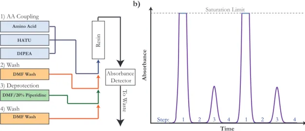
in turn it is: 1) washed with a solution containing an Fluorenylmethyloxycarbonyl-(Fmoc-) protected amino acid and activating agents; 2) washed with more DMF; 3) washed with a solution of DMF-20% piperidine to remove the Fmoc, leaving an exposed amine; and 4) washed again with DMF. The result is a resin that is covalently bound to the C-terminus of an amino acid. With the molecule’s N-terminus free, steps 1-4 can now be run again, with a new amino acid. Downstream, an absorbance detector provides information about the quality of the synthesis. A schematic of this process, and of the expected absorbance profile, is shown in Figure 2.3.

By iteration, sequences of high length and purity can be synthesized, provided that the per-step yield remains very high. To spin-label our sequences, we incorporated TOAC (Fig. 2.1) directly into their backbone, substituting it for an amino acid of choice. While theoretically TOAC can be attached like any other amino acid (Fmoc-TOAC is commercially available) the molecule’s rigid and bulky structure makes this

(34)

Amino Acid HATU DIPEA DMF Wash DMF/20% Piperidine DMF Wash R esin T o W aste 1) AA Coupling 2) Wash 4) Wash 3) Deprotection Absorbance Detector Absorbance Time 1 2 3 4 1 2 3 4 Step: a) b) Saturation Limit

Figure 2.3: Peptide flow synthesis schematic. a) The four flow-steps that are iterated to attach each consecutive amino acid to the resin. b) A diagrammed absorbance profile of the attachment of 4 amino acids. Fmoc is UV-active, so in Step 1, the high concentration of reactants overwhelms the detector. In Step 3, the profile of Fmoc deprotection products is observed. In the wash step, signal vanishes because DMF is not active at this wavelength.

process challenging, a difficulty I overcame in Chapter 3.

2.3 Liquid Chromatography Techniques

Molecules including those synthesized according to Section 2.2 typically require char-acterization and purification before use. In general, peptide-based samples in this paper were characterized by reverse-phase liquid chromatography mass spectrometry (LC-MS) in order to determine their purity. In this technique, samples are suspended in a mixture of water, acetonitrile and a dilute additive (typically formic acid for LC-MS) to control pH and promote solubility. Then, a small quantity is loaded onto a column – typically a C3 or C18 column – and a water:acetonitrile gradient is used to separate distinct chemical components by their polarity. Upon reaching the end of the column, the solution is then injected into a mass-spectrometer, where the charge:mass ratio of the solute can be studied to determine its molecular weight. I used LC-MS to identify compounds of interest for subsequent purification, to verify the quality of purified products, and to quantify reaction yields.

(35)

To purify samples, I used high performance liquid chromatography (HPLC), which works very similarly. A solution of water, acetonitrile and dilute trifluoroacetic acid was used to dissolve a crude product, which was then loaded onto a preparatory HPLC column and separated by a water:acetonitrile gradient. Using UV and mass-spectrometric intensity of the eluted product, I could separate the important com-pounds from impurities by identifying and isolating the product-peak.

2.4 Flow cytometry

In this technique, specially prepared cell cultures are loaded onto a fluorescence detec-tor. Fluorescently-labeled macromolecules are flowed over the cultures, so that adhe-sion can be detected by a fluorescence measurement. By varying the concentration of the macromolecule, we can establish the binding constant of the macromolecule. Sim-ilarly, by measuring fluorescence between a fixed concentration of the macromolecule and a varying concentration of competing analogues, we can compare the viability of those analogues quantitatively, using the half-maximal inhibitory concentration (IC50) – the competitor concentration required to inhibit 50% of the binding of the fluorescent molecule. Thus, compounds which more effectively bind to cells will have a lower IC50 than compounds which bind less effectively, since it will take a lower concentration to displace the fluorophor.

2.5 Molecular dynamics

In this work, I occasionally studied short molecular dynamics simulations of peptides in order to gain insight into their secondary structure. In order to prepare initial struc-tures, I used the Pep-Fold 3 algorithm to predict an energetically favorable starting conformation, and ran brief simulations using the CHARMM36 force field in Gro-macs. Using Gromacs algorithms, I computed hydrogen bonding maps, secondary structure maps, distance distributions, and assorted other data for comparison with EPR results.

(36)

(37)

Chapter 3 Quantifying residue-specific

conformational dynamics of a highly

reactive 29-mer peptide

This chapter was adapted from the publication "Quantifying residue-specific conforma-tional dynamics of a highly reactive 29-mer peptide", originally published in Scientific Reports.77

3.1 Abstract

Understanding structural transitions within macromolecules remains an important challenge in biochemistry, with important implications for drug development and medicine. Insight into molecular behavior often requires residue-specific dynamics measurement at micromolar concentrations. We studied MP01-Gen4, a library pep-tide selected to rapidly undergo bioconjugation, by using electron paramagnetic res-onance (EPR) to measure conformational dynamics. We mapped the dynamics of MP01-Gen4 with residue-specificity and identified the regions involved in a structural transformation related to the conjugation reaction. Upon reaction, the conformational dynamics of residues near the termini slow significantly more than central residues, indicating that the reaction induces a structural transition far from the reaction site.

(38)

Arrhenius analysis demonstrates a nearly threefold decrease in the activation energy of conformational diffusion upon reaction (8.0 𝑘𝐵𝑇 to 3.4 𝑘𝐵𝑇), which occurs across

the entire peptide, independently of residue position. This novel approach to EPR spectral analysis provides insight into the positional extent of disorder and the nature of the energy landscape of a highly reactive, intrinsically disordered library peptide before and after conjugation.

3.2 Introduction

Combinatorial, library-based strategies for discovering functional peptides have trans-formed biochemistry, enabling tremendous improvements in enzyme design, disease diagnosis, and drug development.78_{One prototypical example of sequences identified}

by combinatorial discovery is the family of MP peptides – molecules selected to un-dergo nucleophilic aromatic substitution (S𝑁Ar) reactions via a single cysteine residue

(Fig. 3.1).79–81 _{Their mild reaction conditions make reactive MP peptides optimal}

for bioconjugation82–84 _{while preserving orthogonality to other popular conjugation}

methods including click chemistry85–87_{, protein-facilitated approaches (such as the}

biotin-streptavidin interaction)88–92_{, and the use of peptide tags.}93–96 _{Bioconjugation}

tools have become essential technology, enabling controlled coupling of biomolecules for important diagnostic and therapeutic purposes. In the case of MPs, many features of their backbone dynamics and conformational behavior remain unknown because the residue-specific measurements required are difficult to achieve at low (𝜇M) con-centrations.79–81

Here we investigate MP01-Gen4, an abiotic 29-mer selected from among 5 x 1013 randomized peptides and subsequently optimized via experimental and computational methods.79,81_{The resulting sequence reacts rapidly with perfluoroarenes,}

demonstrat-ing quantitative conversion in under five minutes (Fig. 1). Previously reported circu-lar dichroism (CD) measurements show experimentally that MP01-Gen4 undergoes a random-coil-to-helix structural transformation upon interaction with a perfluoroarene probe.81,97 _{Calculations from the PrDOS intrinsic disorder prediction tool suggested}

(39)

Figure 3.1: The MP01-Gen4 peptide reacts rapidly with a perfluoroarene capture agent (CA) via nucleophilic aromatic substitution (S𝑁Ar) to

form the complex MP01-CA in approx. 5 mins. The peptide backbone’s dynamic structure (illustrated here as a cartoon) is related to the high reactivity of MP01-Gen4 with perfluoroarenes.

disorder in residues 1-7 and 24-29, and predictions using Rosetta software suggest the existence of transient 𝛼-helix-like order in residues near the center of the peptide, prior to S𝑁Ar reaction.81Circular dichroism studies demonstrate that the peptide increases

in helical content upon reaction, but neither these experiments nor PrDOS/Rosetta predictions could identify the residues involved. Thus, experimentally identifying the residues involved in this transition, and understanding the extent to which distinct regions of the sequence exhibit disorder or flexibility, is important for understanding the behavior of MP01-Gen4. Although this type of structural transition is common among natural sequences, its emergence from a library of abiotic peptides in the con-text of a non-biological reaction is noteworthy.47–49_{We aimed to identify the residues}

involved in this structural transition and to understand the relationship between the dynamic behavior of MP01-Gen4 and its structural transition.81

Conformational studies of peptides typically require residue-specific insight into dynamics. We acquired this information by introducing radical electron spin-labels at specific residues of MP01-Gen4 and performing electron paramagnetic resonance (EPR) spectroscopy to obtain rotational diffusion coefficients (inversely related to

(40)

3260 3300 3340 7 8 9 1 2 3 4 5 200 220 240 260 2 Fast Frozen a) b) c) d) T=308 K T=281 K N O H2N COOH H2N COOH

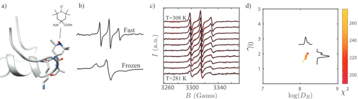
Figure 3.2: Experimental approach to dynamics measurements. a) TOAC is embedded along the MP01-Gen4 backbone. b) EPR line shapes of a TOAC-labeled MP01-Gen4 peptide at 308 K (top) and 150 K (bottom) indicate fast and slow rate of motion, respectively. c) EPR spectra are fit for rotational diffusion rate at

different temperatures. d) The fitting function (𝜒2_{) represents deviation between}

experimental data and a fitting model. Optimal values for fit parameters such as the log of the rotational diffusion coefficient (log (𝐷𝑅)) and the Gaussian line-broadening

(𝛾0) are extracted from clusters of good fits near the global minimum of 𝜒2.

rotational correlation times) of the spin-label’s motion.65–67,98 _{This motion primarily}

originates from conformational changes of the backbone, and its timescale depends on position, since more flexible regions of a peptide change conformation more rapidly.99

We can therefore use this approach to map the flexibility of a sequence with residue-level resolution, even at micromolar concentrations.3,58,68,100–104

3.3 Experimental Methods

The basic methodology of our experiments is outlined in Fig. 3.2. In brief, we used TOAC (TOAC = 2,2,6,6-tetramethylpiperidine-N -oxyl-4-(9-fluorenyl methyloxy carbonyl-amino)-4-carboxylic acid) to spin-label each peptide (Fig. 3.2a) and mea-sured its EPR spectrum. The line shapes of the spectra encode dynamics information (Fig. 3.2b). We fit our measurements at each probe position at ten temperatures, ranging from 280 K to 308 K (Fig. 3.2c), and measured distributions of good fits in order to quantify uncertainty (Fig. 3.2d). This strategy enabled rotational diffusion rate, 𝐷𝑅, measurements at each site and temperature.

Ten MP01 variants were selected, with TOAC positions chosen to provide approx-imately regular spacing, by a systematic scan of alanine substitutions, which we used

(41)

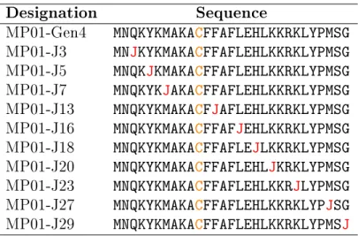
Table 3.1: Names and sequences of the MP01-Gen4 variants employed in this study. J is the amino acid spin-label TOAC; Cis the reactive cysteine.

Designation Sequence

MP01-Gen4 MNQKYKMAKACFFAFLEHLKKRKLYPMSG MP01-J3 MNJKYKMAKACFFAFLEHLKKRKLYPMSG MP01-J5 MNQKJKMAKACFFAFLEHLKKRKLYPMSG MP01-J7 MNQKYKJAKACFFAFLEHLKKRKLYPMSG MP01-J13 MNQKYKMAKACFJAFLEHLKKRKLYPMSG MP01-J16 MNQKYKMAKACFFAFJEHLKKRKLYPMSG MP01-J18 MNQKYKMAKACFFAFLEJLKKRKLYPMSG MP01-J20 MNQKYKMAKACFFAFLEHLJKRKLYPMSG MP01-J23 MNQKYKMAKACFFAFLEHLKKRJLYPMSG MP01-J27 MNQKYKMAKACFFAFLEHLKKRKLYPJSG MP01-J29 MNQKYKMAKACFFAFLEHLKKRKLYPMSJ

to identify locations where modifications would minimally perturb the reactivity of the peptide. In a two positions (5 and 7) we were willing to replace residues known to be important for reactivity, on the basis that we didn’t want to replace nearby charged residues. Sequences and designations are reported in Table 3.1.

3.3.1 Materials

1-[Bis(dimethylamino)methylene]-1H-1,2,3-triazolo[4,5-b]pyridinium 3-oxid hexafluo-rophosphate (HATU), Fmoc-L-Ala-OH, Fmoc-L-Cys (trt)-OH, Fmoc-L-Glu (tBu)-OH, Fmoc-L-Phe-(tBu)-OH, Fmoc-Gly-(tBu)-OH, Fmoc-L-His (Boc)-OH Fmoc-L-Lys (Boc)-(tBu)-OH, Leu-OH, Met-OH, Asn (Trt)-OH, Pro-OH, Fmoc-L-Gln (Trt)-OH, Fmoc-L-Arg (Pbf)-OH, Fmoc-L-Ser (tBu)-OH, Fmoc-L-Tyr (tBu)-OH and Fmoc-TOAC-OH were purchased from Chem-Impex International. H-rink-amide ChemMatrix Hyr resin was obtained from PCAS BioMatrix, Inc. (7-Azabenzotriazol-1-yloxy)tripyrrolidino phosphonium hexafluorophosphate (PyAOP) was purchased from P3 BioSystems. N,N-dimethylformamide (DMF), acetonitrile (ACN) and di-ethyl ether were purchased from VWR (Radnor, PA). N,N-diisopropyldi-ethylamine (DIPEA), formic acid (FA), 10x phosphate buffered saline (PBS), trifluoroacetic acid (TFA) and triisopropylsilane (TIPS) were obtained from Sigma-Aldrich. Potassium hexaferrocyanate (III) (K3Fe(CN)6) was purchased from Alfa-Aesar.

(42)

Alltech low pressure polytetrafluoroethane (PTFE) tubing and Leica BioSystems Crytoseal capillary tube sealant were purchased from Fisher-Scientific. Liquid ni-trogen was purchased from Airgas. Wilmad 4x250 mm quartz glass EPR tubes were purchased from Cambridge Isotope Laboratories. Water (18.2 MΩ) was purified using a Milli-Q Direct 8 system.

3.3.2 TOAC Peptide Synthesis

Peptides and the perfluoroarene capture agent (CA) were synthesized according to literature, using ChemMatrix H-rink amide resin (0.49 meq/g) on the 0.1 mmol scale.76,79 _{Flow-synthesis of standard amino acids uses a DMF solution of 0.2 M}

amino acid, 0.17 M activating agent and 5% (v/v) DIPEA flushed over the sample at 80 mL/min for 15 s, followed by DMF washing and deprotection using DMF 20% piperidine. TOAC was coupled using 50 mM Fmoc-TOAC, 47.5 mM HATU, and 10% DIPEA at a rate of 40 mL/min for 15 s, followed by the usual washing and Fmoc-deprotection steps. Due to steric limitations of the TOAC, the kinetics of cou-pling natural amino acids to resin-bound TOAC proved to be exceptionally slow. To bypass this problem, we couple the sterically-hindered post-TOAC residue using 0.2 M amino acid, 0.14 M activating agent and 10% DIPEA pumped at 10 mL/min for 10 min, followed by the usual wash and deprotection steps. All subsequent residues were coupled normally. Completed peptides were cleaved for 2 h at RT using (90% TFA, 5% water, 5% TIPS v/v), a cleavage cocktail for TOAC peptides.40 The result-ing peptides were then precipitated and washed 3x in diethyl ether (-80 ∘_{C), before}

drying under vacuum. The dried product was dissolved and purified by reverse phase high performance liquid chromatography (HPLC). Synthetic yields for each peptide, calculated from the crude mass collected, are reported in Table 3.2.

3.3.3 LC-MS Analysis

The purity of all peptides was analyzed by liquid chromatography mass spectrometry (LC-MS) using an Agilent 6520 ESI-Q-TOF mass spectrometer. For convenience,

(43)

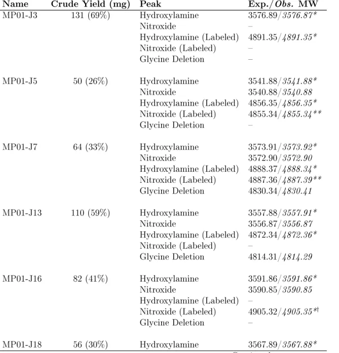
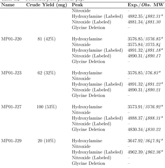
Table 3.2: Crude yields and LC-MS data for MP01-Gen4 variants.Crude yields (mg) are reported for each peptide (column 2), along with masses

expected/observed for the peaks present in the LC-MS traces in Figures 3.3 and 3.4. In most cases, hydroxylamine signal is dominant, due to reduction of the nitroxide in acidic conditions before/during the LC-MS scan. A minor peak, corresponding to the nitroxyl version of the C-terminal glycine deletion product, appeared in a few spectra – however, this is always a minority product and probably had a negligible impact on EPR analysis. Observed masses are calculated using the [M+3H]3+

charge state for the unlabeled peptides, and the [M+4H]4+ charge state for the

labeled peptides. MS data are reported in Appendix B.

Name Crude Yield (mg) Peak Exp./Obs. MW

MP01-J3 131 (69%) Hydroxylamine 3576.89/3576.87* Nitroxide – Hydroxylamine (Labeled) 4891.35/4891.35* Nitroxide (Labeled) – Glycine Deletion – MP01-J5 50 (26%) Hydroxylamine 3541.88/3541.88* Nitroxide 3540.88/3540.88 Hydroxylamine (Labeled) 4856.35/4856.35* Nitroxide (Labeled) 4855.34/4855.34** Glycine Deletion – MP01-J7 64 (33%) Hydroxylamine 3573.91/3573.92* Nitroxide 3572.90/3572.90 Hydroxylamine (Labeled) 4888.37/4888.34* Nitroxide (Labeled) 4887.36/4887.39** Glycine Deletion 4830.34/4830.41 MP01-J13 110 (59%) Hydroxylamine 3557.88/3557.91* Nitroxide 3556.87/3556.87 Hydroxylamine (Labeled) 4872.34/4872.36* Nitroxide (Labeled) – Glycine Deletion 4814.31/4814.29 MP01-J16 82 (41%) Hydroxylamine 3591.86/3591.86* Nitroxide 3590.85/3590.85 Hydroxylamine (Labeled) – Nitroxide (Labeled) 4905.32/4905.35*† Glycine Deletion – MP01-J18 56 (30%) Hydroxylamine 3567.89/3567.88* Continued on next page

(44)

Table 3.2 – Continued from previous page

Name Crude Yield (mg) Peak Exp./Obs. MW

Nitroxide – Hydroxylamine (Labeled) 4882.35/4882.31* Nitroxide (Labeled) 4881.34/4881.30 Glycine Deletion – MP01-J20 81 (42%) Hydroxylamine 3576.85/3576.85* Nitroxide 3575.84/3575.84 Hydroxylamine (Labeled) 4891.32/4891.18* Nitroxide (Labeled) 4890.31/4890.17 Glycine Deletion – MP01-J23 62 (32%) Hydroxylamine 3576.85/576.83* Nitroxide – Hydroxylamine (Labeled) 4891.32/4891.22* Nitroxide (Labeled) 4890.31/4890.21 Glycine Deletion – MP01-J27 100 (53%) Hydroxylamine 3573.91/3576.92* Nitroxide – Hydroxylamine (Labeled) 4888.37/4888.31* Nitroxide (Labeled) – Glycine Deletion 4830.34/4830.22 MP01-J29 20 (10%) Hydroxylamine 3647.92/3647.94* Nitroxide – Hydroxylamine (Labeled) 4962.39/4962.36* Nitroxide (Labeled) – Glycine Deletion –

* This is the principle peak observed in the LC-MS traces shown in Figures 3.3 and 3.4

** The nitroxide LC-MS trace overlaps the hydroxylamine trace, but appears to be the minor product.

† _{In all but this case, the primary product contains the hydroxylaminated version}

of the TOAC residue, due to reducing conditions prior to/during loading onto the LC-MS column. In this case, the true nitroxide form (which differs by the mass of an H1 atom) dominated – either because the sample was loaded relatively quickly or because proximity to the labeled cysteine more effectively protected this nitroxyl radical from reduction.

(45)

solutions A and B are defined as follows: A – water, 0.1% formic acid; D – acetonitrile, 0.1% formic acid. LC-MS was carried out according to the following steps: in the range of 0-2 min, a 95% A - 5% B wash; in the range of 2-11 min, a 5-65% B linear ramp; and in the range of 11-12 min, a 65% B. We used a flow rate of 0.8 mL/min on a Zorbax 300SB C3 column (2.1 x 150 mm, 5 𝜇m), at 40 ∘_{C. MS was performed by}

positive electrospray ionization (ESI). Observed masses were reported by averaging the major peak in the total ion current (TIC).

3.3.4 Preparative HPLC

Crude peptides were purified by reverse phase high performance liquid chromatogra-phy (HPLC). Solutions C and D are defined as follows: C – water, 0.1% trifluoroacetic acid; D – acetonitrile, 0.1% trifluoroacetic acid. Peptides were dissolved in 50% C, 50% D and loaded onto an Agilent Zorbax C3 column (21.2 x 250 mm, 7 𝜇m). HPLC was carried out at a flow rate of 5 mL/min according to the following steps: in the range of 0-5 minutes, a 95% C – 5% D wash; in the range of 5-80 min, a 5-45% C linear ramp; and in the range of 80-85 min, a 45% C wash.

3.3.5 EPR Sample Preparation

All EPR samples were prepared by injecting 10 𝜇L solutions of peptide in 1x phos-phate buffer solution (PBS) at a concentration of 45 𝜇M into a PTFE capillary tubes, sealed with Crytoseal resin. S𝑁Ar reactions were performed at 45 𝜇M peptide

concentration in PBS at RT for 15 min, with CA in 5x molar excess. Potassium hexacyanoferrate(III) (K3Fe(CN)6) was added to all samples before EPR analysis to

reverse the reduction of nitroxides by TFA. The maximum K3Fe(CN)6 concentration

that did not result in detectable peptide degradation was used in each case, and no subsequent purification efforts were made since neither unreacted hydroxylamines nor K3Fe(CN)6 interfere with the nitroxide EPR signal. The elution profiles are reported

in Fig. 3.3 (before conjugation) and Fig. 3.4 (after conjugation), with all peaks la-beled. By comparing integrated intensity of the unreacted peptide elution peak in

(46)

each profile, we computed the reaction S𝑁Ar yields reported in Fig. 3.5. In the case

of unreacted peptides, 0.2 equiv. K3Fe(CN)6 was used for all analysis. In the case of

the reacted peptides, 1 equiv. K3Fe(CN)6 was used for all analysis. The exception

in both cases was the sequence MP01-J29. This peptide is less stable in the presence of K3Fe(CN)6, so none was added to unreacted MP01-J29 and 0.2 equiv. were used

for EPR analysis of the reacted peptide. The reduction of the nitroxide in MP01-J29 increased the uncertainty of the fit of unreacted MP01-J29. After EPR, each sample was recovered and analyzed by LC-MS.

3.3.6 EPR Experiments

Continuous wave electron paramagnetic resonance (CW-EPR) spectra were collected at X-band (9.43 GHz) using a Bruker EMX+ with a variable temperature unit. Spec-tra were collected over 150 G field sweep with center field at 𝐵 = 3315 G, with atten-uation of 15 dB and modulation amplitude of 1.5 G. EPR spectra of a background sample containing only PBS and K3Fe(CN)6 were subtracted from each peptide

spec-trum. Variable temperature spectra of each sample were collected in the range of 275-310 K, in increments of 5 K. We verified by LCMS that each peptide was undam-aged by the heating process and that they reacted completely with the perfluoroarene target, demonstrating that their functionality was retained.

3.3.7 EPR Fitting

Initial fitting of each sample at 150 ∘_{C was carried out to determine hyperfine A}

and electron g tensors using the pepper function in Easyspin.67 _{Since frozen spectra}

were identical under scaling, regardless of the position of TOAC, the fitted tensor components of 𝑔𝑥𝑥 = 2.0081, 𝑔𝑥𝑥 = 2.0051, 𝑔𝑥𝑥 = 2.0020, 𝐴⊥= 5.13 G and 𝐴‖ = 37.6

G were assigned to all samples during EPR fitting at higher temperatures.

Analyses of higher-temperature EPR data were carried out using non-linear least squares analysis via the NLSL program to perform Levenberg-Marquardt curve-fitting.66,67 _{We fit the data for the base 10 logarithm of rotational diffusion rate,}

(47)

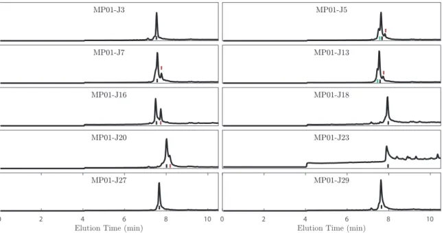
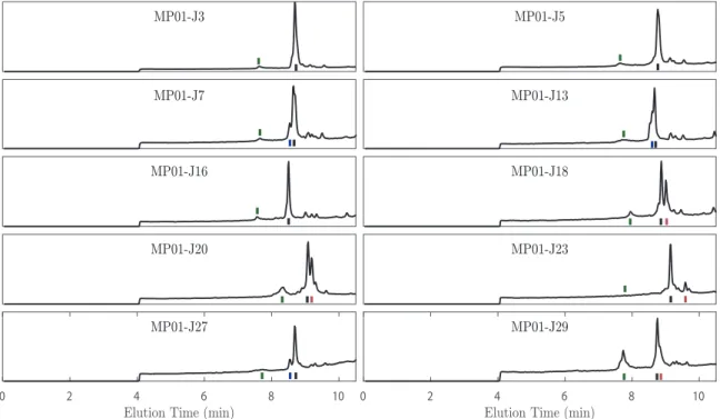
0 2 4 6 8 10 0 2 4 6 8 10

Figure 3.3: LC-MS elution profiles of MP01-Gen4 variants before S𝑁Ar

reaction and after EPR analysis. Since the samples were diluted in a solution containing TFA, and because the LC-MS column contains FA, the product often appears in both its nitroxyl and its hydroxylamine forms, and these are marked by red and black lines, respectively. The presence of a small dimer peak was usually noted. This is marked by a green line when separate from the principle peak. Reaction yields were estimated by comparing the integrated peak intensities of the unreacted species shown here (via integration/addition of both hydroxylamine and nitroxyl peaks) and after undergoing reaction (Fig. 3.4).

(48)

0 2 4 6 8 10 0 2 4 6 8 10

Figure 3.4: LC-MS elution profiles of the MP01-Gen4 variants following S𝑁Ar reaction and EPR analysis. Since the samples were diluted in a solution

containing TFA, and because the LC-MS column contains FA, the product often appears in both its nitroxyl and its hydroxylamine forms, and these are marked by red and black lines, respectively. The unreacted peptide peak is marked with a green line. Reaction yields were estimated by comparing the integrated peak intensities of the unreacted species shown here (via integration/addition of both hydroxylamine and nitroxyl peaks) and the same peak prior to reaction (Fig. 3.3). In MP01-J7, -J13 and -J27, a minor glycine deletion product was noted (blue) that is invisible in the elution profiles prior to S𝑁Ar reaction, due to overlap with the

Dynamics characterization for designing functional soft materials

Dynamics Characterization for Designing Functional

Soft Materials

by

William Robin Lindemann

Submitted to the Department of Materials Science and Engineering

in partial fulfillment of the requirements for the degree of

Doctor of Philosophy in Materials Science and Engineering

at the

MASSACHUSETTS INSTITUTE OF TECHNOLOGY

May 2020

c

○

Massachusetts Institute of Technology 2020. All rights reserved.

Author . . . .

Department of Materials Science and Engineering

May 8, 2020

Certified by. . . .

Julia H. Ortony

Associate Professor of Materials Science and Engineering

Thesis Supervisor

Accepted by . . . .

Frances M. Ross

Professor of Materials Science and Engineering

Chair, Department Committee on Graduate Theses

Dynamics Characterization for Designing Functional Soft

Materials

by

William Robin Lindemann

Abstract

Acknowledgments

Contents

List of Figures

List of Tables

Chapter 1

Introduction

1.1 Dynamic Behavior in Materials

Chapter 2

Experimental Techniques and

Methods

2.1 Electron Paramagnetic Resonance

TEMPO

4-oxo-TEMPO

4-amino-TEMPO 4-carboxy-TEMPO

TOAC

4-hydroxy-TEMPO

Fmoc-TOAC

MTSSL

MTSSL/β-SH

IMTSSL

Doxyl

2.1.1 Continuous-wave electron paramagnetic resonance

the-ory

2.1.2 Pulsed dipolar spectroscopy

2.1.3 Nonlinear Fitting of EPR Spectra

2.2 Flow synthesis of peptides

2.3 Liquid Chromatography Techniques

2.4 Flow cytometry

2.5 Molecular dynamics

Chapter 3

Quantifying residue-specific

conformational dynamics of a highly

reactive 29-mer peptide

3.1 Abstract

3.2 Introduction

3.3 Experimental Methods

3.3.1 Materials

3.3.2 TOAC Peptide Synthesis

3.3.3 LC-MS Analysis

3.3.4 Preparative HPLC

3.3.5 EPR Sample Preparation

3.3.6 EPR Experiments

3.3.7 EPR Fitting