Dynamical and physical conditions of stellar formation : a study of H2O masers associated with galactic H [subscript II] regions

by

A. Colbert Reisz

S.B., Massachusetts Institute of Technology S.M., Massachusetts Institute of Technology

(1970) (1970)

SUBMITTED IN PARTIAL FULFILLMENT OF THE REQUIREMENTS FOR THE DEGREE OF

DOCTOR OF PHILOSOPHY

at the

MASSACHUSETTS INSTITUTE OF TECHNOLOGY January 1976

Signature of Author

Department of Earth and Planeary Sciences

Certified by

Thesis Supervisor

Accepted by L L

Chairman, Departmentl 1 Co ittee on Graduate Students

ARCHvES

DYNAMICAL AND PHYSICAL CONDITIONS OF STELLAR FORMATION: A STUDY OF H20 MASERS ASSOCIATED WITH GALACTIC H REGIONS

by

A. Colbert Reisz

Submitted to the Department of Earth and Planetary

Sciences in January 1976, in partial fulfillment of the require-ments for the degree of Doctor of Philosophy.

Abstract

The importance of initial conditions to considerations of solar system and stellar formation processes is discussed. Astronomical knowledge relating to regions of current stellar formation in our Galaxy is reviewed. The potential of radio observations of astrophysical H₂0 masers as a means of probing the regions of current stellar formation at high resolution is discussed. Radio observations of H20 masers (single antenna and interferometric) are presented. A mathematical model of an H₂0 maser is developed and examined numerically. Comparisons between numerical models and the radio observations are made to obtain estimates of linear dimensions, radial and transverse velocities, temperature, and density. Some implications for understanding stellar formation processes are discussed.

Thesis Supervisor: Irwin I. Shapiro

Table

of

Physical Conditions in the Early Solar System 2.1 The Sun, Planets, and Meteorites

2.2 Models of Early Solar System Events Regions Associated with Current Stellar Formation

3.1 The Young Stars

3.2 H I Regions (Emission Nebulae)

High Resolution Radio Observations of H2 0 Masers as a Means of Probing Regions of

Stellar Formation 4.1 Introduction

4.2 Very Long Baseline Radio Inter-ferometry

4.3 Molecular Maser Radio Sources

4.4 The H20 616 + 523 Maser Transition Radio Observations of H 20 Masers

5.1 VLBI Observations and Analysis

5.1.1 Accurate Relative Positions of H 20 Emission Features

5.1.2 Spectra of Individual H20 Emission Features

5.2 Single Antenna Observations Using a Cryogenic Receiver

Chapter 6: Modeling an Astrophysical Maser

Chapter 7:

References Appendix A: -Appendix B: Appendix C:

6.2 Numerical Examination of the Spectral Emission from Model H₂0 Masers

6.3 Comparisons with Observed Spectra Interpretations in Terms of Stellar Formation

7.1 Physical Conditions Associated with H₂0 Masers

7.2 Implications of Physical Conditions for Stellar Formation Processes 7.3 Dynamics Associated with Stellar

Formation

7.4 Future Investigation

Numerical Minimization Technique

Computation of the Specific Intensity I (z) Estimation of the H 0 Rotational Partition Functions

f61_{6 and 523}

Appendix D: Estimation of the Average H20-H2 Intercol-lision time,T Acknowledgements Biographical Note 100 104 113 121 124 127 129 134 138 142 144 146 148

CHAPTER 1

THESIS INTRODUCTION 1.1 Introduction

Chronologically and logically there are two directions that can be followed toward a goal of understanding the forma-tion and evoluforma-tion of the early solar system. The first ap-proach, and the one to which by far the most effort has been devoted, is to take our knowledge of present (t - 5 x 109 yr)

conditions in our solar system and attempt to extrapolate back-wards in time. Reconstructions of previous dynamical, thermal,

chemical, radiative, and nuclear processes are, however, com-plicated and conclusions are often limited. The second approach, and the one this thesis adopts, is to observe regions of

present-day stellar, and presumably planetary, formation to at-tempt to determine actual dynamical and physical conditions as-sociated with initial stages of formation. Of necessity, this approach involves a general study of stellar formation in

which the formation of a G2 star like our sun is a special case. This second approach additionally should provide information on the origin of the stellar mass distribution, the formation of

multiple star systems, and the regenerative processes involved in galactic spiral arm structure.

Bridging these two chronological approaches are the ef-forts to model specific events in solar system or stellar formation. These efforts most often involve assumption of a simplified set of physical conditions at a particular time,

and the subsequent following of a sequence of events which can eventually (and sometimes only wistfully) be interfaced with the information base of current knowledge.

1.2 Thesis Synopsis

In the next chapter, we summarize briefly the most certain and relevant (to considerations of stellar formation) results derived by others from studies involving present conditions in the solar system, and then we consider the conclusions drawn from such modeling studies.

In Chapter 3 we review the presently known properties of the regions associated with current stellar production in our Galaxy. Chapter 4 describes the potential of radio observations of astrophysical water-vapor (H20) masers to provide a means of pro-bing at high resolution the physical conditions and dynamics in the regions of interest. Radio observations of H₂0 masers, both single antenna and interferometric, are presented in Chapter 5. In addition, a statistical method exploiting the inherent accuracy of

in-terferometric observations for determinations of relative positions of radio sources (and thus of their relative

velo-cities) is developed and demonstrated. In Chapter 6 a simpli-fied mathematical model of an astrophysical H₂0 maser is des-cribed, examined numerically, and compared with the radio spectra presented in Chapter 5.

Discussions of some implications of this study for stellar formation processes, and of future work, are contained in

CHAPTER 2

PHYSICAL CONDITIONS IN THE EARLY SOLAR SYSTEM 2.1 The Sun, Planets, and Meteorites

After almost two decades of frenetic investigation of our solar system, a rather clear picture of its present condition has developed, along with some hypotheses as to the final stages of planetary accretion. The present solar

system contains a G2 star and nearly co-planar planets -- the ter-restrial and the gas (and ice) giants. The composition of the gas giants is approximately solar; their density is about fourfold less than that of the terrestrial planets.

Except for the isolated chemical and thermal evolu-tion of the individual planets, and the gradual dynamical evo-lution of solar system bodies toward resonant spin and orbital states, the solar system has been quiescent for

several billion years, and will remain so for an equivalent time. The angular momentum in the present planetary orbits, and the present radial distribution of the elements, are there-fore representative of the early, post-accretional solar system. The final stage in the accretion of the terrestrial planets is

evidenced in the impact cratering of the remnant primitive

surfaces, dated from lunar studies at about 4 x 109 years ago. A basically unmodified sample of early solar system mater-ial has been determined to be the carbonaceous chondrite class of meteorites, whose spectral reflectivities have been associa-ted with certain, apparently undifferentiaassocia-ted, asteroids

[(221)Eos, (176)Iduna] (e.g. Gaffey, 1974; Chapman, 1975).

Other classes of asteroids appear to be differentiated products of the heating of carbonaceous chondritic material*. The car-bonaceous chondritic material formed

-4.7 x 109 years ago at -2.3 A.U.

The current presence of H 20 in chondritic material indica-tes that since the time of formation it has not experienced sus-tained temperatures above -400*K. As in the case of the Earth, the best known terrestrial planet, the carbonaceous chondrites contain the elements in approximately their solar abundances

(see Table 2.1), except for missing volatiles. We turn next to the modeling studies.

2.2 Models of Early Solar System Events

R. B. Larson has conducted probably the nost intensive study of the gravitational collapse of gas clouds leading to the for-mation of protostars (Larson, 1969a, b; Larson, 1972). The most notable previous effort in this field is that of Gaustad (1963).

In Larson's models, spherically symmetric (and therefore

*

To date, the only plausible theory advanced for the selective heating of asteroids involves Ohmic heating under T-Tauri solar wind conditions (Sonett, Colburn, and Schwartz, 1968). A

cri-tical examination of this hypothesis awaits coupling of measure-ments of the electrical and thermal conductivities of

carbona-ceous chondrites as functions of temperature (e.g., Brecher, Briggs, and Simmons, 1975), models of the solar wind magnetic field-asteroid interaction

(e.g., Reisz, Paul, and Madden, 1972), and thermal evolution models (e.g., Tokso3z and Solomon, 1973).

Table 2.1

The Solar Abundances of the Major Elements

Element Abundance* (Si = 106)

H(t) 2.8 x 1010 He 1.8 x 109 0 M 1.7 x 107 C 1.0 x 107 N 2.4 x 106 Ne 2.1 x 106 Mg 1.1 x 106 Si 1.0 x 106 Fe 8.3 x 105 S 5.0 x 105 Ar 1.2 x 105 Al 8.5 x 104 Ca 7.2 x 104 Na 6.0 x 104 Ni 4.8 x 104 Cr 1.3 x 104 P 9.6 x 103 Mn 9.3 x 103 Cl 5.7 x 103 K 4.2 x 103 Ti 2.8 x 103 F 2.5 x 103 *

From Lambert (1967), Suess and Urey (1956), and Aller (1961). Accuracy is seldom better than 10% for the quoted abundances. The elements of primary importance to this investigation are noted with a dagger (t).

that satisfy the Jeans criterion evolve through complicated stages of radiation and collapse until, after -106 years,

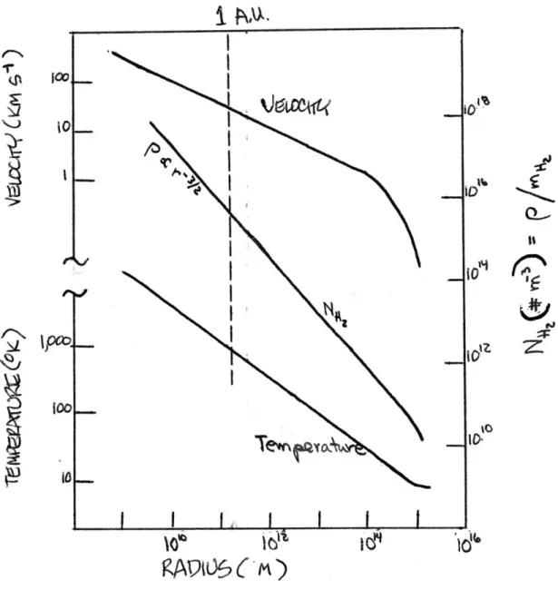
the "star" resembles a Hayashi pre-main sequence model (Hayashi, 1966). For a one-solar-mass protostar, the dependences of tem-perature and density on radius that Larson's models suggest are shown in Figure 2.1. Although his models are not applicable

to planetary formation, Larson concludes from the rapidity of the stellar formation process that planetary formation must occur simultaneously. This view, popular among some

theorists, adds complexity to investigations.

An approach that has proved fruitful inunderstanding planetary formation has been the examination of the chemical

equilibrium condensation sequence in a solar composition gas ( Gaustad, 1963; Lord, 1965; Larimer, 1967; Larimer and Anders, 1970; Lewis, 1972). Lewis' models (e.g. Lewis, 1974) show that the planetary densities and semi-major axes plot along an adiabat (or isobar) in a protoplanetary nebula (Figure 2.2). The remaining uncondensed

volatile nebula associated with the terrestrial planets would presumably have been dissipated somehow

as the sun began hydrogen fusion.

Safronov (1969) and Goldreich and Ward (1973) have at-tempted to follow the sequence of events beginning with con-densation and proceeding toward final planetary accretion. Starting with a rotating gas cloud, these investigators sug-gest the following sequence of events: During chemical

con-Pox

I

IOL.

I

I

I~

I

10z

RA9IU6, CM)

Figure 2 .1 Molecular density, temperature, and infall velocity in the en-velope of a one-solar-mass

protostar, following ~105 years of gravitational collapse starting fran an inial temperature of 10*K, radius of 1.6 x 10 m ~ 104 A.U., and densit

of 1.1 x 10-16 kg m-3 = mH x 3.3 x 101 H m-3.

2 H₂

Reproduced from Larson (1969a) .

Ioo

-- --

a

The abstract above and the following thesis are dedicated vessels water god, to the ancient Egyptian concept of Nu* $543

^NW

heaven

A member of the oldest company of the Egyptian gods, Nu was the deity associated with the primeval water, or heavenly Nile

(i.e. Milky Way). From the hieroglyphic inscriptions relating the Creation, we learn that the seeds of all life were believed

con-- sun god '

tained in the primordial Nu, whence Ra

and the earth were brought into existence.

*

Budge, E. A. W., 1904, The Gods of the Egyptians (1969 Edition, Dover, New York); see also Dreyer, J. L. E., 1906, A History

0 MgSiO3 %w1500~ _CaTiO D _{- MgSiO3} WFe-1000 FeS FeO e soo-erp ~ ce CC

-7

-6

-5

-4

-3

-2

-1

0

+1

log

PRESSURE (bcrs)

Figure 2.2 Chemical condensation temperature vs. pressure in a solar camposition proto-planetary nebula. Planetary formation temperatures

(as deduced fram present densities) and semimajor axes are plotted along an adiabat in a protoplanetary nebula (Lewis, 1974). Isobaric, rather than adiabatic, P-T profiles yield equivalent results for planetary densities (Lewis, 1974). Reproduced from Barshay and Lewis (1975).

densation, particles with typical linear dimension ~l0- m form and settle into a rotating disk, due to

gas drag. Goldreich and Ward then theorize a continuation in which gravitational instabilities in the particle disk form

-10 3-m-sized planetesmals in two accretional steps. The final step of this scenario (the accretion of planetesmals) remains to be investigated.

It is evident that knowledge of stellar and planetary forma-tion processes would be enhanced if the actual physical and dynamical conditions existing at some early point in

the formation process could be determined. Because the forma-tion of the young, metal-enriched Populaforma-tion I stars is

present-ly occurring along the arms of spiral galaxies, it is there that we shall now turn our attention.

CHAPTER 3

REGIONS ASSOCIATED WITH CURRENT STELLAR FORMATION

3.1 The Young Stars

The most readily apparent characteristics of stellar emis-sion are color (surface temperature or spectral class) and bright-ness (absolute magnitude)*. When the absolute magnitudes and

colors are plotted for gravitationally bound clusters of stars in our Galaxy, a Hertzsprung-Russell (H-R) diagram results, as shown in Figure 3.1 (Sandage, 1958).

*

The defining relationship for relative stellar magnitudes is B

m -m2 = -2.5 logi , where m designates apparent magnitude B₂'

and B the observed stellar brightness (received power per unit area). The brightness that would be observed at 10 parsecs de-fines the absolute magnitude M: M = m+5-5 log r, where

r = [parallax (arc sec)] is the stellar distance in parsecs. At the distance of the earth, the sun's observed brightness is

B ~ -1400 Wm-2 (the "solar constant"). Thus the solar luminosity, L (=4r 2B ), is ~ 3.9x1026 W. Were the sun at the standard

distance of 10 parsecs, it would yield the brightness

3.5 x 1010 WM-2. The stellar magnitude scale is calibrated such that this brightness would be produced by a star of ab-solute magnitude 4.8.

OB~

FG~~

0 0.4

Color

6-V)

Q,'. I,( 2.0

Figure 3.1 Hertzsprung-Russell (color-luminosity) diagrams for various galactic clusters and the globular cluster M 3. After Sandage (1958).

4

t4

_2V%2,

I.

I

I

I

I|

Pad

_es

6141

MA

M1 |oIi

_l|

A6E

I

r-S)

ic10'

21010i

In this figure, it is evident that the differentiating factor among such clusters is the point at which the high mass and luminosity blue stars begin to turn from the main sequence. Estimates of stellar lifetime on the main sequence are based on many factors, including luminosity, energy production in the

fusion conversion of hydrogen to helium, and the em-*

pirical mass-luminosity relationship . Such considerations lead to the calibration of Figure 3.1 in years. We note that the globular cluster M3, and the oldest galactic clusters (e.g., M67) would be assigned an age of ~5 x 109 years. An H-R diagram

for an elliptical galaxy would appear similar to that for a glo-bular cluster, thus implying a similar age. A younger galactic cluster, the Pleiades (see Figure 3.2), would have formed about 108 years ago, the approximate length of the Galactic rotational period (250 x 106 yrs); the youngest clusters shown in Figure 3.1 have an age of only-106 years and have been in existence a small fraction of one Galactic rotation period.

*

The luminosity of a star on the main sequence is related em-pirically to its mass by

L* _{21t p} = a( (

-E) 0

30

where2t designates stellar mass and X ~2.0xl0 kg. Thus

L* X*

log(-) _{= logI[a]+p log[ ~I'}

0 0

The constants a and p above are determined from

observations of main sequence binaries for which the semimajor axes and periods of each can be measured (Kepler's third law then al-lows 7, to be determined) .

Figure 3.2 The Pleiades, a galactic cluster ofo300 solar masses, radius ~3.5 pc., and age ~108 years. Lick Observatory photograph (Crossley reflector).

Consideration of the dynamical relaxation of clusters (Chandrasekhar, 1942; Wielen, 1971) indicates a relaxation time scale of -10 years for a cluster such as the Pleiades

(-300 solar masses, radius -3.5 parsec), and predicts correctly the observed radial velocity dispersion of 0.4 km s~1 (Titus,

1938) among its stars. Thus, as we progress to clusters younger than the Pleiades, we expect to encounter stars that have not yet relaxed dynamically, and therefore that have retained some effects

of the dynamics of their formation.

As we consider clusters younger than the Pleiades we also begin to reach 0-class stars bright enough

in the ultraviolet to ionize the gaseous remnants of their forma-tion. The younger a region, the more intense its ultraviolet radiation, and the more intact the remnant nebula.

3.2 H II Regions (Emission Nebulae)

These regions of interstellar ionization (primarily hy-drogen) are designated H I regions, as opposed to the neutral hydrogen HI regions. Also in the class of intragalactic emis-sion nebulae, but of different origin from the H11 emisemis-sion nebulae we are considering here, are the relatively infrequent planetary nebulae (Ring, Bubble, Dumbbell Nebulae) and the supernovae remnants (Veil, Crab Nebulae).

The photographic appearance of galactic spiral arm struc-ture is dominated by the presence of the bright H I regions

(see Figure 3.3). The spiral arms contain the young Population I stars, and the HI and H11 regions; in the nuclei, hydrogen is much depleted and the stars are old Population II

(characteris-tic of globular clusters and ellip(characteris-tical galaxies). Increasingly large and bright H11 regions characterize the progression of spiral galaxies from Sa* to Sc. In the progression from Sc to Sa, the arms become increasingly more tightly wound, and the mass of neutral hydrogen decreases (from -7% of the total mass to ~1% (Roberts, 1974)).

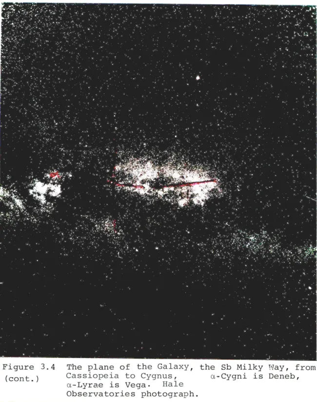
Our view of the Sb Milky Way (Figure 3.4) is similarly dominated by the H11 emission nebulae and associated dark HI clouds along the Sagittarius, Carina-Cygnus (Orion), and

Per-seus spiral arms. The constellations Cygnus, Lyra, and

Cas-siopeia are indicated for scale reference purposes in Figure 3.4. The North American Nebula (a typical H region of low emission measure) is conspicuous in Figure 3.4 near a-Cygni (Deneb).

The Andromeda Galaxy (M31), a member of our Local Group, is also visible in Figure 3.4. It has been only since 1924 that the scale of the universe has been sufficiently well established to distinguish the intragalactic distances (kiloparsecs) to

Galactic emission nebulae from intergalactic distances (mega-parsecs). The famous Curtis-Shapley disagreement (Curtis, 1919; Shapley, 1919) on the "island universe" controversy,

*

The classification system for galaxies was developed by Edwin Hubble (1926).

Figure 3.3 _{The Sc spiral galaxy M51 (NGC 5194) and its} satellite NGC 5195. Hale Observatories photograph (200").

Figure 3.4 _{The plane of our galaxy, the Sb Milky Way, from} Cassiopeia to Cygnus, a-Cygni is Deneb,

M 31 is Andromeda. Hale Observatories photograph.

Figure 3.4 The plane of the Galaxy, the Sb Milky Way, from (cont.) Cassiopeia to Cygnus, a-Cygni is Deneb,

a-Lyrae is Vega. Hale Observatories photograph.

culminating in a debate before the National Academy of Sciences on 26 April 1920, was finally resolved by Hubble's discovery of Cepheid variable stars in M31.

Continuing the progression of scale from Figure 3.4, we show the emission nebulosity associated with the "belt" and "sword" of the constellation Orion in Figure 3.5, where

regions displayed in subsequent figures are indicated. The star B -Orionis is Rigel, a (young) B7 star of -30 solar masses and absolute magnitude M = -7. In Figure 3.5, and in the sub-sequent Figures 3.6 and 3.7, the direct juxtaposition of low density H11 regions with dense HI clouds is evident. The

well known Horsehead Nebula (an obscuring HI region) is visible in Figures 3.6 and 3.7. The stars indicated in these figures correspond to those on the star chart, Figure 3.6b, prepared from the Smithsonian Astrophysical Observatory (SAO) Star Catalogue (1966). On the chart, a star's apparent brightness is proportional to the size of the marker.

We now proceed to examine characteristics of the Galac-tic H emission nebulae. The brightest optical emission lines emanating from the Galactic H_{1 1} regions are from H and for-bidden transitions of O1, 0111, and N11 (Bowen, 1928; Herz-berg, 1937). _{The two most intense lines originate from 0111}

0 0

transitions at green wavelengths of 5006.84 A and 4958.91 A. The relative intensities ofthe various nebular lines are in-dicative of the spectral class, and thus of the main sequence age, of

k-H

AL

4.

9*

- - *4

Figure 3.6 Nebulosity in the "belt" of the constellation Orion, near C- Orionis. Negative exposure

reproduced from the Palomar Sky Survey. I

+ _.7 + 13: 13 ₁₂₆₆ 311 f e_---3 + , ____

6EU_

57

?

(n

-Cz

A-Figure 3.6b Star chart corresponding to Figure 3.6 (Orion B). Star #105 is C-Orionis.

Figure 3. 7 The Horsehead Nebula (an obscuring H cloud) near C-Orionis. Yerkes Observatory photograph.

constituents (HI+HIT at -13.6 ev; O IO at ~35 ev; O ₁₁ m at ~55 ev) and the excitation which leads to the optical emission of the species is pro-vided by thermalized, several-electron-volt electrons. The optical emission thus acts to cool the H region. When there is insufficient ultra-violet for complete ionization, the appearance of a nebula is described as "radiation-bounded"; when there is insufficient

gas, the appearance of the completely ionized nebula is des-cribed as "gas-bounded". Reference to Figure 3.3 shows that bright H11 regions often have long (~102,3 parsec) gas-bounded

tails extending outward and backward (in a rotational sense) from the spiral arms.

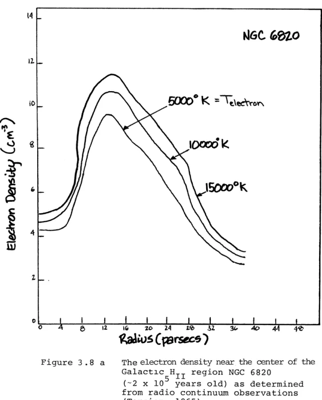
Younger than the Pleiades, emission nebulae such as NGC 6820 (optically obscured) are about 105 ,6 years old (Kahn

and Menon, 1961; Lasker, 1966). The central regions of such nebulae have been cleared due to the intense ultraviolet radiation of the

young stars, as evident from the electron densities displayed in Figure 3.8a. A well known example of this age class of H₁₁ regions is the Rosette Nebula (NGC 2237) in Monoceros.

The youngest H regions are -10 4 ,5 years old (Vandervoort, 1963; Lasker, 1966), and the nebulae are still relatively intact, as evidenced by the

electron density distribution of M16 shown in Figure 3.8b. Illustrative members of this youngest class of H11 regions are shown in Figures 3.9a (Orion Nebula, M42), 3.10a (Omega Nebula, M17), and 3.lla (IC 1795). Figures 3.9b, 3.10b, and 3.llb show

corres-Figure 3 .8 a The electron density near the center of the Galactic5 H region NGC 6820

(-2 x 10 years old) as determined from radio continuum observations

(Terzian, 1965).

Il*

i ro zo 24 ;Le I foalu-S

(Varsece )

Figure 3 .8 b The electron density near the center of the Galactic H region M 16

(~5 x 104 years old) as determined from radio continuum observations

(Terzian, 1965).

iso

Fo

Figure 3.9a The Orion Nebula (M 42, NGC 1976) in the "sword" of the constellation.

LI -V

16

Figure 3.9b Star chart corresponding to Figure 3.9a (Orion Nebula, M 42). Star #6 is the 06 class Trapezium star thought to be exciting the H region. The contour shown on this star chart, and tJse shown in Figures 3.10b and 3.11b, correspond to the outermost contour of the corresponding radio con-tinuum contour maps (Figures 3.9c, 3.10c, and 3.llc). +9

-So %5/

(0

-

+ 9

IT

16

Figure 3.10b Star chart corresponding to Figure 3.10a (M'17, Omega Nebula).

-44.

01'

-- #*

71'

Figure 3.lla IC 1795, a negative exposure reproduced from the Palomar Sky Survey.

OZ so'

(XZ

45

Figure 3.11 b Star chart corresponding to Figure 3 .la (IC 1795) . The regions of H 20 maser emission marked by _{squares and numbers are}

1] W3 (OH) and 2] W3C. U

4k s -0

ponding regions of sky from the SAO Star Catalogue (1966). As-sociated with these young optical emission nebulae are found radio continuum sources; the locations of these sources are

shown for photographs 3.9 a, 3.10a, and 3.lla in Figures 3.9c,

3.10c, and 3.llc, respectively. The locations of the radio continuum sources are at the heads of the extended gas-bounded tails, in close proximity to the H y-H interfaces.

-The radio-infrared spectrum of a typical continuum region is shown in Figure 3.12. The radio frequency portion of the spectrum in Figure 3.12 is indicative of thermal radiation from ionized hydrogen (e.g. Terzian, 1965). Observations of H I regions at the hydrogen recombination-line frequencies yield estimates of electron temperature and density, an rms value of internal turbulence, and a value for the radial velocity. Examples of such observations (Hoglund and Mezger, 1965; Mezger and Hoglund,

1967) are shown in Figure 3.13. The young H11 nebulae have electron tem-peratures of -10 0 *K, and estimates of mass deduced from their angular

ex-tent and density range from ~103 to ~105 stellar masses. Internal tur-bulence in these nebulae has an rms value of -20 km s . This value

compares with a Galactic rotation velocity for the sun of -300 km s , and an rms dispersion of ~15 km s among local group Population I stars. Use of the hydrogen recombination-line radial velocities with a model of Galactic rotation

(IAU 1963) yields kinematic distances (Becker and Fenkart 1963; Mezger and Hoglund, 1967). Figure 3.14 shows the re-sultant Galactic distribution of the radio H I regions in

15 - -05"20'-0--05"25 -- -CI) 70 6060 40 30 2) 100 35 --- _-05 h 3m 05 h 2m +---(1950) O0'- -M17 (G15.0-0.7) IC1795 -16*00' + G 133.8 +1.4 +62 00' - 0 0 5 L0 10 00 60 ~60 1 40 50'1 200 18m 8 17 m 40 Ca(1950) _23m 22m 02 2mm + - (1950)

Figures 3.9 c, 3.10 c, 3.11 c Radio continuum maps at 5 GHz of the H regions associated with a) the Orion Nebula (M 42), b) M 17 (Omega Nebula), c) IC 1795.

Contours are in units of antenna temparature

04

Figure 3.12 Radio-infrared spectrum of M 17 (omega Nebula). Reproduced from Johnston and Hobbs (1973).

Points denote observations; dashes indicate theory.

A theoretical derivation of the continuum radio flux

expected from a diffuse nebula is contained in Terzian (1965) .

e(OK)

A

3

2

eo & o k P->

Figure 3 .13 _{Hydrogen recombination line (n}

1 1 0 + nl_{0 9}; 5.009 GHz) observati-ons of M 42, M 17, and IC 1795. From Hoglund and Mezger (1965) and Mezger and H6glund (1967). Velocity shown is

with respect to the local standard of rest (LSR) .

,Ot40"A

4

N

v--;

Figure 3.14 Distribution of radio H I regions in the Galactic plane. Reproduced from Mezger and H6glund (1967). The local spiral arms are indicated. (Note that the current best estimate of Galactic distances places the sun about 15% closer to the Galactic center.)

which the local spiral arms are well defined.

Also evident in Figure 3.12 is the presence of an intense source in the infrared. This association with IR sources is representative of the regions of continuum radio emission

as-sociated with the young Galactic H11 regions. In the Orion Nebula (M42) the well known Becklin-Neugebauer infrared source was discovered in 1967; a succession of similar objects has been

detected more recently (Wynn-Williams, Becklin, and Neugebauer, 1972). Larson (1972) feels the characteristics of these ob-jects are indicative of ~5M protostars. Mapping observations indicate the point sources of infrared emission are interior to HI molecular clouds such as the Kleinmann-Low nebula in Orion. A wealth of molecules (over 26 to date) have been observed at

radio frequencies in the excited HI clouds associated with young Galactic H11 regions. Observations of these molecules lead to estimates of

11 -3

HI temperature and density. We adopt T~10*K and p-mH 2x1 H m as

repre-2 2

sentative (e.g., Snyder and Buhl, 1971; Thaddeus et al., 1971).

As a summary of our preceding examination of Galactic H I regions, we present in Figure 3.15 a schematic representation of a young Galactic H region with associated ionizing star and H cloud. In the region comprising the H I-H transition zone, the HI region is being compressed and heated. The H y-H

inter-face appears attractive as a primary stellar womb.

Remote investigation of the physical conditions existing in the H1 1-HI transition zones is facilitated by the presence of molecular masers emitting at radio frequencies. In Chapter 4 we consider these molecular masers further.

~-~cG~%Aeg~b

/7

I-Figure 3.15 Schematic representation of a young Galactic H region, its

ionizing 0 star, and associated H cloud.

W

CHAPTER 4

HIGH RESOLUTION RADIO OBSERVATIONS OF H 20 MASERS AS A MEANS OF PROBING REGIONS OF STELLAR FORMATION

4.1 Introduction

We wish to examine those regions in our Galaxy associated with current stellar production at a

sufficiently high resolution to enable

physi-cal conditions and dynamics associated with stellar formation to be deduced. To succeed in such an endeavor two primary

re-quirements must be satisfied: (1) the technological ability to examine appropriate regions, at typical distances of ~103 parsecs, with sufficient angular resolution to discern spatial scales

of ~l A.U at the radio sources (since 1 A.U. at 1 parsec is equivalent to 1 arc second, the required angular resolution is 10-3 arc second) ; and (2) the presence of suitable

microwave sources.

The technique of very long baseline radio interferometry (VLBI) is capable of providing the specified angular resolu-tion. By combining simultaneous observations recorded at

widely separated radio telescopes, VLBI provides angular reso-lution approximately equivalent to that of a single radio

telescope with diameter equal to the separation between obser-vatories (the length of the "baseline"). A brief mathematical

introduction to VLBI follows in Section 4.2.

The potential ability of the known molecular masers (OH,, H₂0, Sio) to provide suitable radio sources for our purposes is

selection of H₂0 masers for further detailed examination in this investiga-tion is justified. The thrust of this investigainvestiga-tion is directed toward ex-tracting the existent dynamics and physical conditions in the regions of in-terest from radio observations of H20 masers. In the final section of this chapter (Section 4.4), we begin _{this endeavor by describing the H20 6 16+523} maser transition in greater detail.

4.2 Very Long Baseline Radio Interferometry

In very long baseline interferometry (VLBI) the emission of a radio source in a frequency band referenced to the local standard of rest is simultaneously recorded at two radio ob-servatories. If X ₁ (t) is the signal in this frequency band that is arriving at the first telescope from an infinitely dis-tant source at time t, then the corresponding signal arriving at the second telescope is X2 (t + T) = X₁ (t). If atmospheric and ionospheric effects are neglected, the delay, T, equals B e s/c, where B is the baseline vector from telescope 2 at time t + T to telescope 1 at time t, s is the unit vector in the direction of the source, and c is the speed of light. The delay may equivalently be expressed in terms of a phase as $ = 27vT, where v is the microwave observing frequency, and undergoes a sinusoidal variation due to the sidereal rotation of the earth.

The variation of the delay with s provides the angular resolution of the interferometer. If the baseline vector is projected onto the plane perpendicular to s (the

"celes-tial sphere") in the direction of s, it will describe a diurnal ellipse. At any given time, the delay will be constant along lines on the celestial sphere that are perpendicular to the projected baseline. The use of additional observatories and the rotation of the earth permit many independent determina-tions of delay over a sidereal day. In this manner information may be compiled about the angular distribution of radio emission

in right ascension (a) and declination (6). When the radio source is composed of unresolved point components, compilation of a data set which yields unique determinations of position is relatively straightforward, as will be demonstrated in Sec-tion 5.1.1.

4.3 Molecular Maser Radio Sources

The first astrophysical molecular maser source detected was OH (X = 18 cm; v9= 1.6 GHz) in 1965 (Weaver, Williams,

Dieter, and Lum, 1965), followed by H₂0 (A= 1.35 cm; v = 22 GHz) in 1968 (Cheung et al., 1969), and by SiO (X = 0.34 cm; v₀ = 86 GHz) in 1973 (Snyder and Buhl, 1974). Astrophysical conditions required to produce these molecular masers are apparently so selective that the sources of the maser radio emission require the angular accuracy provided by VLBI to resolve. Although the physical extent of the "masing" regions is small, the maser am-plification mechanism provides sufficient photon output to allow their detection on earth. The small size of these regions first began to be appreciated when the initial radio astronomical

ob-servations utilizing interferometry determined that the radia-tion from OH sources originated from as yet unresolved, spatially

separate, Doppler shifted emission features (Moran, 1968). Since their initial discoveries, numerous Galactic* OH, H 20 and SiO masers have been located. OH, H20, and SiO masers

have been found associated with infrared stars, while OH (Type I) and intense H20 masers are found associated with H11 regions. The high dissociation energy of SiO permits the mole-cule to remain intact at the higher thermal temperatures in the infrared star environment which are responsible for population of the first and second vibrational states from which the ro-tational maser transitions originate. A more complete

dis-cussion of the SiO maser transitions is contained in Snyder and Buhl (1975). As yet no VLBI observations of SiO have been successful.

For the purposes of this investigation we will consider further only the intense OH and H20 masers associated with

Galactic H11 regions. The Doppler shifts of OH and H20 masers

are found to fall well within the turbulence broadened con-tinuum envelopes of the associated H regions (see Figure 3.13). The radial velocities of the OH and H20 sources often overlap but no

correla-tion is apparent. As the technological state of the radio in-terferometer observations improved, it has been possible to

*

An unsuccessful attempt to detect H 0 masers in M31 (Andromeda) was made by the author at Haystack Observatory. In the

ob-serving program, designated Reisz-1, -25 bright H regions iden-tified by Baade and Arp (1964) were searched.

determine accurately the relative angular distribution of emission features, and their apparent transverse extents. OH and H 20 masers are found to be distributed over regions which are spatially co-incident to within the absolute accuracy of the separate observations (a few arc seconds). Typical OH emission features appear to be

~10 2 A. U . in transverse extent, while those H20 features resolved are

-26 -2 -1 typically ~1 A.U. The maximum observed radio flux density (10 -2 n Hz

= Jy) from H20 masers is often an order of magnitude larger than that observed from the associated OH sources.

The OH spectra result from A doubled transitions in the 2

23/2' J=3/2 rotational state. A doubling arises due to the interaction between the unpaired electron and the molecular rotation in which two electronic configurations are possible --a higher energy orient--ation in which the electron distribution

is along the molecular rotation axis, and a lower state in which it is in the plane of rotation. Each A doublet is

fur-ther hyperfine split into two (21+1; I = 1/2) F levels, where

F = J+I, due to the interaction between the nuclear magnetic moment of the hydrogen and the molecular magnetic moment

(resulting, primarily, from the unpaired electron). In Type I OH sources the AF=0 A doublet transitions at 1665 MHz and

1667 MHz are observed to be the most intense.

In a manner similar to the case of OH, the H20 J=5,6 molecular rotational levels are each hyperfine split into three

hyper-fine frequency splitting in the case of H20, however, is

ap-proximately a factor of Pnuc melectron - 1 less than in the 1_{Bohr proton 1836}

case of OH, where y denotes magnetic moment. Thus the frequency separation of hyperfine components in the H 20 maser transition will be~ (1720-1665) MHz

1836

- 30 KHz, and the susceptibility of H20 molecules to the presence of weak magnetic fields (-5 x lo-3gauss; Beichman and Chaisson, 1975)

in the sources would be about 1836 less severe than for OH. Calculations of molecular abundances based upon chemical equilibrium in a solar composition gas are shown in Figures 4.1, 4.2, and 4.3 for a range of temperature and density relevant to a protoplanetary nebula*. It is evident from these figures that in the low temperature, high pressure regime (below the T-P contour of the H-H2 boundary indicated in the figures) in which molecules primarily exist, the H20 molecule is the most abundant of the masing molecules.

In several ways thus far we have found that the H20 mole-cule offers us the best potential probe of those regions along the spiral arms of the Milky Way associated with current

stel-lar formation. There remains little further impediment to an observational continuation to this investigation since ad-ditionally: (1) low noise receivers and spectral correlators

exist at Ku band; (2) the earth's atmosphere and ionosphere

at Ku-band do not corrupt, radio interferometric observations significantly, even on the longest of earth-based baselines (Burke et al.,

*

The computations from which these figures were prepared were provided by S. Barshay and J. S. Lewis, Department of Earth and Planetary Sciences, M.I.T.

2i

100

0:#

I-j

.

-

-12.

-11

-10

-

..

7

-m

\o

%

PRESSkREars

Figure 4 .1 T-P contours of C (H₂0) -the ratio of the H20 partial-pressure to the total pressure for solar composition gas in chemical equilibrium. Above the H-H₂ T-P boundary marked, H is more prevalent than H

Over the T-P range shown here, C (H20) ~ C (CO) . The computa ions from which this figure, and Figures 4.2, and 4.3 were prepared

were provided by S. Barshay and J. S. Lewis, Dept. of Earth and Planetary Sciences, M.I.T.

-' -12. -I -10

-i

PRe

S$AE

.-'

(64rs)

Figure 4.2 As in Figure 4.1, but for SiO instead of H20. I.00

190o

ws

.19

'OOO

%(Soo

\D

cc

low

.

o

Pr

(br

Figure 4.3 As in Figure 4.1, but for OH instead of H₂0.

1972); and (3) the H20 transition has been well studied in the

laboratory (Bluyssen, Dymanus, and Verhoeven, 1967; Kukolich, 1969). Before beginning the description of the experimental observing program in Chapter 5, we will first review the H20 ro-tational transition in more detail in the following Section. 4.4 The H20 616 _ 523 Maser Transition*

Due to the interaction between J and the total nuclear angular-momentum I (for the two hydrogens I = 1 +

1

laboratory (Kukolich, 1969) is summarized in Table 4.1 and illustrated in Figure 4.4. The spectrum of the spontaneous emission from the transition calculated for conditions of

local thermodynamic equilibrium (LTE) for a distant

In the spectroscopic notation JK1K designating an asymmetric top rotational level, K1 and K2 are the projections of J, the total molecular angular momentum, along a symmetry axis of the molecule for the cases of the limiting prolate and the limiting oblate symmetric tops.

Table 4.1

Hyperfine Components of the 616 + 523 H20 Rotational Transition v* (kHz) - 35.86± .05 - 2.79± .05 40.51± .05 173.2 ±2 217.9 ±2 Relative Intensityt .385 .324 .273 .009 .009 + 6 394 .00006

Frequency relative to 22.23507985 GHz (frequency of the intensity-weighted mean)

tIn _{local thermodynamic equilibrium (LTE) ; values from} Townes and Schawlow, 1955.

Values for the AF = +1 transition from Sullivan (1971). F 7 +6 6 + 5 5 4 6 +*6 5 +5

:

4

5

IN THE

616

_{- 523}

LINE OF H

0

133

100

200

RELATIVE FREQUENCY (KHz)

Figure 4. 4 The hyperfine components of the 616 -* 523 rotational

transition of H20. Data from Kukolich (1969).

A

z

-w

301-201

it

(5

43

101-

33-300

(5-+-6)

400

cloud of H20 gas at various kinetic temperatures (10, 100,

1000*K) is shown in Figure 4.5. For each hyperfine component

j,

2 mH20 vz f. (vz) = a exp [ 2

j 2kT

V v

The first order Doppler shift v-va Av = - z may be introduced to determine the corresponding frequency distribution

(Av) 2 f.() a. exp[-2a2 J where kT mH 0 H20

and where v is an observed frequency, v0 is the mean of the hyperfine

fre-quencies, and X E c/vo. The full width

at half power (fwhp) of f. equals 2.3548 a.. The

J J

spectrum for the transition is obtained here by superposing the individual spectra of the three hyperfine lines for which AF=-l. Computational de-tails are contained in Appendix B.

Because the energy spacings between the hyperfine levels in H20 are so small with respect to the energies of the relevant molecular rotational levels, the assumption of an LTE population distribution appears valid for almost any

excitation mechanism. None of the pumping mechanisms yet proposed for the H₂0 maser [infrared (Litvak, 1973); ultraviolet (Oka, 1973); collisional

(de Jong, 1974)] are capable of selective population of hyperfine levels. This is unlike the case of OH (e.g., Gwinn et al., 1975).

Figure 4.5 The spectral appearance of the spontaneous emission from the H₂0 616 + 523 rotational transition computed for kinetic

temperatures of 100, 100*, and 1000*K. 0=22.2350 7 9 8 5 GHz. A radial

Velocity of 1 km s-l corresponds to a frequency shift of -74.1 kHz.

,4t

zoo 100 - ZOO

(K4t)-CHAPTER 5

RADIO OBSERVATIONS OF H 0 MASERS

5.1 VLBI Observations and Analysis

The high signal-to-noise ratio that can be obtained in ob-servations of H20 maser sources may be exploited to make extremely accurate determinations of the relative angular positions of emis-sion features in a given source, and to examine the emisemis-sion spec-tra of individual features at high specspec-tral resolution. Measure-ments of relative angular positions over time will yield the

relative transverse velocities of neighboring maser regions. Analysis of the spectra of individual emission features yields information about the physical conditions as well as the radial velocities characteristic of these regions.

With these goals in mind we selectively analyzed some of the VLBI observations made in 1970 June, 1971 February, and 1971 March, with antennas at the following radio observatories: Haystack

Observatory, Tyngsboro, Massachusetts; Naval Research Laboratory, Maryland Point, Maryland; and National Radio Astronomy Observa-tory, Green Bank, West Virginia and Tucson, Arizona (Johnston

et al., 1971; Moran et al., 1973; and Reisz et al., 1973). In these observations the incoming signal* at each observatory was mixed with the outputs of stable frequency sources (local

oscil-lators) and the resulting video signal was clipped, sampled, and digitally recorded on magnetic tape, using the Mark I recording system (Bare et al., 1967).

*

All observations were conducted with horizontal (E) linear polarization, referenced to Haystack Observatory.

Each VLBI observation consisted of ~150 seconds of data re-corded "on source", followed by ~30 seconds of "off source" calibration data. The local oscillators were set such that the total output frequency equalled the minimum frequency in the desired band, v in , plus the a priori Doppler shift

d, Vmin introduced by the sidereal rotation and orbital revolu-tion of the earth at the start time of an observarevolu-tion. In the processing of each tape-pair, the bit strings from two observa-tories were aligned (geometric delay removed) and

cross-cor-related; the cross-correlation was then corrected for clipping (Van Vleck and Middleton, 1966), Hanning weighted, and Fourier transformed to yield the complex cross-spectrum in discrete form (e.g. Moran, 1976):

M L

S[v + (k-1) Av] = Z sin { E X₁ [ (,-l) At] (5.1)

mi m=l 2

X₂[ (k-l) At + (m-l) At] }H [(m-l) At] exp[2 Ti (m-l) At(k-l) Av]

where X and X2 are the clipped, sampled, and aligned forms of the video signals from two observatories; At=(7.2 x 105 l s is set by the Mark I system; 2AV = 2(MAt)~1 = spectral

resolu-1 -l

tion; H[(m-l)At] = 1 [1 + cos(m-l) 7M ] is the Hanning weighting 23

function; L = number of bits in each processed sample = 1.44x 10 3 M = number of delays in cross-correlation = number of spectral channels in transform; and k, Z, and m are the respective

processing of the cross-spectra over the duration of each ob-servation (~150 s), the fringe phase corresponding to the fre-quency channel that contained the spectral maximum of the most intense feature was used as a reference for fringe-phase rota-tion.

5.1.1 Accurate Relative Positions of H20 Emission Features

To determine accurately the angular position of a particular feature with respect to the reference feature, we must determine both the relative fringe rate and the relative phase for each observation. For these purposes, M in Equation (5.1) was chosen as 36, providing a spectral resolution of about 40 kHz. To determine the fringe rate with respect to that of the reference

(first time derivative of the relative fringe phase), the cross-spectra were integrated over the duration of each observation with the relative phase corresponding to each spectral channel counter rotated by (t-t. .)A$ where t.. is the start time of the

ij trial

th th

j observation on the i baseline and A trial is a trial value for the relative fringe rate. The value of A~trial that yielded the maximum fringe amplitude for the feature of interest upon integration was chosen as the relative fringe rate,

A$(t. .). The relative phase, A$(t. .), of the feature referred to t . .,was then taken to be the arithmetic mean of the relative phases

deter-mined about oce each second over the observation, each counterrotated by the appropriate (t-t .. ) A$ (t ..). Such estimates of relative phase are ambiguous in the sense that they represent the relative phase modulo 2'rn radians (n being some integer). Estimates of relative fringe rates alone, however, may be combined to yield unique maps of the relative positions of emission features (Moran, 1968; Moran et al.,

1973). An example of such a map for H 20 masers in W3(OH), associated with the optical H1 1 nebula IC 1795, is shown in Figure 5.1. The source W3 (OH) was selected for our purposes here because all five features were within about 2 arcseconds, and also within the 360 kHz observing bandwidth.

By statistically combining estimates of relative fringe rates and relative fringe phases, unambiguous determinations of relative positions can be made which are about two orders of magnitude more accurate than estimates that may be obtained from the relative fringe rates alone. A method devised for obtain-ing accurate estimates of relative position may be described as follows (Reisz et al., 1973):

We consider the angular separation of a particular spectral feature at fre uencl v frcm a reference feature at frequency v in the relative coordinates Aa in

right ascension and A6S in declination. Assuming the errors in the relative fringe rates to be independent random variables distributed in a Gaussian manner, we obtain, from these data alone, the joint probability density for the separation:

p(Aa,A6) = 1/ex 1 -1 (5.2)

0 ~27r jyP 112

where the row vector X has the two components Aa-Aa*, A6-A6*;

ipI

es-Iu~

-51.2

-47.5-

Aa(I cos 6 (ARCSECONDS)

Figure 5.1 Radio interferometer map of H₂0 emission features associated

with the optical nebula IC 1795. Masers are labeled by their radial ve,

locity (kIm/sec) . kII and b1I _{are Galactic longitude and latitude (LAU 1958).}

Reproduced from 1hbcan et al. (1973).

01-

-48.8

49.7

-0.5

-1.0

-1.5

,+ -50.4

timates Aa* and A6*.

The estimates of the relative fringe phases are ambiguous in the sense that they represent the relative phases, modulo 27n radians (n some integer). An instantaneous determina-tion of relative fringe phase for a particular baseline and

source may be represented as

A$(t) = c(Aa,A6;t) + e + 27Tn (5.3) in the strong signal case, where e.(<<2r) is the error in the

(ambiguous) phase determination, and the functional form of 0 is given by

O(AaA6;t) ~- 2 v[B(t)-i(a +Aa,6 +A6) - B(t) -( , )]

c o o o o

(5.4) where aof, 6 0 are the coordinates of the reference feature. These coordinates and B are generally known well enough to allow us to neglect their uncertainties when estimating

rela-tive angular positions. Since clock-synchronization errors and the effects of the propagation medium on the relative fringe phase cancel almost completely, they contribute neg-ligibly to e, leaving (thermal) receiver noise as the primary source of error and justifying our modeling of 6 as additive Gaussian noise.

If we consider that Equation (5.2) provides the joint a priori probability density of Aa and A6 and that all values of the integer n in Equation (5.3) are equally probable, we may write the conditional probability density for Aa and A6,

given the set of independent relative fringe-phase estimates A$(t. .), as

1J

p(Aa, A6|A ) c p (Aa,A6) x 1 H exp{A$ (t) i=1 j=1 n=-oi

2 2

- 2fn - 4(Aa,A6;t. .)] /2a. } (5.5) where a is the standard deviation of the relative fringe phase from the

jth

We take as our final estimate of the relative angular position of the feature the value of (Aa,A6) for which the

conditional probability is a maximum. This estimate of

relative position can be found quickly for "reasonable" data sets by systematic evaluation of p over successively finer two-dimensional grids in the (Aa,A6)-plane. Because of the slow variation of p0 with a change in either Aa or A6,

com-pared to the corresponding change in the other factors in p, the presence of p₀ serves primarily to delimit the area of search for the maximum of p. By the same token, the estimate determined by the above algorithm will not differ significantly from the maximum-likelihood estimate of the relative position.

The information content of the interferometer observations is illustrated in Figure 5.2 for the location of the -47.5 km s~1 feature shown in Figure 5.1, relative to the -48.8 km s reference feature.

-0.20- 18:30 UT -0 FRINGE -PHASE POSITION U) FRINGE -RATE POSIT ION -0.252 -1.85 - 1.90 - 1.95

cos8c0 Aa (ARC SECONDS)

-0.20- 19:30 UT

--U) 0

z

F E -FR INGE -PHASE

WFRINGE -RATE PSTO

POSITION

-0.25- 1--2'

3-2

-1.85 -1.90 -1.95

cos 8o Aa (ARC SECONDS)

Figure 5.2 Lines of constant relative frinye phase Al(t-j)2'rn for the -47.5 km s- feature relative to the -48.8 km s-1 reference feature for the Haystack-NRAO (1+ 2) and the NRL-NRAO (3-+ 2) baselines at 18:30 and 19:30 UT on 1971 March 28. Lines are shown for each baseline for three consecutive values of n (see text) in the vicinity of the feature position determined from analysis of relative fringe-phase and fringe-rate data. Also shown is the feature position determined from analysis of relative fringe-rate data alone.

Combination of the information from eleven* observations of W3(OH) on three interferometer baselines (Table 5.1) yields the relative positions presented in Table 5.2. Figure 5.3 illustrates the accuracy of these determinations by displaying the contours of constant probability density for the relative location of the -47.5 km s~ feature.

Observations using cryogenic (low system temperature) receivers on the longest earth-based interferometer baselines should allow the accuracy of such determinations to be improved to 10-5 arc second, sufficient to determine within one year transverse velocities of 1 km s~1 between features at the 2.5 kpc distance of W3 (OH). 5.1.2 Spectra of Individual H20 Emission Features

Selected interferometer observations were also processed to examine the spectra of individual H20 emission features. For this purpose, M in

Equa-tion (5.1) was chosen as 360, equivalent to a frequency resoluEqua-tion of about 4 kHz, and the most intense features were examined. This value of M, and hence the frequency resolution, was selected to ensure that individual H20 hyperfine

components would be fully resolved. Because features that are spatially re-moved from the feature of interest appear at different fringe rates, integration of the cross-spectra over an observation allows the effects of these spatially distinct features to be removed. The spatial discrimination provided

by interferometric observations is an important advantage of such observations over those conducted using a single radio

*

Eight of the eleven observations are statistically independent. The information gained from the required phase closure on three base-lines simultaneously is equivalent to that from the observation on the third baseline, but contains statistically dependent noise.