HAL Id: hal-00318407
https://hal.archives-ouvertes.fr/hal-00318407
Submitted on 29 Nov 2007
HAL is a multi-disciplinary open access
archive for the deposit and dissemination of
sci-entific research documents, whether they are
pub-lished or not. The documents may come from
teaching and research institutions in France or
abroad, or from public or private research centers.
L’archive ouverte pluridisciplinaire HAL, est
destinée au dépôt et à la diffusion de documents
scientifiques de niveau recherche, publiés ou non,
émanant des établissements d’enseignement et de
recherche français ou étrangers, des laboratoires
publics ou privés.
a piecewise PV inversion technique
L. Fita, R. Romero, C. Ramis
To cite this version:
L. Fita, R. Romero, C. Ramis. Objective quantification of perturbations produced with a piecewise PV
inversion technique. Annales Geophysicae, European Geosciences Union, 2007, 25 (11), pp.2335-2349.
�hal-00318407�
www.ann-geophys.net/25/2335/2007/ © European Geosciences Union 2007
Annales
Geophysicae
Objective quantification of perturbations produced with a piecewise
PV inversion technique
L. Fita, R. Romero, and C. Ramis
Grup de Meteorologia, Departament de F´ısica, Universitat de les Illes Balears, Ciutat de Mallorca, Spain
Received: 14 May 2007 – Revised: 21 September 2007 – Accepted: 23 October 2007 – Published: 29 November 2007
Abstract. PV inversion techniques have been widely used
in numerical studies of severe weather cases. These tech-niques can be applied as a way to study the sensitivity of the responsible meteorological system to changes in the initial conditions of the simulations. Dynamical effects of a collec-tion of atmospheric features involved in the evolucollec-tion of the system can be isolated. However, aspects, such as the def-inition of the atmospheric features or the amount of change in the initial conditions, are largely case-dependent and/or subjectively defined. An objective way to calculate the mod-ification of the initial fields is proposed to alleviate this prob-lem. The perturbations are quantified as the mean absolute variations of the total energy between the original and mod-ified fields, and an unique energy variation value is fixed for all the perturbations derived from different PV anomalies. Thus, PV features of different dimensions and characteristics introduce the same net modification of the initial conditions from an energetic point of view. The devised quantification method is applied to study the high impact weather case of 9–11 November 2001 in the Western Mediterranean basin, when a deep and strong cyclone was formed. On the Balearic Islands 4 people died, and sustained winds of 30 ms−1 and precipitation higher than 200 mm/24 h were recorded. More-over, 700 people died in Algiers during the first phase of the event. The sensitivities to perturbations in the initial condi-tions of a deep upper level trough, the anticyclonic system related to the North Atlantic high and the surface thermal anomaly related to the baroclinicity of the environment are determined. Results reveal a high influence of the upper level trough and the surface thermal anomaly and a minor role of the North Atlantic high during the genesis of the cyclone.
Keywords. Meteorology and atmospheric dynamics (Mesoscale meteorology; Middle atmosphere dynamics)
Correspondence to: L. Fita
1 Introduction
Potential Vorticity (PV) as a conservative quantity for adia-batic and frictionless conditions has been revealed as a good variable to study the structure and evolution of cyclones (Hoskins et al., 1985; Gyakum, 1983b; Huo et al., 1995; Hakim et al., 1996). The piecewise PV inversion technique (Davis and Emanuel, 1991) can be used as a way to modify the initial conditions of numerical simulations. The sensitiv-ity to changes in the initial conditions has been used in sev-eral dynamical studies of intense storms (Huo et al., 1999a,b; Romero, 2001a; Homar et al., 2002, 2003). This approach has been shown as a powerful tool towards the understanding of important atmospheric aspects related to the cyclogenesis, such as baroclinic and barotropic development and convec-tion. Piecewise PV inversion allows one to study the impact of the selected PV anomalies on the structure of the initial at-mospheric fields and on the subsequent dynamical evolution of the simulated circulation systems.
However, the method of designing perturbed simulations via PV inversion exhibits some particular aspects that are case-dependent, and presents some subjective choices that can deeply influence the results. Some of them are: iden-tification of the PV features, magnitude of the modification of the initial conditions, a set of balance equations used in the inversion, and boundary conditions for the inversion. In this study, the piecewise PV inversion technique of Davis and Emanuel (1991) is used. In order to diminish the subjectiv-ity of the procedure, an objective way to quantify the initial modification introduced in the perturbed simulations is pro-posed. The quantification of the perturbation is expressed as the mean absolute variation of the total energy between the initial and the modified fields, considering the whole hori-zontal domain of simulation and all vertical levels. The capa-bility to compute the “total amount” of the introduced mod-ification makes an objective control of one important aspect of the PV inversion technique possible, favouring meaningful intercomparisons of perturbed scenarios.
Fig. 1. Sea level pressure (every 4 hPa, solid line), Potential temperature at 850 hPa (every 4 K, dashed line) and Isentropic Ertel PV at
330 K (1 PVU=10−6m2Ks−1kg−1, coloured field) from ECMWF analyses on 10 November 2001 at 00:00 UTC (top left), 10 November at 12:00 UTC (top right), 11 November at 00:00 UTC (bottom left) and 11 November at 12:00 UTC (bottom right).
The 9-12 November 2001 cyclone has been described by the authors as one of the most intense events in the West-ern Mediterranean basin during the last 25 years. The case is a deep episode of a three-dimensional cyclone classifica-tion done by Campins et al. (2006). It has been also widely studied (Davolio and Buzzi, 2004; Tripoli et al., 2005; Ar-gence et al., 2006). In 24 h a strong and deep vortex was formed. As a result, heavy precipitation and strong winds were recorded in Algiers and in the Balearic Islands. Seven hundred people died as a result of severe floods in Algiers, and 4 people died in the Balearic Islands, where sustained winds of 30 ms−1and precipitation above 200 mm/24 h were recorded and about two million trees fell down on the Mal-lorca Island.
The work is structured as follows: the second section de-scribes the cyclone event, followed by a discussion and for-mulation of the energy-quantification method of the initial perturbed conditions (Sect. 3). A fourth section with the re-sults of the November 2001 storm is presented, and a final section of conclusions is also given.
2 Case description
The case is a clear and strong example of a Pettersen-Smeybe class B cyclone evolution (Pettersen and Smebye, 1971), in which a cyclone is formed in a pre-existing upper level trough environment. The genesis and evolution of the case presents similar characteristics to the case that occurred in December 1979 in the Western Mediterranean basin (Homar
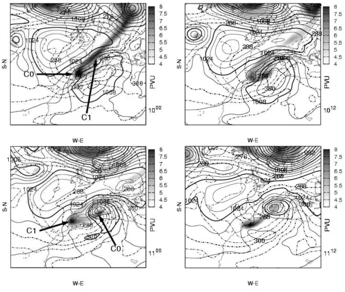
et al., 2002). On 10 November 2001, a disturbance was formed at the surface to the south of the Atlas mountains range (see Fig. 1, with the ECMWF analyses maps). A sig-nificant upper level disturbance was located over central Eu-rope, extending from the Iberian peninsula to the Baltic Sea. This upper level disturbance shows a structure of two high PV positive anomalies (C0, C1, see labels in Fig. 1). Over the Mediterranean Sea there was a post storm situation with residual convective activity (not shown). As a result of the surface African low and the upper level disturbance, strong thermal gradients developed over the western Mediterranean basin. The low level cyclone moved northwards; meanwhile, the upper level disturbance translated southwards. While the low-level low crossed the Atlas mountains, the upper level PV positive centres described a singular relative rotational movement, attributed to their interactions through PV advec-tion. Mutual interaction between different positive PV vor-tices has been shown as an important factor that contributes to the cyclogenesis (Hakim et al., 1996). Although in this case, there was not a merging of the PV centres.
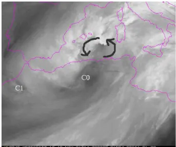
On 10 November, at 18:00 UTC, a strong interaction be-tween upper level and low level disturbances was established. This is identified in Fig. 2 as the closeness between the up-per level disturbance (see the tropopause fold, or free cloud area), and a strong cyclonic cloud structure (cyclone, indi-cated by curved arrows). These configurations of proxim-ity between strong surface thermal gradients and upper level trough disturbances become the ideal environmental condi-tions, under an appropriate vertical wind shear, to produce the baroclinic growth of disturbances. It has been described as one of the most important baroclinic processes from which deep cyclones can be formed (Hoskins et al., 1985; Bleck, 1990). From that time the cyclone crossed the Algerian coast and reached its mature state (11 November at 00:00 UTC), while strong cloud formation was present in the area. Strong winds were produced at the surface (33 ms−1sustained wind records were registered on the Balearic Islands between 11 November 00:00 UTC and 06:00 UTC). Some time later the upper-low level interaction weakened because of the south-ward movement of the upper level disturbance and the north-ward motion of the cyclone. At this point the cyclone weak-ened and could be described as an eastward movement while it approached the Sardinia Island.
The case will be studied using the MM5 nonhydrostatic primitive equation mesoscale model (Grell et al., 1994). A control simulation is run with one domain, with a horizon-tal resolution of 54 km and 23 vertical levels. The simulated period comprises the interval between 10 November 2001 at 00:00 UTC and 12 November 2001 at 00:00 UTC. Control simulation will prescribe the main characteristics of the cy-clone that will be compared to the simulated cycy-clones ob-tained from the PV-based sensitivity tests. All MM5 sim-ulations will be run in the same configuration based on a graupel(reisner2) scheme for the explicit moisture processes, a Kain-Fritsch scheme for the cumulus convection, a MRF
Fig. 2. Normalised Water Vapour METEOSAT7 image on 10 November 2001 at 22:00 UTC. EUMETSAT source.
parametrisation for the planetary boundary layer and the “rrtm” scheme (long wave) for the atmospheric radiation.
In order to track the baroclinic mechanism, the trajecto-ries of “C0” (the southwestern upper level PV vortex inside the upper level trough on 10 November at 00:00 UTC, Fig. 1 of ECMWF analyses) and the surface cyclone are analysed. During the initial phase of the evolution, control simulation results show that meanwhile, the upper level positive vortex C0 has moved southward, the cyclone has moved northward. In this way the low-level disturbance and C0 became closer (10 November at 12:00 UTC in Fig. 3). While the relative horizontal distance between the upper and low -level distur-bances decreased, the cyclone and C0 increased their inten-sity as a reflection of the baroclinic theory of phase coupling between the upper and low level disturbances (Hoskins et al., 1985). However, the cyclone reached its mature state on a negative baroclinic-phase (C0 is located east relative to the cyclone, Fig. 3 on 11 November at 00:00 UTC).
In this phase of the cyclone evolution, the cyclone reached the Mediterranean coast. Latent Heat Flux from the sea sur-face and the vigorous release of latent heat due to a strong cloud formation at mid levels (see water vapour satellite im-age in Fig. 2) could contribute to the intensification of the cy-clone. An intensification of cyclones, due to the diabatic ef-fects induced by the sea, has been detected in other cases, like in the North Atlantic “bombs” (Sanders and Gyakum, 1980; Kuo et al., 1991a,b), or other Mediterranean cases (Homar et al., 2002; Romero, 2001a). Moreover, the block-phase mu-tual interaction of the baroclinic process is also shown by the increasing central value of the C0 (Fig. 4). A significantly different behaviour between the two upper level vortices is observed in the same figure; whereas C0 became deeper, the other centre (C1) remained constant during the mutual
Fig. 3. Control simulation results. Left panel: Evolution of the position of the cyclone (dashed line) and the C0 (slash-dot line), date of
position is included ([DD][HH]). Right panel: Evolution of the central pressure of the cyclone (hPa, y-axis left) and its relative horizontal distance with C0 (km, y-axis right) since 10 November at 12:00 UTC. Relative horizontal distance is the distance between the positions of the centre of C0 and the cyclone. Positive(Negative) values of the relative distance occur when the cyclone is located eastward (westward) from C0.
Fig. 4. Simulated central value (PVU) of the two upper level
vor-tices C0 and C1, that are embedded within the upper level trough.
interaction period (10 November 15:00 UTC to 11 Novem-ber 00:00 UTC; see Fig. 4). It is shown how C0 preserves
its PV during the African phase of the cyclone. However, when the cyclone reached the sea, strong diabatic processes developed and C0 suffered an important increasing of its PV value. Meanwhile, C1 conserves its PV during almost the entire period of simulation.
During the African phase of the cyclone evolution (from 10 November 00:00 UTC to 10 November 18:00 UTC), the cyclone shows low vorticity (see Fig. 5). When the cy-clone reached the sea it attained the mature state (11 Novem-ber 00:00 UTC), depicted as: lowest surface central pressure value (988 hPa) and strong geostrophic vorticity (more than 30×10−5s−1 at the centre of the cyclone, computed using 200 km resolution geopotential data as in Campins et al., 2000).
3 Objective quantification of perturbations
The piecewise PV Inversion technique explained in Davis and Emanuel (1991) is used in the study. It is implemented over the 100×120 (54 km resolution) horizontally discretized domain and 21 isobaric vertical levels, from 1000 hPa to 100 hPa. Ertel PV field is inverted using a Charney equa-tion of balance (Charney, 1955) with Dirichlet and Neu-mann boundary conditions at lateral and vertical boundaries (see reference for more details). Due to the linearization of the method, individual pieces of the Ertel PV field can be inverted individually, allowing for the study of different
Fig. 5. Evolution of the geostrophic vorticity calculated at 200 km
(defined as in Campins et al., 2000), using a constant Coriolis value of C0=8.25×10⁻⁶s−1, and density ρ=1.225 kg m−3.
features of the environment to which they are related. These individual components of the PV field will be identified with relevant anomalies from a reference state of the atmosphere, and then inverted to produce the initial perturbations in the simulations. As a reference state, a seven-day average of the ECMWF analyses fields is computed (from 8 November 2001 at 00:00 UTC to 14 November at 00:00 UTC). Ertel PV anomalies are defined as the difference between the Ertel PV field on 10 November at 00:00 UTC (simulation start time) and the 7-day time-average ErPV. In this study the role of three major anomalies is analysed: (1) the upper level pos-itive PV anomaly related to the two main upper level dis-turbances, (2) upper level negative PV anomaly related to the North Atlantic high and (3) the surface thermal anomaly related to the initial baroclinicity of the environment. The-oretically, a positive(negative) surface thermal anomaly can be related to a formal positive(negative) PV anomaly located below the bottom boundary (Bretherton, 1966; Thorpe, 1986; Reed et al., 1992; Horvath et al., 2006). In practice, the sur-face thermal anomaly is introduced as a bottom boundary field in the PV inversion method. Inthis way, the inverted bal-anced fields will be equivalent to the inverted fields that one can obtain from a PV anomaly under the ground (surrogate PV) that would produce the same surface thermal anomaly.
The satellite image (Fig. 2) depicts that deep convection developed. In other studies, like Davis and Emanuel (1991); Huo et al. (1999a); Reed et al. (1992), cloudy systems are also treated as PV anomalies. During cloud formation, there is a strong release of heat at mid levels due to water vapour
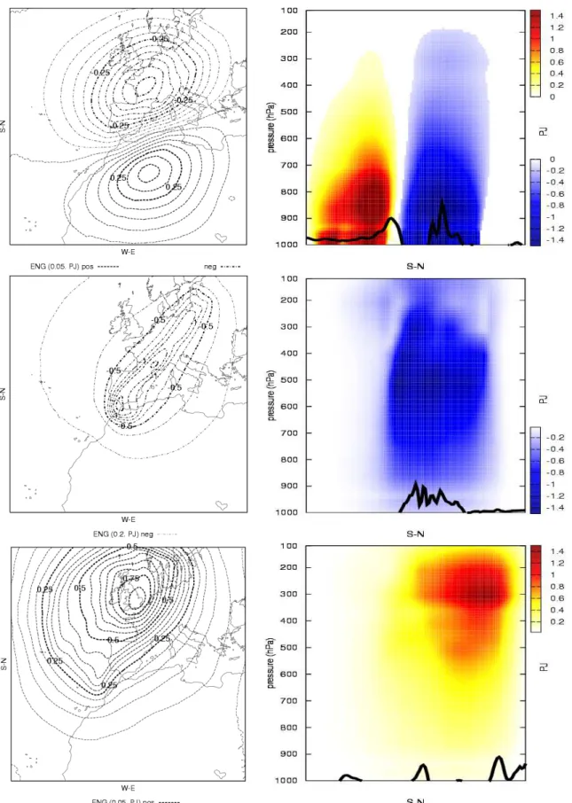
Fig. 6. Surface thermal anomaly defined as ErPVpTerm (top; yellow-red, positive values; white-blue, negative values), Upper level PV perturbation (300 hPa) related to upper level trough de-fined as ErPVp01 (middle), Upper level PV perturbation (300 hPa) related to North Atlantic High defined as ErPVpHigh (bottom), dif-ferent scales are used. Solid lines show difdif-ferent vertical cross sec-tions.
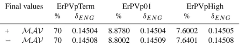
Table 1. Percentage of modifications of the Newtoninan-obtained inverted fields of each anomaly (%) used to modify the initial conditions.
Mean absolute variation of the total energy (MAV) introduced on the initial conditions (+, increasing case; −, decreasing case).
Final values ErPVpTerm ErPVp01 ErPVpHigh % δEN G % δEN G % δEN G
+ MAV 70 0.14504 8.8780 0.14504 7.6002 0.14505
− MAV 70 0.14508 8.8002 0.14509 7.6401 0.14508
condensation. The increase in temperature at mid levels en-hances the stability beneath, which is reflected as positive PV generation (Hoskins et al., 1985; Davis and Emanuel, 1991). However, low-level (p>500 hPa) and moist (RH>70%) ini-tial PV anomalies did not play an important role in prelimi-nar simulations (not shown). This might be due to the fact that the cyclone was formed above the dry and hot Saha-ran desert and a deep convection was developed when the cyclone reached the sea (18 h later than the time when the modification of initial conditions was done).
Selected anomalies are morphologically and spatially dif-ferent (see Fig. 6). The modification of the model initial con-ditions derived from these might be significantly different. In order to compare the roles of the PV anomalies, a “normal-isation” of the perturbation should be done. Then one could be sure that the total amount of change introduced by means of the inverted fields remains constant among the simulations initially, independent of the size and strength of the anomaly. Thus, the results can be adequately intercompared: the non-linear evolution of the atmosphere will show the sensitivity of the event to changes in the initial conditions of the simu-lations.The
PV Inversion technique applied at each PV anomaly pro-duces three-dimensional balanced fields (geopotential, tem-perature, stream function/horizontal wind). The inversion of the equations is numerically done through the overrelax-ation method. For more details, refer to Davis and Emanuel (1991). The modification of the initial conditions will be done by a substraction of a percentage of these inverted fields. Since the inverted fields are obtained for the entire space, the normalisation or quantification of the perturbation requires a three-dimensional variable, and since PV inverted fields represent all atmospheric variables (except humidity), the index used for the normalisation should be a combina-tion of these variables. The total energy (Bluestein, 1992) has been chosen as a plausible function. Using the energy, an energy-derived dynamical study of each anomaly can be accomplished. This is possible since total energy can be split into three components: kinetic (δEN Gkin), potential (δEN Gpot) and internal energy (δEN Gint). The grid point energy (EN G) is obtained from the integration of the volu-metric density of energy (δEN G) across the volume of the grid point (δV, see Eq. 1)
EN G = δEN GkinδV + δE N GpotδV + δE N GintδV
δE N Gkin= 1 2kvk 2ρ = 1 2(u 2+v2)ρ δE N Gpot=gHρ δE N Gint=CvT ρ δV = ds 21p ρg , (1)
where kvk, wind speed; ρ, density; g, gravity; H , geopoten-tial height; Cv, heat capacity at constant volume; T ,
temper-ature; ds2, areal size of the grid point; 1p, pressure variation between bottom and top of the grid cell.
PV inverted fields used to modify the initial conditions im-ply a change in the total amount of energy in the atmospheric domain of the simulation. In this study that change will be computed as the mean absolute variation of the total energy (MAV, Eq. 2)
MAVχ =
N i,Nj,N kX i,j,k
|χmod(i, j, k) − χref(i, j, k)|
N i × Nj × N k , (2)
where χmod(i, j, k) is the modified energy at each grid point;
χref(i, j, k) the unperturbed field and Ni, Nj, Nk, the number
of grid points in each direction.
The proposed normalisation of the perturbations is realised by imposing the same energy variation in the initial condi-tions for each anomaly. Although each PV anomaly will be modified with a different pattern, the environment and the to-tal amount of introduced/removed energy is forced to be the same. This condition will be condensed on a given percent-age of the inverted balanced fields to be used to modify the initial conditions.
In the November 2001 case, the Upper level disturbances (ErPVp01 and ErPvpHigh) are clearly stronger than the face thermal one (ErPVpTerm in Fig. 6). Therefore, the sur-face thermal anomaly will be used as a reference. Thus, 70% of the PV inverted fields from the surface thermal anomaly will determine a fixed energy perturbation of about 0.145 PJ (PJ=1015J) on the initial conditions. This energy value is used to fix the perturbations when the upper level anoma-lies are used. A Newtonian or Bisection iterative numerical
method (Arfken, 1985) is used. This method is used to obtain the percentage of the inverted fields from ErPVp01 and Er-PVpHigh that preserves the same amount of energy variation as the ErPVpTerm modification. The results of this numeri-cal computation are summarised in Table 1.
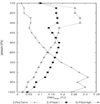
Different perturbation energy profiles are derived from the anomalies, as it is shown in Fig. 7. ErPVpTerm in-fluences much more the low levels, whereas ErPVp01 and ErPVpHigh influence strongly the upper levels. ErPVp01 is more evenly distributed in the vertical than ErPVpHigh, depicting the structural differences between troughs or cut-off lows and blocking anticyclones (Hoskins et al., 1985; Thorpe, 1986).
Figure 8 gives spatial information on the impact of each anomaly over the initial conditions. It shows the three-dimensional effect on the total energy. ErPVpTerm extracts and adds energy to the environment. Since ErPVpTerm anomaly is aimed at capturing the surface baroclinicity of the initial environment, it has been constructed with both the positive and negative surface thermal anomaly. Perturbations carried out with a positive(negative) thermal anomaly is re-lated to a decrease(increase) in the total energy. Upper level positive(negative) potential vorticity perturbations are related to a decrease(increase) in the total energy (see Fig. 9). Re-sults of ErPVpTerm anomaly (top panel in Fig. 9) do not show an upward decrease profile as the MAV value (dash and cross line in Fig. 7). This is because the ErPVpTerm is based on both positive and negative thermal anomalies (top Fig. 6). As a result, the inverted fields increase/decrease the energy of the environment. Figure 9 gives the averaged to-tal variations of this energy (thus allowing compensation be-tween terms); meanwhile, in the MAV computation this is not allowed, since absolute values are used.
The perturbation energy partition among kinetic, potential and internal for each anomaly is shown in Fig. 9. ErPVp-Term is related to a variation in the internal and potential energies. The effect is almost constant at all vertical levels. ErPVp01 and ErPVpHigh energy contributions are broadly similar. These anomalies have an important effect on the po-tential and internal energy, with the maximum energy varia-tion found at upper levels. Significant perturbavaria-tions of the ki-netic energy are also found at upper levels, where the anoma-lies are defined. ErPVp01 has the highest impact on the po-tential energy, while ErPVpHigh has the highest impact on the internal energy.
However, one cannot infer directly that an increase or de-crease in the available energy to the environment will pro-duce deeper or weaker systems. As it has been shown, in-creasing the upper level positive PV anomaly induces a sig-nificant decrease in the potential and internal energy, despite the fact that a strong upper level positive PV anomaly is usually related to strong cyclogenesis (Pettersen and Sme-bye, 1971; Hoskins et al., 1985). Energy impacts are shown as horizontally averaged values. Any information about changes in morphology and position of the features in the
Fig. 7. Vertical profile of the mean absolute energy variation (MAV) of the initial conditions according to the positive percent-age found for each anomaly. ErPVpTerm (cross), ErPVp01 (filled square), ErPVpHigh (triangles). Note that the same area is enclosed by each curve (same total energy).
fields, from which genesis and maintenance of the atmo-spheric systems are explained, is not provided. Energetical implications for the baroclinic instability (Robinson, 1989) is out of scope of this study.
4 Results of the simulations
The sensitivity to changes in the initial conditions will be derived from the differences between the collection of sim-ulated cyclones. The impacts on the simsim-ulated trajectories, central pressure value and central vorticity of the cyclones will be examined. Besides, a short description of the upper level vortex (C0) properties and evolutions will be given. The computation of the vorticity characteristics of the cyclones follow the criteria of Campins et al. (2000), where a 200 km gridlength mesh is used.
Generally, simulated cyclones show a symmetric response between positive and negative modifications of the initial fields. That is, the two cyclones show the same variations, with opposite sign, from the control one (not shown). These differences are not very strong, owing to the small degree of modification introduced.
4.1 Effects of the ErPVpTerm perturbation
The modification of the environmental baroclinicity (± ErPVpTerm) reveals significant variations with respect to the
Fig. 8. Energy variations (PJ) introduced after the modification of the initial conditions (10 November 2001 at 00:00 UTC), according to each
positive percentage of modification of the PV Inverted fields of each anomaly; ErPVpTerm (top), ErPVp01 (middle), ErPVpHigh (bottom). At 500 hPa (left) and following vertical cross sections defined at Fig. 6 (right).
Fig. 9. Vertical profiles of the horizontally averaged total variations of energy (in PJ) according to the positive percentage of modification
for each anomaly. Total energy variation (solid line, filled circles), Potential energy (EN Gpot, dotted line with squares), Kinetic energy
(EN Gin, dashed line with crosses), Internal energy (EN Gint, dot-dash line with triangles). ErPVpTerm (top), ErPVp01 (bottom left),
ErPVpHigh (bottom right).
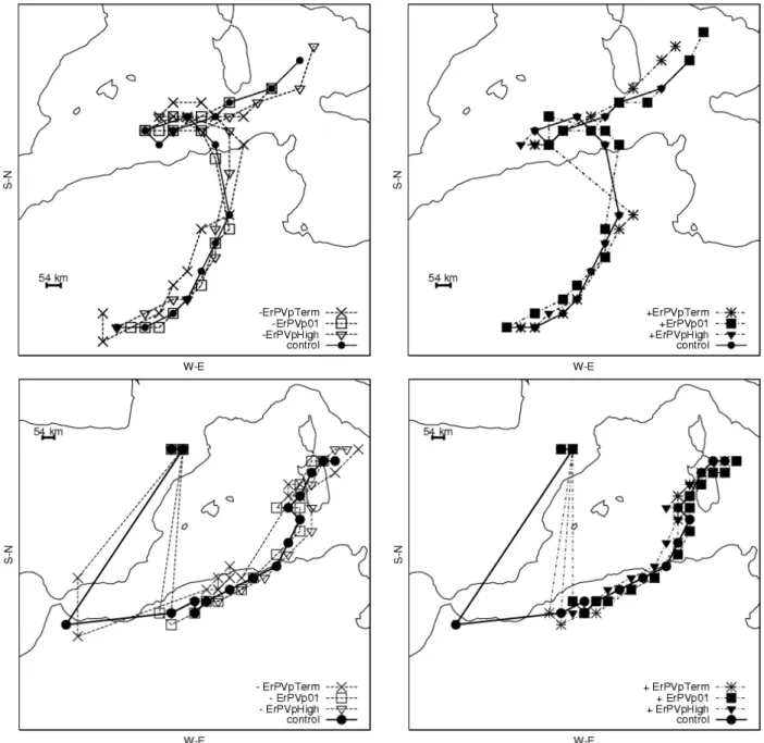
control simulation during the initial and last phases of the cyclone evolution. These differences are the largest ones among the entire set of perturbations at the initial phase of the simulations. According to the results, the differences in the initial position of the cyclone are about 480 km (see Fig. 11), and for the initial central pressure value of the cy-clone approx. ±4 hPa (see Fig. 12). At the same time, the simulated cyclones show strong variations in their vorticity (about ±5 s−1 at 200 km gridmesh point, in Fig. 14). As a
result of the change in the initial position of the cyclone, the interaction between the upper and low level disturbances has also changed (the relative phase between the disturbances is significantly changed in comparison to the other simulations, Fig. 13).
In the −ErPVpTerm(+ErPVpTerm) case (perturbation of the initial conditions by subtracting(increasing) the fields re-lated to the horizontal thermal anomaly) the initial trajectory of the cyclone is clearly different from the control one (see
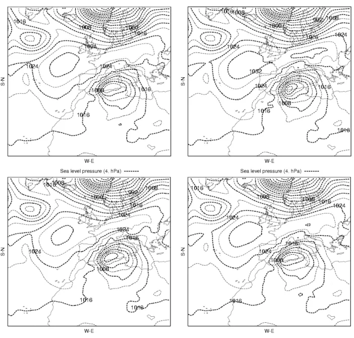
Fig. 10. Sea level pressure at the mature state of the cyclone (11 November 00:00 UTC). Lines every 2 hPa. For the control simulation (top
left), +ErPVpTerm (top right), +ErPVp01 (bottom left) and +ErPVpHigh (bottom right).
the two dashed lines with crosses in Fig. 11). The mature cyclones at 11 November 00:00 UTC show the largest vari-ations with the control one: on the lowest central pressure value (±6 hPa, Fig. 12), the relative distance with C0 (be-tween 100-200 km in Fig. 13) and the central value of the upper level trough C0 about 1 with the PVU less than in the control one, (Fig. 13). ErPVpTerm perturbations have a deep impact when the cyclone crosses the Atlas moun-tains, modifying the relation between the cyclone and the upper level trough. This is shown in the phase-relative-distance (Fig. 13). As result, the perturbed cyclone from
−ErPVpTerm changes to a negative relative phase (C0 is lo-cated in an eastern position relative to the cyclone) 9 h later than the +ErPVpTerm cyclone.
Initially, the C0 simulated from the ± ErPVpTerm pertur-bations is similar with respect to the control one. However, at the mature state of the cyclone, C0 values are about 1 PVU lower (see Fig. 13). The strong differences may be related to the change in the phase of the mutual interaction with the surface cyclone, attributed to the baroclinic deepening pro-cesses. This aspect is also reflected in the +ErPVpTerm cy-clone simulation. The cycy-clone exhibits a stronger vorticity
Fig. 11. Top panels: Trajectories of the cyclone obtained from the initially perturbed simulations. Bottom panels: Trajectory of C0 for the
dif-ferent simulations. For the negative modifications (left), for the positive modifications (right). According to values on Table 1. −ErPVpTerm (simple cross), +ErPVpTerm (full cross), −ErPVp01 (empty square), +ErPVp01 (filled square), −ErPVpHigh (empty triangle), +ErPVpHigh (filled triangle).
than the control one (see Fig. 14), associated with a deeper cyclone and a stronger North Atlantic high, which results in much stronger surface pressure gradients (see Fig. 10). Dur-ing the dissipative phase of the cyclone (from 11 Novem-ber at 12:00 UTC to 12 NovemNovem-ber at 00:00 UTC), the dif-ferences regarding the control cyclone become strong. The final position is clearly shifted about 54 km from the con-trol one in both cases (Fig. 11), the central pressure value is changed by about ±2 hPa (Fig. 12), and the final values of C0 are stronger (about ±1.5 PVU, Fig. 13). At the end of
the simulated period a lower vorticity of the −ErPVpTerm cyclone is obtained due to the smaller dimensions of the cy-clone, in comparison to the +ErPVpTerm one (not shown). The strongest deepening of the cyclone occurred between 10 November at 18:00 UTC and 11 November at 06:00 UTC (see Fig. 12). In contrast with the strong sensitivity to the ErPVpTerm anomaly, the growth rate of the cyclone does not vary significantly (about −8 hPa/12 h in positive case and
Fig. 12. Labels as in Fig. 11, but left panel: evolution of the central pressure of the cyclone. Right panel: evolution of the central pressure of
the cyclone rescaled to control simulation results.
Fig. 13. Labels as in Fig. 11, but left panel: evolution of the C0 central value (PVU). Right panel: Evolution of the relative distance (km)
between C0 and cyclone, positive(negative) sign denotes eastward(westward) relative position of the cyclone (starting date on 10 November at 12:00 UTC).
4.2 Effects of the ErPVp01 perturbation
The cyclone simulated through the ±ErPVp01 perturbations reveals significant impacts on the upper level trough. The effects are most notable during the mature state of the
clone, on 11 November at 00:00 UTC. The simulated cy-clones and the C0 centres describe similar trajectories as the control ones (see lines with squares in Fig. 11). However, the evolution of the central surface pressure values and the C0 magnitudes have been changed (see lines with squares in
Fig. 14. Labels as in Fig. 11, but left panel: evolution of the depth of the cyclone rescaled to control simulation results (defined as the first
minimal vorticity value above the centre of the cyclone, left). Right panel: evolution of the vorticity of the cyclone at a distance of 200 km (defined like in Campins et al., 2000). Each figure has been temporally filtered through a mobile-average filter of 3 time-points.
Figs. 12, 13). Low differences are observed between the fi-nal PV values of C0, between the +ErPVp01 and −ErPVp01 cases (Fig. 13), probably due to diabatic influences.
Initially, the perturbation of ErPVp01 is localized at up-per levels, where the trough is altered (central pressure of the cyclones for ±ErPVp01 cases are initially only ±1 hPa different than the control one). During the initial phase, the cyclones preserve similar vorticities (see Fig. 14), but they change significantly their dimensions (not shown). A stronger or weaker upper level PV vortex does not produce any strong effect on the trajectory of the disturbances (simi-lar trajectories as the control one are obtained; see Fig. 13). However, a weaker upper level disturbance (−ErPVp01 case) decreases the upper-low level interaction and this is depicted as a shallower mature cyclone. With a stronger upper level trough (+ErPVp01 perturbation) the cyclone moves faster than the control one (Fig. 11). Significant geostrophic vortic-ity differences are obtained at the mature stage of the cyclone (11 November at 00:00 UTC, Fig. 14), as a reflection of the changes in the vorticity advections due to a stronger(weaker) upper level trough. In the last phase of the evolution of the cyclone, the C0 value is similar to the control one, but cen-tral pressure values of the cyclone are clearly different (about
±2 hPa), possibly related to changes in the relative phase be-tween C0 and the cyclone at this ending phase. As for the ErPVpTerm anomaly simulations, small differences between the positive/negative cases in the maximum growth rate of the cyclone are also observed for this anomaly.
4.3 Effects of the ErPVpHigh perturbation
The cyclones obtained in the simulations with the Er-PVpHigh anomaly present the lowest sensitivities. The dif-ferences with respect to the control simulation are rather low until the last phase of the cyclone. The largest variations are obtained in the −ErPVpHigh case. A weaker North Atlantic anticyclone (as a result of the -ErPvpHigh initial perturba-tion) can help create a faster movement of the Mediterranean disturbance, owing to a weaker blocking of the anticyclone. Final values of the C0 centre and the relative distances be-tween the low and upper level disturbances do not differ from the control one (see Fig. 13), but final phase trajectories are significantly shifted from the control one (see lines with tri-angles in Fig. 11).
5 Conclusions
Piecewise PV Inversion techniques, combined with per-turbed numerical simulations, have been used as a tool to dynamically study various features of atmospherics systems. These techniques can offer useful information about mecha-nisms and roles of a wide range of features involved in the lifecycle of the disturbances. Although numerical solutions to well-defined inversion equations are determined, some un-certainties and subjectivities arise in its application. Some of these case-dependent aspects are: computation of a ref-erence state from which to define the PV anomalies (zonal mean, temporal mean, number of members to establish an
average, etc.), morphology and magnitude of the anomalies, and degree of modification of the initial conditions. In the present study an objective procedure has been proposed as a method to quantify the latter aspect of the technique. In this way, one can diminish the ambiguity on the use of the PV Inversion technique applied to modify the initial conditions of numerical simulations.
It is proposed to use the total Mean Absolute Variation (MAV) of energy introduced, due to the modification of the initial conditions. The Root Mean Square Variation (RMSV) could have been proposed, but by squaring the values, contributions of big and small energetic variation val-ues are differently, weighted in the RMSV calculation. The partition of the energy into mechanical, internal and kineti-cal energies can be useful information from which a deeper understanding of the role of the collection of features can be obtained.
The 9–12 November 2001 Mediterranean cyclone has been studied in terms of its sensitivity to changes in the ini-tial conditions due to three PV anomalies: the surface ther-mal another-maly related to the origin of the cyclone and the baroclinic initial conditions of the environment; the upper level trough related to the baroclinic growth mechanism of the cyclone; the upper level North Atlantic high pressure zone related to the environmental conditions of the upper tro-posphere. The anomalies show different morphologies and intensities, but since the energy-quantification of the initial modification has been applied, sensitivity results might be only attributed to the dynamical role of the anomalies. The surface thermal anomaly is revealed as the most important feature of the initial conditions for the cyclogenesis. A sig-nificant effect on the initial central pressure of the cyclone and a weak effect on its initial position are shown. Both have a strong effect on the resultant evolution of the case. The sensitivities to changes in the initial conditions due to the up-per level disturbances are also important. Nevertheless, the initial impact on the structure of the cyclone is lower than for the thermal anomaly, but in later stages of the episode the impact becomes the strongest. The effects of changes in the initial conditions associated with the North Atlantic high are weak. However, in the last phase of the cyclone evolu-tion, the initial perturbations show a notorious impact on the trajectory of the cyclone.
The sensitivity results are strongly affected by the baro-clinic mechanism. It is illustrated that the diversity of simu-lated cyclones can be mainly explained as a function of the changes in the vertical tilt between the upper level trough and the surface disturbance. The sensitivity test to the in-crease(decrease) in the surface thermal anomaly shows that with similar values of the upper level disturbance, changes in the relative position and central pressure value of the sur-face disturbance generates deeper(weaker) and faster(slower) evolution of the simulated cyclone. This case also empha-sises the mutual interaction between anomalies, in the sense that the thermal anomaly perturbation does not affect the
ini-tial structure and intensity of the upper level disturbance, but during the simulated period, the upper level disturbance strength clearly differs between both experiments. The upper level disturbance perturbations modify both the initial cen-tral value of the cyclone and the upper level trough, but only slightly modify the relative distance between both features. These variations generate a strongly varied evolution of the cyclone. Finally, the North Atlantic high does not exhibit a significant role on the upper level disturbance, on the surface cyclone strength or on the relative position between distur-bances. However, the small perturbations on the relative po-sition between the upper and low level disturbances seem to be enough to originate significantly different final cyclones.
Finally, the proposed quantification method of the piece-wise PV inversion derived perturbations can be applied as a general methodology in dynamic meteorology. The applica-tion to various events would allow an objective intercompar-ison between cases, independent of the morphology, charac-teristics and origin of the selected anomalies. This method of quantification could contribute to the PV study and analysis based on the most important features involved in the evolu-tion of the cyclones or other atmospheric phenomena.
Acknowledgements. Support from MEDEXIB (REN 2002-03482)
and PRECIOSO (CGL2005-03918/CLI) projects and PhD grant BES-2003-0696 (all from the Spanish “Ministerio de Educaci´on y Ciencia”) are acknowledged. V. Homar for the discussions and commentaries is also acknowledged. J. Campins for the commen-taries and help. ´A. Luque for the satellite image.
Topical Editor U.-P. Hoppe thanks two anonymous referees for their help in evaluating this paper.
References
Arfken, G.: Mathematical Methods for Physicists, 3rd ed., Orlando, FL: Academic Press, 1985.
Argence, S., Lambert, D., Richard, E., S¨ohne, N., Chaboureau, J.-P., Cr´epin, F., and Arbogast, P.: High resolution numerical study of the Algiers 2001 flash flood: sensitivity to the upper-level po-tential vorticity anomaly, Adv. Geosci., 7, 251–257, 2006, http://www.adv-geosci.net/7/251/2006/.
Bleck, R.: Depiction of upper/lower vortex interaction associated with extratropical cyclogenesis, Mon. Weather Rev., 118, 573– 585, 1990.
Bluestein, H. B.: Synoptic-Dynamic Meteorology in Midlatitudes. Volume 1, Oxford university press, Inc., 1992.
Bretherton, F. P.: Critical layer instability in baroclinic flows, Q. J. Roy. Meteor. Soc., 92, 325–334, 1966.
Campins, J., Genov´es, A., Jans`a, A., Guijarro, J. A., and Ramis, C.: A catalogue and a classification of surface cyclones for the western Mediterranean, Int. J. Climatol., 20, 969–984, 2000. Campins, J., Jans`a, A., and Genov´es, A.: Three-dimensional
struc-ture of western Mediterranean cyclones, Int. J. Climatol., 26, 323–343, 2006.
Charney, J. G.: The use of primitive equations of motion in numer-ical prediction, Tellus, 7, 22–26, 1955.
Davis, C. A. and Emanuel, K. A.: Potential vorticity diagnostics of cyclogenesis, Mon. Weather Rev., 119, 1929–1953, 1991. Davolio, S. and Buzzi, A.: A nudging scheme for the assimilation
of precipitation data into a mesoscale model, Weather Forecast., 19, 855–871, 2004.
Grell, G., Dudhia, J., and Stauffer, D.: A description of the fifth-generation Penn State/NCAR mesoscale model (MM5), NCAR Technical Note, NCAR/TN-398+STR, 117pp, 1994.
Gyakum, J. R.: On the Evolution of the QE II Storm. II: Dynamic and Thermodynamic Structure, Mon. Weather Rev., 111, 1156– 1173, 1983b.
Hakim, G. J., Keyser, D., and Bosart, L. F.: The Ohio valley wave-merger cyclogenesis event of 25–26 january 1978. Part II: Diag-nosis using quasigeostrophic potential vorticity inversion, Mon. Weather Rev., 124, 2176–2205, 1996.
Homar, V., Ramis, C., and Alonso, S.: A deep cyclone of African origin over the Western Mediterranean: diagnosis and numerical simulation, Ann. Geophys., 20, 93–106, 2002,
http://www.ann-geophys.net/20/93/2002/.
Homar, V., Romero, R., Stensrud, D., Ramis, C., and Alonso, S.: Numerical diagnosis of a small, quasi-tropical cyclone over the western Mediterranean: Dynamical vs. boundary factors, Q. J. Roy. Meteor. Soc., 129, 1469–1490, 2003.
Horvath, K., Fita, L., Romero, R., and Ivancan-Picek, B.: A numer-ical study on the first phase of a deep Mediterranean cyclone: Cyclogenesis in the lee of the Atlas Mountains, Meteorologische Z. 1, 15, 133–146, 2006.
Hoskins, B. J., McIntyre, M. E., and Robertson, A. W.: On the use and significance of isentropic potential vorticity maps, Q. J. Roy. Meteor. Soc., 111, 877–946, 1985.
Huo, Z., Zhang, D.-L., Gyakum, J. R., and Stainforth, A. N.: A diagnostic analysis of the superstorm of march 1993, Mon. Weather Rev., 123, 1740–1761, 1995.
Huo, Z., Zhang, D.-L., Gyakum, J. R., and Stainforth, A. N.: Inter-action of potential vorticity anomalies in extratropical cyclogen-esis. Part I: Static Picewise Inversion, Mon. Weather Rev., 127, 2546–2561, 1999a.
Huo, Z., Zhang, D.-L., Gyakum, J. R., and Stainforth, A. N.: Inter-action of potential vorticity anomalies in extratropical cycloge-nesis. Part II: Sensitivity to initial perturbations, Mon. Weather Rev., 127, 2563–2575, 1999b.
Kuo, Y. A., Shapiro, M. A., and Donall, E. G.: The interaction between baroclinic and diabatic processes in a numerical simula-tion of a rapidly intensifying extratropical marine cyclone, Mon. Weather Rev., 119, 368–384, 1991a.
Kuo, Y.-H., Reed, R. J., and Low-Nam, S.: Effects of surface en-ergy fluxes during the early development and rapid intensifica-tion stages of seven explosive cyclones in the western Atlantic, Mon. Weather Rev., 119, 457–476, 1991b.
Pettersen, S. and Smebye, S. J.: On the development of extratropical cyclones, Q. J. Roy. Meteor. Soc., 97, 457–482, 1971.
Reed, R. J., Stoelinga, M. T., and Kuo, Y.-H.: A model-aided study of the origin and evolution of the anomalously high potential vor-ticity in the inner region of a rapidly deeping marine cyclone, Mon. Weather Rev., 120, 893–913, 1992.
Robinson, W. A.: On the structure of potential vorticity in baroclinic instability, Tellus, 41A, 275–284, 1989.
Romero, R.: Sensitivity of a Heavy Rain producing Western Mediterranean cyclone to embedded Potential Vorticity anoma-lies, Q. J. Roy. Meteor. Soc., 127, 2559–2597, 2001a.
Sanders, F. and Gyakum, J. R.: Synoptic-Dynamic climatology of the ‘Bomb’, Mon. Weather Rev., 108, 1589–1606, 1980. Thorpe, A. J.: Synoptic scale disturbances with circular symmetry,
Mon. Weather Rev., 114, 1384–1389, 1986.
Tripoli, G. J., Medaglia, C. M., Dietrich, S., Mugnai, A., Pane-grossi, G., Pinori, S., and Smith, E. A.: The 9–10 November 2001 Algerian Flood: A Numerical Study., B. Am. Meteorol. Soc., 86, 1229–1235, 2005.
![Fig. 3. Control simulation results. Left panel: Evolution of the position of the cyclone (dashed line) and the C0 (slash-dot line), date of position is included ([DD] [HH] )](https://thumb-eu.123doks.com/thumbv2/123doknet/14767319.589094/5.892.108.779.96.442/control-simulation-results-evolution-position-cyclone-position-included.webp)