HAL Id: hal-00317317
https://hal.archives-ouvertes.fr/hal-00317317
Submitted on 8 Apr 2004
HAL is a multi-disciplinary open access
archive for the deposit and dissemination of
sci-entific research documents, whether they are
pub-lished or not. The documents may come from
teaching and research institutions in France or
abroad, or from public or private research centers.
L’archive ouverte pluridisciplinaire HAL, est
destinée au dépôt et à la diffusion de documents
scientifiques de niveau recherche, publiés ou non,
émanant des établissements d’enseignement et de
recherche français ou étrangers, des laboratoires
publics ou privés.
Spatio-temporal patterns of seasonal rainfall in Spain
(1912-2000) using cluster and principal component
analysis: comparison
D. Muñoz-Diaz, F. S. Rodrigo
To cite this version:
D. Muñoz-Diaz, F. S. Rodrigo. Spatio-temporal patterns of seasonal rainfall in Spain (1912-2000) using
cluster and principal component analysis: comparison. Annales Geophysicae, European Geosciences
Union, 2004, 22 (5), pp.1435-1448. �hal-00317317�
SRef-ID: 1432-0576/ag/2004-22-1435 © European Geosciences Union 2004
Annales
Geophysicae
Spatio-temporal patterns of seasonal rainfall in Spain (1912–2000)
using cluster and principal component analysis: comparison
D. Mu ˜noz-D´ıaz and F. S. Rodrigo
Department of Applied Physics, University of Almer´ıa, La Ca˜nada de San Urbano, s/n, 04120, Almer´ıa, Spain Received: 20 May 2003 – Revised: 19 December 2003 – Accepted: 23 January 2004 – Published: 8 April 2004
Abstract. In this work, cluster and principal component
analysis are used to divide Spain in a limited number of cli-matically homogeneous zones, based on seasonal rainfall for 32 Spanish localities for the period 1912–2000. Using the hierarchical technique of clustering Ward’s method, three clusters have been obtained in winter and spring, and four clusters have been obtained in summer and autumn. Results are similar to those obtained by applying principal compo-nent analysis. Centroid series of each cluster and principal component series of each EOF have been compared to ana-lyze the temporal patterns. The comparison of both methods indicates that cluster analysis is suitable to establish spatio-temporal patterns of seasonal rainfall distribution in Spain.
Key words. Meteorology and atmospheric dynamics
(cli-matology; precipitation; general or miscellaneous)
1 Introduction
The spatial grouping of observation sites is a common prac-tice in climatology. In general, such grouping provides a convenient way to summarize climatic data in a concise man-ner (DeGaetano, 2001). Cluster analysis (CA) is one of the most useful tasks in the data mining process for discovering groups and identifying interesting patterns in the underlying data (Halkidi et al., 2001). It has come to be recognized as an effective statistical tool to deal with tasks for grouping stations into climatologically homogeneous regions (DeGae-tano and Shulman, 1990; Ahmed, 1997; DeGae(DeGae-tano, 2001), or for grouping time periods into clusters that reflect the oc-currence of weather events or patterns (Ramos, 2001). The purpose of CA is to place objects into groups suggested by the data, not defined previously, so that objects in a given cluster tend to be similar to each other in some sense, and objects in different clusters tend to be dissimilar.
Correspondence to: F. S. Rodrigo (frodrigo@ual.es)
The initial raw data consists of a pxn matrix X, that can be thought of n points in a p-dimensional space. The term “variable” is used for denoting the column vectors, and the term “observation” is used for denoting the row vectors. The most basic stage before applying a clustering algorithm is to establish a numerical similarity or dissimilarity measure-ment to characterize the relationships among the data. Eu-clidean distance is the most commonly used measure, al-though many other distance measurements exist (Gong and Richman, 1995).
Consider a pxn matrix X in a p-dimensional space. The Euclidean distance between the variables Xiand Xj is given
by
dij = [(Xi−Xj)T(Xi−Xj)]1/2, (1) assuming that the p observations are independent. The range of Euclidean distance is from 0 (identical vectors or vari-ables) to +∞ (vectors without relationship). The squared Euclidean distance is often used with similar results.
There are two main types of cluster techniques: divisive and hierarchical (Kaufman and Rousseuw, 1990). The ob-jective of the divisive technique is to separate a set of objects into consistent groups. Each object is placed in one and only one cluster. The preliminary assignation of the objects to one cluster could be done using a random partition and then the objects are transferred from one cluster to another un-til reaching the position in which the similarity is greatest. In the hierarchical technique, the objects are progressively aggregated until they are joined into a single cluster. Each object begins in a cluster itself. Then the closet clusters are merged to form a new cluster that replaces the two old clus-ters. Merging of the two closest clusters is repeated until only one cluster is left.
Most commonly implemented CA procedures are hierar-chical (Wilks, 1995). The purpose is to form each possible number of groups n, n-1, . . . , 1, in a manner to minimize the loss of information. The first step is to combine two clusters P and Q, whose fusion yields the least increase in the sum of squares within clusters distance from each individual to
1436 D. Mu˜noz-D´ıaz and F. S. Rodrigo: Spatio-temporal patterns of seasonal rainfall in Spain (1912–2000) 23 Figure 1 AB A BA B BU CC CR V CU Al LC H HU J LO M MA MU P SA SF SS S SC SG SE SO TO TT VA Z
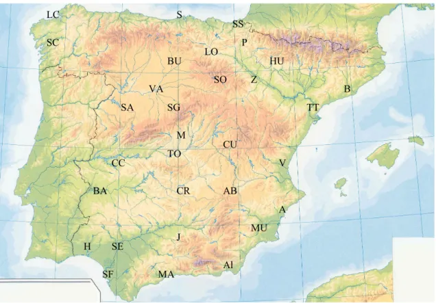
Fig. 1. Map of the study area (station code in Table 1).
the centroid of its present cluster n, resulting in n-1 groups. The next step is to examine the n-1 group to determine if a third member should be linked with the first pair or another pairing made, in order to secure the optimum value of the objective function for n-2 groups. This process continues until all stations are clustered in one group and all the cli-matic differences are concealed (Ahmed, 1997). There are different hierarchical methods, according to the aggregation criteria. In this work, the method used is Ward’s method of clustering.
Most of the multivariate methods use the hypothesis of normality for the original data. However, clustering algo-rithms generally do not restrict the input database to particu-lar statistical distributions, because CA is more an objective method to quantify the characteristics of a set of observa-tions than a inference statistical tool. Therefore, the require-ments of normality and homoscedasticity, important in other multivariate techniques, are not necessarily applied in CA (Mart´ınez Arias, 1999). Rainfall series in the Iberian Penin-sula are best modelled by skewed distribution functions, as the gamma distribution function (Lana and Burgue˜no, 2000). In consequence, CA is especially interesting in studying rain-fall series and its spatio-temporal variability in Spain.
In this paper, a hierarchical technique of clustering (Ward’s method) is used to divide the Iberian Peninsula area in a limited number of climatically homogeneous zones based on the meteorological variable of seasonal rainfall for 32 Spanish localities. The main objective is to compare the results with those of the principal component analysis (PCA),
possibly the most widely used multivariate statistical tech-nique in the atmospheric sciences.
2 Data
The database used in this study comprises seasonal total amounts of precipitation for 32 Spanish localities, covering the Iberian Peninsular area (Fig. 1), except Portugal. They were selected from a set supplied by the Spanish Meteoro-logical Institute (INM), having met quality criteria (Almarza et al., 1996). Most of the stations have not changed their po-sition, but the meta data relative to methods and instruments is known for only a few. Esteban-Parra et al. (1998) anal-ysed the homogeneity of these series by applying absolute and relative homogeneity tests (Thom and Barlett tests), and they concluded that these series are high quality and they do not possess inhomogeneity problems. Table 1 summarises the geographical data of the meteorological stations (altitude above sea level, latitude and longitude). In this study we se-lected the common period of timeseries (1912–2000) for all meteorological stations, to obtain a regionalization of sea-sonal rainfall distribution patterns in the Iberian Peninsula.
Variables are usually standardized before applying CA, to eliminate possible scale effects. For each station, total sea-sonal rainfall was standardized using 1961–1990 as a refer-ence period, as
zi = xi−xi
σi
where xi is the seasonal rainfall in the season i, xi and σi are the mean value and the standard deviation, respec-tively, of the reference period. This period has been used as a reference period to accomplish the WMO suggestions (Ojo and Afiesimama, 2000). In addition, future projections on climate change (e.g. Hulme and Sheard, 1999) use this period as a reference period and express climate changes as percentages of this period values. The reference pe-riod was compared with the complete pepe-riod and signifi-cant differences were not found. Because normalization is not made using the complete period 1912–2000, the mean value and standard deviation of the zi series are not
nec-essarily equal to 1 and 0, respectively. Seasons consid-ered here are winter (December–January–February), spring (March–April–May), summer (June–July–August), and au-tumn (September–October–November).
3 Methods
3.1 CA (Ward’s Method)
Ward (1963) proposed a very general hierarchical cluster method known as “Ward’s method” or the “minimum vari-ance method”. The Ward’s method calculates the distvari-ance between two clusters as the sum of squares between the two clusters added up over all the variables. At each generation, the within-cluster sum of squares is minimised over all par-titions obtainable by merging two clusters from the previous generation. If Ckand Clare two clusters that merged to form
cluster Cm, the combinatorial formula that defines the
Eu-clidean distance between the new cluster and another cluster Cjis:
dj,m= (nj+nk)dj k+(nj+nl)dj l−njdkl nj+nm
(3) where nj, nk, nl and nm are the number of objects in
clus-ters j, k, l and m, respectively, and dj k, dj land dklrepresent
the distances between the observations in clusters j and k, between j and l, and between k and l, respectively (Ramos, 2001).
Thus, Ward’s algorithm can be implemented through up-dating a stored Euclidean distance between cluster cen-troides. Ward’s method can be quite a versatile technique for CA, even though it has been limited to Euclidean distance (Anderberg, 1973). Although clustering results may be sen-sitive to the chosen method (e.g. average-linkage as opposed to Ward), Blashfield (1976) found that the Ward’s method “clearly obtained the most accurate solutions” among the four hierarchical methods he tested and recommended it to the researchers who wish to use a hierarchical method.
The progress and intermediate results of a cluster analysis are conventionally illustrated using the dendogram or “tree” diagram, a bidimensional figure that represents the sequence and the distance at which the observations are clustered. Cli-matic groups can be selected from the clusters of the den-dogram. Beginning with the “twigs” at the beginning of the
Table 1. Rainfall data series in Spain for the period 1912–2000. Station (CODE) Altitude (m a.s.l.) Latitude Longitude Albacete (AB) 699 38◦56’00”N 01◦51’00’W Almeria (AL) 21 36◦50’00”N 02◦23’00”W Alicante (A) 82 38◦22’00”N 00◦29’40”W Badajoz (BA) 195 38◦53’00”N 06◦48’00”W Barcelona (B) 94 41◦25’05”N 02◦07’30”W Burgos (BU) 854 42◦22’00”N 03◦38’00”W Caceres (CC) 459 39◦29’00”N 06◦20’15”W Ciudad Real (CR) 629 38◦59’00”N 03◦55’00”W Cuenca (CU) 945 40◦04’00”N 02◦07’00”W Granada (GR) 680 37◦08’00”N 03◦37’00”W Huelva (H) 26 37◦15’00”N 06◦56’00”W Huesca (HU) 542 42◦05’00”N 00◦19’35”W Jaen (J) 510 37◦46’00”N 03◦47’00”W La Coru˜na (LC) 67 43◦22’02”N 08◦25’10”W Logro˜no (LO) 379 42◦28’05”N 02◦26’05”W Madrid (M) 667 40◦24’40”N 03◦40’41”W Malaga (MA) 7 36◦40’00”N 04◦29’00”W Murcia (MU) 75 37◦57’00”N 01◦13’00”W Pamplona (P) 442 42◦49’10”N 01◦38’36”W Salamanca (SA) 782 40◦56’50”N 05◦29’41”W San Fernando (SF) 30 36◦27’00”N 06◦12’00”W San Sebastian (SS) 259 43◦18’24”N 02◦02’22”W Santander (S) 65 43◦27’53”N 03◦49’08”W Santiago Comp. (SC) 260 42◦53’00”N 08◦26’00”W Segovia (SG) 1005 40◦48’00”N 04◦08’00”W Sevilla(SE) 31 37◦25’00”N 05◦53’00”W Soria (SO) 1080 41◦46’00”N 02◦28’00”W Toledo (TO) 540 39◦51’26”N 04◦01’28”W Tortosa (TT) 49 40◦49’14”N 00◦29’14”E Valencia (V) 11 39◦28’48”N 00◦22’52”W Valladolid (VA) 735 41◦46’00”N 04◦46’00”W Zaragoza (Z) 233 41◦39’43”N 01◦00’29”W
analysis, when each of the p observations x constitutes its own cluster, one pair of “branches” is joined at each step as the closest two clusters are merged. The distance between these clusters before they are merged are also indicated in the diagram by the distance of the point of merger from the initial n-cluster stage of the “twigs”.
A CA will produce a different grouping of n observations at each of the n-1 steps. On the first step each observation is a separate group, and on the last step all the observa-tions are in a single group. An important practical problem in cluster analysis is the choice of which intermediate stage will be chosen as the final solution. One decision that must be made concerns the number of clusters to be retained for each method but there are no universally accepted objective techniques by which to accomplish this (Gong and Richman, 1995). Thus, one needs to choose the level of aggregation in the dendogram at which to stop the merging of the cluster. Generally the stopping point will require a subjective choice. A traditional subjective approach for the determination of the stopping level is to inspect a plot of the distances between
1438 D. Mu˜noz-D´ıaz and F. S. Rodrigo: Spatio-temporal patterns of seasonal rainfall in Spain (1912–2000) 24 Di st an ce 0 0,4 0,8 1,2 1,6 2 (X 1000) A AB B AL BA CC CR CU M GR J H MA HU BU LC LO MU TT TO SE SF SC SA SO SG P S SS V VA Z Stage Di st ance 0 10 20 30 40 0 0,4 0,8 1,2 1,6 2 (X 1000) PC number Eige nva lue 0 10 20 30 40 0 4 8 12 16 Figure 2
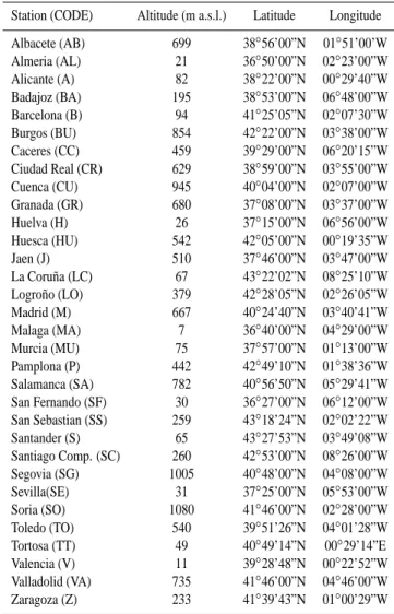
Fig. 2. Dendrogram (top), agglomeration distance plot (middle) and scree plot (bottom) for winter.
merged clusters as a function of the stage of the analysis. When similar clusters are being merged early in the process, these distances are small, and they increase relatively little from step to step. Late in the process there may be only a few clusters, separated by large distances. If a point can be discerned where the distances between merged clusters jumps markedly, the process can be stopped just before these distances become large (Wilks, 1995).
3.2 PCA
PCA is a technique useful for reducing information in a large number of variables, into a smaller set, while losing only a small amount of information. The purpose is to identify the most important correlation structures between a number of variables in order to obtain a description of the major part of the overall variance with few linear combinations based on the original variables.
25 Distance 0 400 800 1200 1600 2000 2400 A AB AL B BA BU CC CR CU GR H HU M J LO MA LC MU TT TO SA SO SG SE SF SC S SS P V VA Z Stage D ist ance 0 10 20 30 40 0 400 800 1200 1600 2000 2400 PC number Ei genval ue 0 10 20 30 40 0 3 6 9 12 15 Figure 3
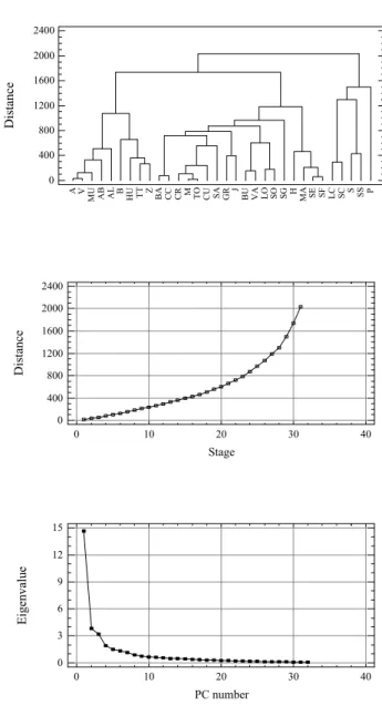
Fig. 3. As Fig. 2, for spring.
There is no single clear criterion that can be used to choose the number of principal components that are best retained in a given circumstance. While the choice of the truncation level can be aided by one or more of the many available selection rules, it is ultimately a subjective choice that will depend in part on the data at hand and the purposes of the analysis. Ac-cording to Rogers (1990) and Rogers and McHugh (2002), the decision regarding how many patterns to retain for rota-tion may be based on scree plots of the eigenvalues. Use of the scree plots requires a subjective judgment about the ex-istence and location of a break in the plotted curve (Wilks, 1995). In making the decision, we identify the location of the first major shelf in the eigenvalues (O’Lenic and Livezey, 1988), wherein the final shelf eigenvalue still accounts for more than 5% of the total unrotated data set variance.
There are methodological differences among PCA studies, often based around the question of whether to apply orthog-onal or oblique rotation to the unrotated eigenvector fields.
Table 2. Percentages of explained variance for each unrotated EOF for seasonal data.
EOFs Winter Spring Summer Autumn
1st 46.80 41.34 30.44 37.60
2nd 14.80 10.74 12.60 12.95
3rd 7.27 9.03 6.76 8.29
4th 4.53 4.26 5.26 5.57
In unrotated analyses the first eigenvector, or empirical or-thogonal function (EOF) accounts for the largest amount of overall data set variance. The major advantage of eigenvec-tor rotation is to obtain a more accurate representation of the dominant spatial modes of the data fields than occurs in the unrotated solutions, although it is achieved by a redistribu-tion of the data set variance contained in the first few unro-tated EOFs (Rogers and McHugh, 2002). In order to obtain statistically robust patterns, orthogonal rotation is performed on a certain number of the unrotated patterns, using a vari-max rotation procedure. Varivari-max defines a simple factor as one with only 1s and 0s in the column. Such a simplification is equivalent to maximising the variance of the squared load-ings in each column (On-Kim, 1970). As a consequence of the rotation of the eigenvectors, a second set of new variables is produced. A number of procedures for rotating the original eigenvectors exist, but all seek to produce what is known as a simple structure in the resulting analysis, if a large number of the elements of the resulting rotated vectors are near zero, and few of the remaining elements correspond to elements that are also not near zero in the other rotated vectors. The re-sult is that the rotated vectors represent mainly the few orig-inal variables corresponding to the elements not near zero, and that the representation of the original variables is split be-tween as few of the rotated eigenvectors as possible (Wilks, 1995). Part of the scientific community advocates the use of rotation fervently, arguing that it is a means with which to diagnose physically meaningful, statistically stable patterns from data. The technique produces compact patterns that can be used for regionalization, that is, to divide an area into a limited number of homogeneous sub-areas (von Storch and Zwiers, 1999). A detailed description of the Varimax method can be found in the statistical textbooks by On-Kim (1970), Preisendorfer (1988) and von Storch and Zwiers (1999).
4 Analysis and results
4.1 Spatial patterns
Figure 2 (top) shows the results of clustering the data cor-responding to winter, using the squared Euclidean distance measure and the Ward’s method. Figure 2 (middle) shows the distance between merged clusters as a function of the stages in the analysis. Subjectively, these distances climb gradually
26 Di st ance 0 400 800 1200 1600 2000 2400 A AB MU AL MA CR TO M CU BA CC GR H SE J SF B Z HU P S SS TT V BU VA SA LO SO SG LC SC Stage Di st ance 0 10 20 30 40 0 400 800 1200 1600 2000 2400 PC number Eige nva lue 0 10 20 30 40 0 2 4 6 8 10 12 Figure 4
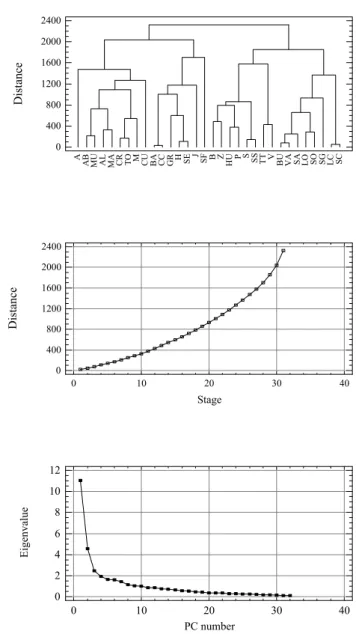
Fig. 4. As Fig. 2, for summer.
until stage 29 or 30, when the distances between combined clusters begin to become noticeably larger. A reasonable in-terpretation of this change in slope is that true clusters have been defined at this point, and that larger distances at later stages indicate mergers of clusters that should be distinct. A plausible point at which to stop the analysis would be after stage 29. This stopping point results in the definition of three clusters on the dendogram. Cluster 1 includes 68.7% of the observations, cluster 2 21.9% and cluster 3 9.4%. Figure 2 (bottom) shows eigenvalues as a function of the EOF number. In this case, three factors have been extracted, the third one accounting for more than 5% of the variance (Table 2). The first three EOFs account for the 68.87% of the total variance. Similar analysis can be seen in Figs. 3 to 5, corresponding to the other seasons of the year. Table 2 shows the percentage of explained variance corresponding to the first four unro-tated EOFs. If the criterium of accounting for more than 5% of the variance is accepted, results indicate that the number
1440 D. Mu˜noz-D´ıaz and F. S. Rodrigo: Spatio-temporal patterns of seasonal rainfall in Spain (1912–2000) 27 Distance 0 300 600 900 1200 1500 1800 A AB AL MA B BA CC GR H CR CU M HU J BU LO LC MU TT V SE SF TO Z SO VA SA SG SC P S SS Stage Di st ance 0 10 20 30 40 0 300 600 900 1200 1500 1800 PC number Eige nva lue 0 10 20 30 40 0 2 4 6 8 10 12 Figure 5
Fig. 5. As Fig. 2, for autumn.
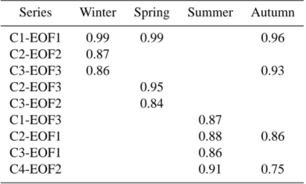
Table 3. Correlation coefficients between centroid time series and principal component time series.
Series Winter Spring Summer Autumn
C1-EOF1 0.99 0.99 0.96 C2-EOF2 0.87 C3-EOF3 0.86 0.93 C2-EOF3 0.95 C3-EOF2 0.84 C1-EOF3 0.87 C2-EOF1 0.88 0.86 C3-EOF1 0.86 C4-EOF2 0.91 0.75
of EOFs to be considered in varimax rotation is 3, 3, 4 and 4 for, respectively, winter, spring, summer and autumn. These numbers coincide with the number of clusters determined from the visual inspection of dendrograms and agglomera-tion distance plots.
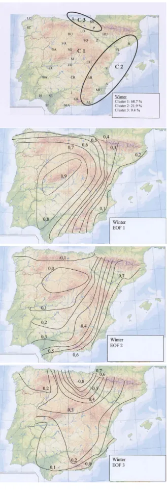
Figures 6 to 9 show the spatial structure detected in data by both methods for each season of the year. In these figures, the top panel shows the spatial grouping detected by CA, and the other panels show the loading factors correspond-ing to each EOF after the varimax rotation is made (4th EOF for summer and autumn not shown). Figure 6, correspond-ing to winter, shows that cluster 1 coincides with the spatial structure of the first EOF, cluster 2 with EOF 2 and clus-ter 3 with EOF 3. Results are similar to the previous analysis (Esteban-Parra et al., 1998; Rodriguez-Puebla et al., 1998). The first EOF and cluster 1 are centred in western Iberia, where rainfall is mainly associated with westerly circulation (Trigo and Palutikof, 2001). The second rotated EOF and cluster 2 are associated with the precipitation regime in the Mediterranean coast, where precipitation is mainly produced by eastern flows (Romero et al., 1999). The third EOF and cluster 3 are associated with rainfall fluctuations in the north-ern coast, where rainfall mainly originated in a meridional north or northwest circulation (Goodess and Jones, 2002).
This pattern is repeated with slight differences in spring (Fig. 7), with the enlargement of the cluster 3 to cover the entire north coast of the peninsula. In this season the to-tal variance explained by the three first unrotated EOFs is slightly minor, a 61.11%. In this case, the correspondences are between cluster 1 and EOF 1 (western Iberia), cluster 2 and EOF 3 (Mediterranean coast), and cluster 3 and EOF 2 (northern coast).
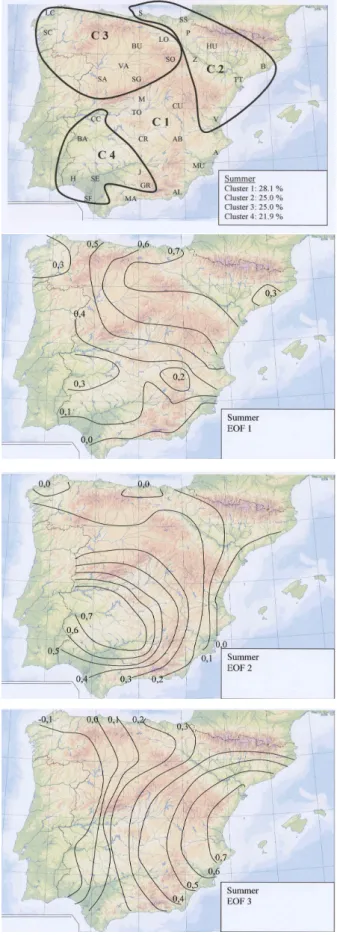
In summer (Fig. 8) this spatial structure seems to break, noticeably in the Mediterranean coast. An explanation of this behaviour may be found in the fact that the northeast region (cluster 2, EOF 1) is affected by the incidence of sum-mertime incursions of maritime air and frontal disturbances around the northern flank of the Mediterranean summer anty-ciclone, while the southeast region (cluster 1, EOF 3), which possesses the lowest average precipitation, is not influenced by this mechanism (Sumner et al., 2001). EOF 2 and clus-ter 4 show a very similar patclus-tern, while EOF 4 (not shown) indicates a sparse pattern, with maxima of the loading fac-tors in the northwest (cluster 3) and southwest areas. CA distinguishes between the northwest and southwest regions, but PCA does not establish this difference clearly.
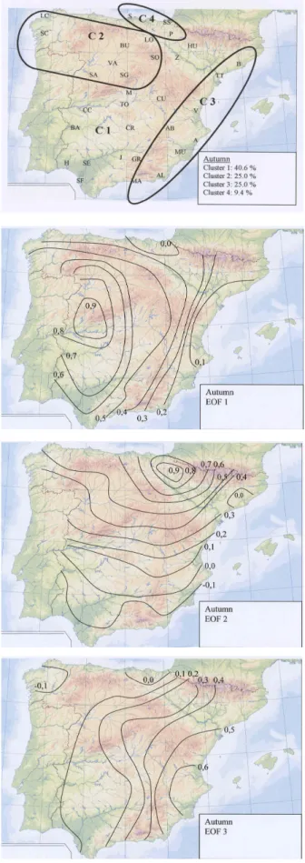
Autumn (Fig. 9) seems a transition season, with four re-gions, but a clear similarity with the winter pattern, and the 64.41% of the total variance explained by the first four un-rotated EOFs. In a certain sense, this pattern reflects the influence of convective and local storms in early autumn, and the influence of westerly circulation types from Octo-ber onwards, showing the transition from summer to winter conditions. Clusters 1 and 2 seem to correspond to EOF 1, cluster 4 to EOF 2, cluster 3 to EOF 3, while EOF 4 (not shown) indicates a very sparse pattern, perhaps indicating the
28 Figure 6
Fig. 6. Regionalization determined by cluster analysis (top panel) and loading factors for the three first rotated EOFs, for winter. In top panel percentage of observations corresponding to each cluster are included.
1442 D. Mu˜noz-D´ıaz and F. S. Rodrigo: Spatio-temporal patterns of seasonal rainfall in Spain (1912–2000)
29 7
Figure 8
Figure 7 Fig. 7. As Fig. 6, for spring.
30 Figure 8
1444 D. Mu˜noz-D´ıaz and F. S. Rodrigo: Spatio-temporal patterns of seasonal rainfall in Spain (1912–2000)
31 Figure 9
32 Year cluster 1 EOF 1 1910 1930 1950 1970 1990 2010 -3 -2 -1 0 1 2 3 -60 -50 -40 -30 -20 -10 0 10 20 30 40 50 60 Year cluster 2 EOF 2 1910 1930 1950 1970 1990 2010 -3 -2 -1 0 1 2 3 -20 -15 -10 -5 0 5 10 15 20 Year cluster 3 EOF 3 1910 1930 1950 1970 1990 2010 -4 -3 -2 -1 0 1 2 3 4 -25 -20 -15 -10 -5 0 5 10 15 20 25 Figure 10
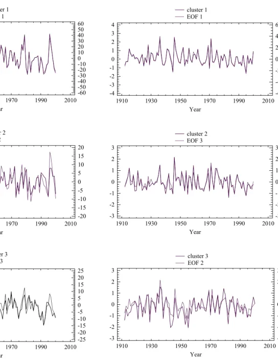
Fig. 10. Temporal evolution of the centroid series (left axis, contin-uous line) and principal component series (right axis, dashed line) for the period 1912–2000, corresponding to each cluster/EOF for winter.
influence of local convective storms in September (Sumner et al., 2001).
As a main result, both methods establish a similar region-alization, with slight differences mainly in summer and au-tumn, when local mechanisms (convective rainfall) are more important than large-scale rainfall forcings.
4.2 Temporal patterns
The centroid series in CA is analogous to the principal com-ponent series in PCA. While the centroid series consists of the simple average of the individual elements belonging to
33 Year cluster 1 EOF 1 1910 1930 1950 1970 1990 2010 -4 -3 -2 -1 0 1 2 3 4 -60 -40 -20 0 20 40 60 Year cluster 2 EOF 3 1910 1930 1950 1970 1990 2010 -3 -2 -1 0 1 2 3 -30 -20 -10 0 10 20 30 Year cluster 3 EOF 2 1910 1930 1950 1970 1990 2010 -3 -2 -1 0 1 2 3 -30 -20 -10 0 10 20 30 Figure 11
Fig. 11. As Fig. 10, for spring.
the cluster, the principal component is the result of a linear combination of the original data. To compare both meth-ods, correlation coefficients between centroid series and the principal components associated with the EOFs that show a regionalization similar to that of the CA have been calcu-lated. Results are shown in Table 3. All the coefficients were significant at the 99% confidence level. Note that the best results correspond to cluster 1 and EOF 1 for winter, spring and autumn, an area mainly affected by fluctuations in west-ern circulation, and in particular, by fluctuations of the North Atlantic Oscillation. Figures 10 to 13 represent the time evo-lution of the centroid and principal component series for each season of the year. Scale differences are due to the fact that in CA we obtain the average from the members of the cluster,
1446 D. Mu˜noz-D´ıaz and F. S. Rodrigo: Spatio-temporal patterns of seasonal rainfall in Spain (1912–2000) 34 Year cluster 1 EOF 3 1910 1930 1950 1970 1990 2010 -3 -2 -1 0 1 2 3 -20 -15 -10 -5 0 5 10 15 20 Year cluster 2 EOF 1 1910 1930 1950 1970 1990 2010 -4 -3 -2 -1 0 1 2 3 4 -25 -20 -15 -10 -5 0 5 10 15 20 25 Year cluster 3 EOF 1 1910 1930 1950 1970 1990 2010 -3 -2 -1 0 1 2 3 -25 -20 -15 -10 -5 0 5 10 15 20 25 Year cluster 4 EOF 2 1910 1930 1950 1970 1990 2010 -4 -3 -2 -1 0 1 2 3 4 -30 -20 -10 0 10 20 30 Figure 12
Fig. 12. As Fig. 10, for summer.
while in PCA each of the principal component is a sort of weighted average of the original data. As a result, the range of centroid series is less. However, the main result is the great similarity of series, showing identical distribution of positive and negative anomalies.
In general terms, all the time series show a fluctuating be-haviour, with alternating dry and wet periods. With regards to the winter series (Fig. 10), important dry periods can be detected, for, example, around 1920 for the three regions, or around 1990 for the western (C1, EOF1) and northern (C3, EOF3) regions, and noticeably wet periods, for instance,
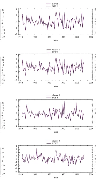
35 Year cluster 1 EOF 1 1910 1930 1950 1970 1990 2010 -2 -1 0 1 2 -25 -20 -15 -10 -5 0 5 10 15 20 25 Year cluster 2 EOF 1 1910 1930 1950 1970 1990 2010 -3 -2 -1 0 1 2 3 -25 -20 -15 -10 -5 0 5 10 15 20 25 Year cluster 3 EOF 3 1910 1930 1950 1970 1990 2010 -2 -1 0 1 2 -15 -10 -5 0 5 10 15 Year cluster 4 EOF 2 1910 1930 1950 1970 1990 2010 -4 -3 -2 -1 0 1 2 3 4 -20 -15 -10 -5 0 5 10 15 20 Figure 13
Fig. 13. As Fig. 10, for autumn.
around 1960 for the Mediterranean region (C2, EOF2). In spring (Fig. 11), a prolonged dry period began around 1970 for the western (C1, EOF1) and Mediterranean (C2, EOF3) regions, and another dry period is detected from approxi-mately 1935 to 1955 for northern region (C3, EOF2). Wet peaks can be seen around 1945 for western (C1, EOF1) and Mediterranean (C2, EOF3) areas. In summer (Fig. 12), a season normally dry, wet peaks are detected around 1930 for northern (C2, EOF1, and C3, EOF1) and southwest (C4, EOF2) areas, and around 1975 for Mediterranean regions (C1, EOF3 and C2, EOF1). Finally, in autumn (Fig. 13) wet
peaks can be seen from 1960 to 1970, and a dry period is detected from 1970 to 1995 for the four regions. The pre-dominance of dry conditions in Spain during the last decades of the century has been related to the predominance of the positive phase of the North Atlantic Oscillation during this period (Hurrell et al., 2003).
5 Conclusions
Unfortunately, Portuguese data were not available for this work. However, other analysis (e.g. Goodess and Jones, 2002; Rocha, 1999) covering the whole Iberian Peninsula, include Portugal in the western area. The inclusion of Por-tuguese data, therefore, would enlarge the regions estab-lished in this work, that is, cluster 1 for autumn, winter, and spring, and cluster 4 for summer.
PCA method is an alternative to traditional CA tools to obtain homogeneous groups. In PCA, variables are assigned to groups according to their loading factor values. PCA re-gions are “fuzzy”, that is, the main difference lies in the fact that PCA solutions may be overlapping, with some variables may be included in more than a single group (Gong and Richman, 1995). The analyses presented in Sect. 4.1 indi-cate that there are three regions (clusters) of seasonal rainfall over the Iberian Peninsula in winter and spring: the west-ern area of the Peninsula, the eastwest-ern Mediterranean Coast, and the northern zone. Four clusters have been obtained in summer and autumn, when local and convective mech-anisms are more important in rainfall generation. On the other hand, PCA results are very similar, with the first EOFs corresponding to the regions established by CA, mainly in winter and spring. These broad regionalizations are sup-ported by other studies (Rod´o et al., 1997; Esteban-Parra et al., 1998; Rodr´ıguez-Puebla et al., 1998; Mart´ın-Vide and G´omez, 1999; Serrano et al., 1999; Goodess and Jones, 2002). They are based on the analysis of 32 stations. The Iberian topography and other geographical factors are re-sponsible for spatial heterogeneity at the sub-regional scale (Romero et al., 1999). A certain annual cycle is detected if the spatial patterns of the different seasons are compared.
While CA includes the complete variance of original data, PCA allows one to distinguish between “signal” and “noise”. Noise in original data is excluded if the dimensionality re-duction stage of the PCA is successful. Conversely, tradi-tional CA includes the full original raw variance information. In this sense, PCA is a technique more powerful than CA. However, the use of standardized anomalies as input data in CA allows one to obtain analogous time series to describe this variability. Although the series obtained are fluctuat-ing, with alternating dry and wet peaks, some features can be noted, mainly the predominance of dry conditions in the last decades of the century, coinciding with the predominance of the positive phase of the North Atlantic Oscillation during this period (Hurrell et al., 2003). The analysis of the influ-ence of the North Atlantic Oscillation on these series will be the object of a work now in preparation.
The fact that CA does not restrict the input database to particular statistical distributions (Gaussian) and the coinci-dences with the results of applying PCA allow one to affirm that, at least in a first approach, CA is a suitable tool to de-scribe the variability of rainfall in the study region.
Acknowledgements. This work has been sponsored by the Spanish Science and Technology Ministry under the REN2001-3923-C02-02/CLI project.
Topical Editor O. Boucher thanks a referee for his help in eval-uating this paper.
References
Ahmed, B. Y. M.: Climatic classification of Saudi Arabia: an appli-cation of factor-cluster analysis, GeoJournal, 41.1, 69–84, 1997. Almarza, C., L´opez, J. A., and Flores, C.: Homogeneidad y vari-abilidad de los registros hist´oricos de precipitaci´on de Espa˜na, Instituto Nacional de Meteorolog´ıa, Madrid, 1996.
Anderberg, M. R.: Cluster Analysis for Applications, Academic Press, California, 1973.
Blashfield, R. K.: Mixture model tests of cluster analysis: Accuracy of four agglomerative hierarchical methods, Psychol. Bull., 83, 377–388, 1976.
DeGaetano, A. T.: Spatial grouping of United States climates sta-tions using a hybrid clustering approach, Int. J. Climatol., 21, 791–807, 2001.
DeGaetano, A. T. and Shulman, M. D.: A climatic classification of plant hardiness in the United States and Canada, Agrc. For. Meteorol., 51, 333–351, 1990.
Esteban-Parra, M. J., Rodrigo, F. S., and Castro-D´ıez, Y.: Spatial and temporal patterns of precipitation in Spain for the period 1880–1992, Int. J. Climatol., 18, 1557–1574, 1998.
Gong, X. and Richman, M. B.: On the application of cluster anal-ysis to growing season precipitation data in North America East of the Rockies, J. Clim., 8, 897–931, 1995.
Goodess, C. and Jones, P. D.: Links between circulation and changes in the characteristics of Iberian rainfall, Int. J. Clima-tol., 22, 1593–1615, 2002.
Halkidi, M., Batistakis, Y., and Vazirgiannis, M.: On clustering val-idation techniques, Journal of Intelligent Information Systems, 17:2/3, 107–145, 2001.
Hulme, M. and Sheard, N.: Escenarios de cambio clim´atico para la Peninsula Ib´erica, Climatic Research Unit, Norwich, 1999. Hurrell, J. W., Kushnir, Y., Ottersen, G., and Visbeck, M.: An
Overview of the North Atlantic Oscillation, edited by J. W. Hur-rell, Y. Kushnir, G. Ottersen, and M. Visbeck, The North Atlantic Oscillation, Climatic Significance and Environmental Impact, 1– 35, American Geophysical Union, Washington DC, 2003. Kaufman, L. and Rousseuw, P. J.: Finding Groups in Data: An
Introduction to Cluster Analysis, Wiley, New York, 1990. Lana, X. and Burgue˜no, A.: Some statistical characteristics of
monthly and annual pluviometric irregularity for the Spanish Mediterranean Coast, Theor. App. Clim., 65, 79–97, 2000. Mart´ın-Vide, J., and G´omez, L.: Regionalization of peninsular
Spain base don the length of dry spells, Int. J. Climatol., 19, 537– 555, 1999.
Mart´ınez Arias, R.: El an´alisis multivariante en la investigaci´on cient´ıfica, Editorial La Muralla, S. A., Madrid, 1999.
O’Lenic, E. A. and Livezey, R. E.: Practical considerations in the use of rotated principal component analysis (RPCA) in
diagnos-1448 D. Mu˜noz-D´ıaz and F. S. Rodrigo: Spatio-temporal patterns of seasonal rainfall in Spain (1912–2000) tic studies of upper-air height fields, Mon. Weather Rev., 116,
1682–1689, 1998.
Ojo, S. O. and Afiesimama, E. A.: Uso de promedios de periodos de referencia para examinar anomal´ıas del clima, Bolet´ın de la Organizaci´on Meteorol´ogica Mundial, 49, 288–291, 2000. On-Kim, J.: Factor analysis, edited by Nie, N. H., Jenkins, J. G.,
Steinbrenner, K., Bent, D. H., Statistical package for social sci-ences (spcc), 468–514, McGraw-Hill, New York, 1970. Preisendorfer, R. W.: Principal Component Analysis in
Meteorol-ogy and Oceanography, edited by Mobley, C. D., Elsevier, Ams-terdam, 1988.
Ramos, M. C.: Divisive and hierarchical clustering techniques to analyse variability of rainfall distribution patterns in a Mediter-ranean region, Atmos. Res., 57, 123–138, 2001.
Rocha, A.: Low-frequency variability of seasonal rainfall over the Iberian Peninsula and ENSO, Int. J. Climatol., 19, 889–901, 1999.
Rod´o, X., Baert, E., and Comin, F. A.: Variations in seasonal rain-fall in southern Europe during the present century: relationships with the North Atlantic Oscillation and the El Ni˜no-Southern Os-cillation, Clim. Dyn., 19, 275–284, 1997.
Rodr´ıguez-Puebla, C., Encinas, A. H., Nieto, S., and Gardenia, J.: Spatial and temporal patterns of annual precipitation variability over the Iberian Peninsula, Int. J. Climatol., 18, 299–316, 1998.
Rogers, J. C.: Patterns of low-frequency monthly sea level pres-sure variability (1899–1986) and associated wave cyclone fre-quencies, J. Clim., 3, 1364–1379, 1990.
Rogers, J. C. and McHugh, M. J.: On the separability of the North Atlantic oscillation and Artic oscillation, Clim. Dyn., 19, 599– 608, 2002.
Romero, R., Sumner, G., Ramis, C., and Genoves, A.: A classifica-tion of the atmospheric circulaclassifica-tion patterns producing significant daily rainfall in the Spanish Mediterranean area, Int. J. Climatol., 19, 765–785, 1999.
Serano, A., Garc´ıa, J. A., Mateos, V. L., Cancillo, M. L., and Gar-rido, J.: Monthly modes of variation of precipitation over the Iberian Peninsula, J. Clim., 12, 2894–2919, 1999.
Sumner, G., Homar, V., and Ramis, C.: Precipitation seasonality in eastern and southern coastal Spain, Int. J. Climatol., 21, 219– 247, 2001.
Trigo, R. M. and Palutikof, J. P.: Precipitation scenarios over Iberia: a comparison between direct GCM output and different down-scaling techniques, J. Clim., 14, 4422–4446, 2001.
Von Storch, H. and Zwiers, F. W.: Statistical analysis in climate research, Cambrigde University Press, Cambridge, 1999. Ward, J. H.: Hierarchical grouping to optimise an objective
func-tion, J. Amer. Stat. Assoc., 58, 236–244, 1963.
Wilks, D. S.: Statistical Methods in the Atmospheric Sciences, Aca-demic Press, California, 1995.