Abstract— We derive the statistics for the multilook intensity ratio for a multilayered medium bounded by randomly rough surfaces. Calculations are carried out in the context of the first-order small perturbation method and assume slightly rough surfaces of infinite extent and centered Gaussian height distributions. We show that the probability distributions for the co-polar and cross-polarized intensity ratios for n-look data are functions of three parameters and that the mean exists for n1
and the variance for n2. The obtained theoretical expressions are verified by comparison with Monte-Carlo results.
Index Terms— Multilook intensity ratio, layered rough surfaces, scattering amplitudes, small perturbation method.
I. INTRODUCTION
CATTERING of electromagnetic waves from rough surfaces or multilayered media bounded by randomly rough interfaces is encountered in a large number of physical problems, for remote sensing, civil engineering, geophysics or optics applications. The Small Perturbation Method (SPM) is often used for the analysis of these scattering phenomena. This model is based on Taylor series of the scattering amplitudes and of the boundary value problem and gives closed-form expressions for the coherent and incoherent scattered intensities [1]-[9]. The rigorous methods associated with numerical techniques have the advantage that they do not rely on simplifying approximations [10-15]. But, they require the computation of solutions for a large number of realizations of rough surfaces or multilayered media. Within its domain of validity [6]-|8], the SPM allows a fast analysis unlike to the high computational burden of numerical solutions.
Polarimetric synthetic aperture radar has proven to be an efficient tool for geophysical remote sensing [16]. The co- and cross-polarized intensity ratios are widely used indicators for the analysis of polarimetric data [17]. To reduce statistical variations, polarimetric radars use the multilook processing by averaging spatially the backscattered intensities. The statistics of single-look and multilook polarimetric SAR data have been
Manuscript received October 02, 2019.
Richard Dusséaux is with the Laboratoire Atmosphères, Milieux, Observations Spatiales (LATMOS), Université de Versailles Saint-Quentin-en-Yvelines (UVSQ/Paris-Saclay), 11 boulevard d'Alembert, 78280 Guyancourt, France. (e-mail: richard.dusseaux@ latmos.ipsl.fr).
Saddek Afifi is with the Electronics Department, Badji Mokhtar – Annaba University, BP 12, 23000, Annaba, Algeria..(e-mail: [email protected]).
investigated under the hypothesis of multivariate Gaussian and K-distribution models for the underlying complex scattering amplitudes [18]-[21]. The derivations presented in [18]-[21] are relevant but the connection with an electromagnetic model is not made [22]-[24].
In [25], we derive the closed-form expression for the probability distribution for the scattered intensity ratio for a stratified medium under a monochromatic plane wave illumination. The scattered intensities are derived from the first-order small perturbation method and we assumed slightly rough interfaces of infinite extent and centered Gaussian height distributions. For single-look signatures, the co- and cross-polarized intensity ratios follow heavy-tailed distributions which don’t have finite mean and variance. In [26], we showed that the statistics of the co- and cross-polarized intensity ratios allow differentiating a stratification air/clayey soil/rock with or without snow cover. In [27], we derive the statistics for the Normalized Difference Polarization Index (NDPI) which is defined as the ratio of the difference between two intensities under different polarizations on the sum of these two intensities. The NDPI therefore takes values between – 1 and 1. Contrary to the intensity ratio, the first and second order statistical moment values of this discriminator are finite.
In the present paper, we are interested in the statistical properties of the co- and cross-polarized intensity ratios but for multilook configurations. We derive the theoretical expressions for the probability density function (PDF) and the cumulative distribution function (CDF) for a stratified medium bounded by random slightly rough interfaces under a plane wave illumination. The scattered intensities are given by the first-order SPM [3]-[4]. For electromagnetic signatures based on more than two looks, we show that the probability distribution has finite mean and variance. To our knowledge, it is the first time that the analytical expressions for the mean and variance and the CDF are found.
This paper is organized as follows. Section II is dedicated to the statistical properties of the stratified medium. Section III is devoted to the analytical expressions derived from the first-order SPM for the scattering amplitudes and the scattered intensities. In section IV and appendix, we derive closed-form expressions for the PDF and CDF and for the mean and variance. In Section V, the theory is verified by comparison with Monte-Carlo results.
Multilook Intensity Ratio Distribution for 3D
Layered Structures with Slightly Rough
Interfaces
Richard Dusséaux and Saddek Afifi
II. ANALYZED STRUCTURE
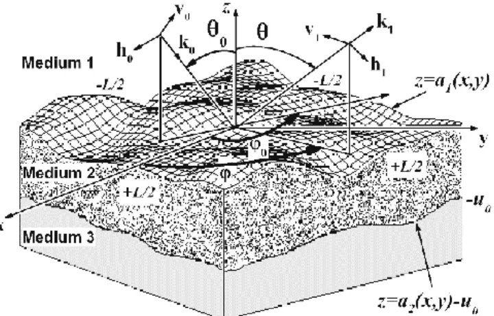
As shown in Fig. 1, the structure we consider is a stack of two surfaces separating three media. The rough surfaces are randomly deformed over an area L L . The quantity u0 designates the layer average thickness. The two boundaries are located at the height za x y1( , ) and za x y2( , )u0. They are realizations of second order stationary, centered Gaussian stochastic processes with Gaussian spectrum ˆ ( , )Rii :
2 2 2 2 2 ˆ ( , ) exp 4 xi yi ii i xi yi l l R l l (1)
There are two distinct correlation lengths, lxi and l . The i-th yi interface is isotropic if lxi lyi and anisotropic if lxi lyi.
The rms-heights i are small numbers compared to the incident wavelength and the gradients of the surface height functions a x y are much smaller than 1 so that the i( , ) perturbation method may be used to study wave scattering [6]-[8].
The cross-spectrum Rˆ ( , )12 is given in the following form:
12 1 2 1 2 1 2 2 2 2 2 1 2 2 1 2 2 ˆ ( , ) ( ) ( ) exp 8 8 x x y y y y x x R q l l l l l l l l (2)
The coefficient q is a mixing parameter with q1 [3], [26]. If 0
q , both rough interfaces are uncorrelated, otherwise, they are fully or partially correlated.
A monochromatic h- or v-polarized plane wave of wavelength impinges on the structure. The incident direction is defined by the wave vector k and the angles 0 0 and 0. The structure is composed of three different regions characterized by an isotropic and homogeneous permittivity. The top and bottom regions are half-spaces. The permeability of all regions is assumed to be 0.
III. SCATTERED INTENSITY AS A RANDOM PROCESS For an observation direction defined by the angles and (see Fig. 1), the first-order amplitudes of the co- and cross-polarized contributions of the field scattered in the upper region are derived from the SPM as follows [3]:
(1) 1,( ) 1,( ) 1 0 0 2,( ) 2 0 0 ˆ ( , ) ( , ) ( , ) ˆ ( , ) ( , ) ba ba ba A K a K a (3)
with ksin cos , ksin sin , 0 ksin0cos0,
0 ksin 0sin 0
and k 2 / . The subscript (a) gives the impinging plane wave polarization (h or v) and the subscript (b), the scattered wave polarization (h or v), respectively. The function aˆ ( , )i is the Fourier transform of the functiona x yi( , ). The quantities Ki ba,( )( , ) are the first-order SPM kernels [3].
The normalized scattered intensity I(ba) is defined as the power scattered per unit of solid angle divided by the incident power. In the direction (,), the first-order perturbation theory gives I(ba) as follows [3],
2 2 (1) 0 ( ) 2 ( ) cos ( , ) ( , ) cos ba ba I A (4) where (1) (1) (ba)( , ) (ba)( , ) /
A A L. The scattered intensity
(ba)( , )
I depends on rough boundary height profile realizations and for a given direction, it is a random variable. When L , the mean of I(ba)( , ) is given by,
( ) 2 2 2 * 0 ,( ) ,( ) 0 0 2 1 1 ( , ) cos ˆ Re[ ( , )] cos ba i ba j ba ij i j I K K R
(5)where the brackets denote a statistical average over the ensemble of realizations of I(ba)( , ) .
IV. MULTILOOK INTENSITY RATIO STATISTICS A. Scattering amplitudes as complex random variables
Let I(ba)( , ) and I( ' ')b a ( , ) be the (b)- and (b’)-polarized contributions of the scattered intensity under the (a)- and (a’)-polarized incident waves, respectively. In a first stage, we determine the joint PDF
(ba),( ' ')b a ( , ) I I
p w w for the single-look data I(ba)( , ) and I( ' ')b a ( , ) . In a second stage, we derive from the closed-form formula of
(ba),( ' ')b a ( , ) I I
p w w the joint probability law for the multilook intensities and finally, the probability law for the multilook intensity ratios.
Let R(ba)( , ) and J(ba)( , ) be the real and imaginary
parts of the scattering amplitude A((1)ba)( , ) and let
( ' ')b a ( , )
R and J( ' ')b a ( , ) be the real and imaginary ones of
(1) ( ' ')b a ( , )
A , respectively. We assume that the height distributions of both interfaces are centered and Gaussian. Fig. 1. Structure with two nonparallel interfaces
Since any linear operator transforms a Gaussian process into another Gaussian process, we deduce that the first-order scattering amplitudes given by (3) are Gaussian processes and that the joint PDF of the random variables R(ba)( , ) ,
(ba)( , )
J , R( ' ')b a ( , ) and J( ' ')b a ( , ) is a four-dimensional Gaussian function. So, it is necessary to determine the covariance matrix characterizing this Gaussian law. Insofar as the rough surface height distributions are centered, the random variables R(ba)( , ) , J(ba)( , ) , R( ' ')b a ( , ) and J( ' ')b a ( , ) are also centered. We showed in [3] that the random variables
(ba)( , )
R and J(ba)( , ) (respectively, R( ' ')b a ( , ) and
( ' ')b a ( , )
J ) are asymptotically uncorrelated (when L ) with equal variances 2
ba R
. The random variables R(ba)( , ) and R( ' ')b a ( , ) are correlated with a covariance
R Rba b a' ' andlikewise, the random variables R(ba)( , ) and J( ' ')b a ( , ) are also correlated with a covariance
' '
ba b a R J
. These statistical moments are defined as follows [3], [25]:2 2 2 * ,( ) ,( ) 0 0 1 1 1 ˆ Re[ ( , )] 2 ba R i ba j ba ij i j K K R
(6) ' ' 2 2 * ,( ) ,( ' ') 0 0 1 1 1 ˆ Re[ ( , )] 2 ba b a R R i ba j b a ij i j K K R
(7) ' ' 2 2 * ,( ) ,( ' ') 0 0 1 1 1 ˆ Im[ ( , )] 2 ba b a R J i ba j b a ij i j K K R
(8)We find from (5) and (6) that:
2 2 0 ( ) 2 cos ( , ) 2 cos ba ba R I (9)
B. Probability density function of the multilook intensity ratio By using polar coordinates, we derive from the joint PDF of
(ba)
R , J(ba), R( ' ')b a and J( ' ')b a the 4D-PDF of modulus M(ba) and M( ' ')b a and phases (ba) and ( ' ')b a of scattering amplitudes A((1)ba)( , ) and A( ' ')(1)b a ( , ) . By integrating over the phases, we obtain the joint PDF
(ba), ( ' ')b a ( , )
M M
p m m of the modulus M(ba) and M( ' ')b a and we find from
(ba), ( ' ')b a ( , )
M M
p m m the joint probability law
(ba),( ' ')b a ( , ) I I
p w w for the intensities I(ba) and I( ' ')b a [25],
( ) ( ' ') 2 0 0 0 , 2 2 0 0 0 0 2 ( , ) exp ( ) 1 1 2 1 ba b a I I p p w w w p w r r r p ww I r (10) where ' ' 2 ( ) 0 2 ( ' ') ( , ) ( , ) ba b a R ba R b a I p I (11) and 2 0 0 2 2 cos 2 cos ba R (12)
The function I0 denotes the zeroth-order modified Bessel function. The quantity r is the modulus of the correlation coefficient between the two complex random variables
(1) (ba)( , ) A and (1) ( ' ')b a ( , ) A with 0 r 1: ' ' ' ' ' ' 2 2 2 2 ba b a ba b a ba b a R R R I R R r (13)
The n-look averaged intensity is defined as follows:
( ) ( ), 1 1 n ba ba i i I I n
(14) We assume that the n-look intensities are means of n independent identically distributed random variables. Because the n-look intensities are identically distributed, all the random variables I(ba i), /n (1 i n) follows the same probability law0 (ba), 0 ( ' ')b a ( 0 , 0 ' ') I I ba b a p w w with:
0 ( ), 0 ( ' ') ( ) ( ' ') ( ) ( ' ') ' ' 0 0 ' ' , 2 , ' ' , , , ba b a ba b a ba b a ba b a I I ba b a I I n n I I ba b a w w p w w p n n n p nw nw (15)Because the n-look intensities are independent random variables, the joint probability law
(ba),( ' ')b a ( ba, b a' ') I I p w w is found by convolving 0 (ba), 0 ( ' ')b a ( 0 , 0 ' ') I I ba b a p w w with itself 1
n times [28, chap. 5]. For determining this joint PDF, we also use, as in [19], the properties of the two-dimensional Laplace transform of
0 (ba), 0 ( ' ')b a
(
0,
0 ' ')
I I ba b ap
w
w
. Themathematical derivation is included in the appendix and gives the following analytical expression,
( ) ( ' ') 1 1 ( 1)/2 0 0 0 1 2 , 0 0 0 1 0 2 2 ( ) ( , ') (1 ) ( 1)! 2 exp ( ) 1 1 ba b a n n n n I I n p n p ww p w w r r n n rn w p w I p ww r r (16)
where In1 is the (n1)-th order modified Bessel function. Let Vn ba b a,( , ' ') I(ba)/I( ' ')b a be the n-look intensity ratio. Finally, we obtain the PDF for the ratio Vn ba b a,( , ' ')as follows:
,( ,' ')( ) 0 ( ),( ' ')( , )
n ba b a ba b a
V I I
p v
w p vw w dw (17) By substituting (16) into (17), we find:,( ' ') 1 1 ( 1)/2 ( 1)/2 0 0 , 1 2 0 0 0 1 2 0 2 0 ( ) (1 ) ( 1)! 2 exp ( ) 1 1 n ba b a n n n n n V n n n v p p v w r r n rn n I p vw v p w dw r r
(18)By using the following relation found in the Laplace transform table [29, p. 73, Eq. 6],
1 1 2 2 1/2 0 2 ( 1 / 2) ( ) exp ( ) n n n n n n a s x I ax sx dx s a
(19)where the letter
designates the Gamma function, we get the probability distribution,( ,' ')( )
n ba b a V
p v for the multilook intensity ratio: ,( ' ') 2 1 0 0 , 2 2 2 1/2 0 0 (1 ) ( ) (2 ) ( ) ( ) ( ) 2 (1 2 ) n ba b a n n n V n r p v v p n p v n n v vp r p (20)
The PDF only depends on the three parameters n, r and
0
p . For n1, we get the PDF for the single-look intensity ratio. It’s a heavy-tailed distribution with infinite mean and variance.
The closed-form expression (20) has been established in [19] and [20]. The derivation begins with a multivariate Gaussian model for the underlying complex scattering amplitudes. But, our approach is not based on the a priori assumption that the complex scattering amplitudes follows a multivariate Gaussian distribution. For slightly rough interfaces with Gaussian height distributions, we establish this property in the context of the first-order SPM.
C. Cumulative density function of the multilook intensity ratio We find from (20) the recurrence relation between
,( ,' ')( ) n ba b a V p v and 1,( ,' ')( ) n ba b a V p v : 1,( ' ') ,( ' ') 2 2 0 0 , 2 0 , 2 (1 2 ) ( ) 2 1 2(1 ) ( ) n ba b a n ba b a V V p v p r p v v n r p p v n (21)
By integration, we find from (21):
1,( ' ') 1,( ' ') 1,( ' ') ,( ' ') 2 0 , , 0 , 2 2 0 0 , 0 2 (1 2 ) ( ) ( ) ( ) 2 1 2(1 ) ( ) n ba b a n ba b a n ba b a n ba b a v V V v V V p r F v xp x dx p x n p dx r p F v x n
(22)where the function
,( ,' ')
( )
n ba b a V
F
v
designates the CDF for the n-look intensity ratio. We write the (n+1)-n-look PDF as follows:1,( ' ') 0 , 1 1 1/ 2 ( ) ( ) ( ) n ba b a n V n n v v p p v q R v (23) where 2 ( ) R v cv bva with, 2 0 2 0 2 (1 2 ) 1 a p b p r c (24) and, 2 1 1 1 0 (2 2) (1 ) ( 1) ( 1) n n n n q r p n n (25)
In accordance with the following recursion formula [30, Eq. (2.263), p.95] with m2n, 1 , 1/2 1, 2, (2 2 1) ( 2 ) 2( 2 ) ( 1) ( 2 ) m m n n m n m n x m n b K K m n cR m n c m a K m n c (26) where , 1/2 m m n n x K dx R
(27) we find from (23), 1( ) 1 1, 1 1 0 , 1 n n n n n n n F v qK q p K (28) and we also establish that,
1 1 0 0 1 2, 1 0 1, 1 , 1 0 1, 1 ( ) ( ) v v n n n n n n n n n n n p x xp x dx a dx x q K p K aK ap K
(29)By substituting (29) into (22) and using the relation (26), after some algebraic manipulations, we obtain a mathematical recurrence formula for the CDF:
1,( ' ') ,( ' ') 0 ,
( )
,( )
n ba b a n ba b a n V V nv
p
v
F
v
F
v
q
R
R
(30)Finally, we obtain from (30) the analytical expression of
,( ,' ')( ) n ba b a V F v : ,( ' ') 1,( ' ') 0 , , 2 2 2 0 0 2 1 0 2 2 2 1 0 0 ( ) ( ) 2 (1 2 ) (1 ) (2 ) ( ) ( ) 2 (1 2 ) n ba b a ba b a V V m n m v p F v F v v vp r p r p v m m m v vp r p
(31)where the function
1,(ba b a,' ')( )
V
F v is the CDF for a single-look intensity ratio. We established in [25] that
1,( ' ') 0 , 2 2 2 0 0 1 ( ) 2 2 2 (1 2 ) ba b a V v p F v v vp r p (32)
This is new compared to previous works on the n-look intensity ratio statistics. We find from (31) that for any n,
0 1 0
( ) ( ) 0.5
n
F p F p . As a result, the median of Vn ba b a,( , ' ') is
0
p for any value of n.
D. Mean and variance of the multilook intensity ratio
Using the recurrence formula (26), we show that the mean
,( , ' ') n ba b a V of Vn ba b a,( , ' ') exists ifn1 with, 2 0 ,( , ' ') ( ) ( 1) n ba b a n r p V n (33)
and that the variance
,( , ' ') 2
n ba b a V
,( , ' ' 2 2 0 ) 2 2 2 2 ( 1) ( 2) (2 1) 4( 1)(1 ) (2 ) n ba b a V p n n n n r n r n n r (34)The mean Vn ba b a,( , ' ') and the standard deviation
,( , ' ')
n ba b a V
increase linearly with p0. The limit of the mean is p0 as n tends to infinity and, the limit of the variance is zero. When n goes to infinity, the intensity ratio value is no longer random.
For uncorrelated scattered amplitudes (1) (ba)
A and (1) ( ' ')b a A , 0
r . For this case, the multilook intensity ratio follows a Fisher distribution for which the closed-form expressions for the mean and variance are well known [31]. To the best of our knowledge, it is the first time that the analytical expressions for the mean and variance for correlated scattered amplitudes are found.
V. NUMERICAL RESULTS
We consider a two-layer rough ground. The wavelength
is equal to 24 cm. The relative dielectric constants of the ground layers are r2 4.66-0.29j andr3 8.750.85j at 1.25 GHz [32]. The rms-heights are 10.5 cm and2 0.4 cm
for the upper and lower surfaces, respectively. A 5cm-thickness (u in Fig. 1) is assumed for the middle layer 0 [33]. The Gaussian spectrum of the upper interface is anisotropic with the correlation lengths lx15 cm and
1 4 cm
y
l . The lower interface spectrum is isotropic with
2 2 6 cm
x y
l l . Both random surfaces are partially correlated with a correlation coefficient 12 equal to 0.2. The incident wave vector angles 0 and 0 are equal to 30° and 0°.
Fig. 2 shows the PDFs of the co-polarized intensity ratio
,( , )
n hh vv
V in the backscattering direction. The theoretical probability law obtained for surfaces of infinite extent is given by (20). The histograms are estimated over results associated with 213 surface realizations where L20
[26]. The probability law is representative of the values which the intensity ratio can take and does not lose some details as for the statistical averages. The agreement between the theoretical probability law with the histogram obtained from Monte-Carlo simulations is very good for each value of n and validates the theory for the co-polarized intensity ratio in the backscattering direction.Given the simulation parameter values, the correlation coefficient ris equal to 0.994 and therefore, the co-polarized scattering amplitudes A((1)hh) and
(1) (vv)
A are strongly correlated. The parameter p is equal to 0.542, which means that 0
(hh) 0.542 (vv)
I I
. As shown by Fig. 2, as the number of looks increases, the PDF curve becomes narrower and concentrated near p because multilook processing reduces 0 the statistical variation and this causes an increase of the maximum value of the PDF.
Fig. 3 shows the theoretical CDF and the CDF estimated from the set of realizations of the co-polarized scattered intensities. For each value of n, the two curves are superimposed. As the number of looks increases, the CDF becomes a staircase function about the value p because the 0 reduction of the statistical variation by the multilook processing.
Fig.4 compares the values of the theoretical mean and standard deviation of Vn hh vv,( , )( 30 , 0 ) with the values estimated over Monte-Carlo simulations versus the number of looks. The comparison is conclusive. These curves show that the mean Vn hh vv,( , ) quickly converges towards the median p and for large values of 0 n, the standard Fig. 2. Theoretical PDF of random variable Vn hh vv,( , )( 30 , 0 ) and
normalized histogram for n=1, 2, 4 and 8.
Fig. 3. Theoretical CDF of random variable Vn hh vv,( , )( 30 , 0 ) and
CDF estimated from Monte-Carlo simulations for n=1, 2, 4 and 8.
Fig. 4. Values of theoretical means and standard deviation of
,( , )( 30 , 0 )
n hh vv
V and values estimated over Monte-Carlo simulations versus number of looks
deviation
,( , )
n hh vv V
decreases in 1 / n .
In the plane perpendicular to the incidence plane, there is a depolarization and we established in the context of the first-order perturbation theory that the cross-polarized intensity ratio is only defined for a (v)-polarized impinging plane wave [34]. Fig. 5 shows the theoretical PDF of Vn hv vv,( , )( 30 ,90 ) and the associated histogram for four values of n. Given simulation parameter values, the correlation coefficient r is equal to 0.872 and therefore, the co-polarized scattering amplitude A((1)vv) and the cross-polarized amplitude A((1)hv) are strongly correlated. The parameter p0 is equal to 11.2 and
(hv) 11.2 (vv)
I I
. As a result, for this medium under consideration, the depolarization is strong within the transverse plane. At n1, the random variable V1,(hv vv, ) follows a heavy-tailed law and has a large amount of skewness. As
n
increases, the PDF starts to become symmetrical about v p0 so that the ratio mean approaches p and the maximum value increases. 0 As previously mentioned, the histograms are estimated from 213 realizations over areas of 2400 . We find a very good agreement between the histograms and the corresponding theoretical probability laws for the four values of the number of looks.
Fig. 6 shows the theoretical CDF and the CDF estimated from Monte-Carlo simulation data. For each value of n, the two curves are superimposed and this comparison validates the analytical formulation for the CDF for the cross-polarized ratio. At n1, the distribution has a heavy tail and as a result, the CDF converges very slowly towards 1 as the ratio tends to positive infinity. As n increases, the convergence is faster.
Fig.7 gives the values of the theoretical mean and standard deviation for the random variable Vn hv vv,( , )( 30 ,90 ) and the values estimated over Monte-Carlo simulations versus the number of looks. As previously in the backscattered direction, the mean Vn hv vv,( , ) quickly converges towards the median p and for large values of 0 n, the standard deviation
,( , )
n hv vv V
decreases in 1 / n . The comparison is satisfactory and validates the closed-form expressions for the mean and variance for the multilook cross-polarized intensity ratio. For
2
n , there is a slight difference between the estimated and theoretical mean values and for n3, a weak difference for the variance values, respectively. This difference decreases when increasing the area L L .
VI. CONCLUSION
We have derived the theoretical statistics for multilook intensity ratios for 3-D layered structures under a monochromatic plane wave illumination. The derivation begins with a multivariate Gaussian model for the underlying complex scattering amplitudes. In contrast to previous works [19]-[20], our approach is not based on the a priori assumption that the complex scattering amplitudes follow a multivariate Gaussian distribution. For slightly rough interfaces with an infinite extent and centered Gaussian height distributions, we establish this property in the context of the first-order small perturbation method.
Assuming that the n-look intensities are means of n independent identically distributed single look intensities, we obtain a 3-parameter probability distribution and we show that the PDF and CDF only depend on the number of looks n, the correlation coefficient r between the complex scattering amplitudes under study and the ratio p between the 0 associated average single-look intensities. We have shown that the parameter p is the median of the n-look intensity ratio 0 for any value of n and that the mean exists for n1 and the variance for n2, respectively. The mean and the standard deviation of the n-look intensity ratio increase linearly with
0
p . The limit of the mean isp as n tends to infinity and for 0
large values of n, the standard deviation decreases in 1 / n . Fig. 5. Theoretical PDF of random variable Vn hv vv,( , )( 30 ,90 )
and normalized histogram for n=1, 2, 4 and 8.
Fig. 6. Theoretical CDF of random variable Vn hv vv,( , )( 30 ,90 )
and CDF estimated from Monte-Carlo simulations for n=1, 2, 4 and 8.
Fig. 7. Values of theoretical means and standard deviation of
,( , )( 30 , 90 )
n hv vv
V and values estimated over Monte-Carlo simulations versus number of looks.
The obtained formulae are derived from the first-order SPM and they are valid for slightly rough interfaces only.
For a two-layer rough ground, the analytical results were compared with those derived from Monte Carlo simulations. We have assumed an upper interface with an anisotropic Gaussian spectrum and a lower interface with an isotropic one. Both random surfaces are partially correlated. The stratified medium is studied in the backscattering direction and in the transverse plane. The analytical formulas assume rough interfaces with infinite extent. Nevertheless, we have shown by Monte-Carlo simulations that these analytical expressions can be used for surfaces of a few hundred wavelength squared. The agreement between simulated data and theory is observed to be very good for the probability density function, the cumulative density function, the mean and the standard deviation for the co- and cross-polar ratios. We have considered random processes with Gaussian spectra and cross-spectra but the analytical results established in the paper can be used for all random processes with finite memory and for an arbitrary number of interfaces.
APPENDIX
The two-dimensional Laplace Transform (LT2) of
0 (ba), 0 ( ' ')b a 0 , 0 ' ' I I ba b a p w w is defined as follows:
0 ( ), 0 ( ' ') 2 0 ( ), 0 ( ' ') 0 0 ' ' 2 2 0 0 0 0 2 2 0 0 0 0 0 2 ( , ) , exp ( ) 1 1 2 exp ( ) 1 ba b a ba b a I I I I ba b a P s s LT p w w n p n w p w r r rn p ww I sw s w dwdw r
(A1) The determination of 0 (ba), 0 ( ' ')b a ( , ) I IP s s requires two one-dimensional Laplace transforms (LT),
0 ( ), 0 ( ' ') 2 2 0 0 0 0 1 2 2 0 0 1 1 2 0 2 ( , ) exp 1 1 2 ' exp 1 1 ba b a I I n p n p P s s LT w r r rn p ww np LT w I r r (A2)
By using the following representation of the zeroth-order modified Bessel function [29, p. 919, eq. 8.447],
2 0 0 0 0 0 2 2 2 0 2 ' ' 1 1 1 ( !) m m nr p ww rn p ww I r r m
(A3)and after some mathematical calculations, we find:
0 ( ) 0 ( ' ') 2 2 0 0 , 2 0 2 2 2 2 0 0 0 0 1 2 2 2 0 2 1 ( , ) 1 1 exp ' 1 (1 ) 1 ba b a I I n p P s s n r s r n p r n p TL w n r r s r (A4)
The analytical calculation of the last one-dimensional Laplace transform yields: 0 ( ) 0 ( ' ') 2 2 0 0 , 2 2 2 2 0 0 0 0 0 0 0 2 2 2 2 2 ( , ) 1 1 ' ' 1 1 1 (1 ) ba b a I I n p P s s r n p n n p r n p s s s r r r r (A5)
The joint probability law of
(ba),( ' ')b a ( , ) I I p w w is found by convolving
0 (ba), 0 ( ' ')b a 0,
0 ' ' I I ba b ap
w
w
with itself n1 times. The LT2 of the convoluted PDFs is 0 (ba),0 ( ' ')b a ( , )n I I P s s and the joint PDF (ba),( ' ')b a ( , ) I I
p w w is obtained from a 2D inverse Laplace transform ( 1 2 LT ) as follows: ( ) ( ' ') 1 2 , 2 2 0 0 2 2 2 2 0 0 0 0 0 0 0 2 2 2 2 2 ( , ) 1 1 1 1 (1 ) ba b a I I n n p w w LT n p r n p n n p r n p s s s r r r r (A6)
The two-dimensional inverse Laplace transform (A6) becomes with two consecutive one-dimensional inverse Laplace transforms, ( ) ( ' ') 2 2 1 0 0 1 2 , 0 0 2 2 2 2 1 0 0 0 1 2 2 2 1 0 2 1 ( , ) 1 1 1 / 1 (1 ) ( ' ) 1 ba b a n n I I n n p p w w TL r n p s r n r n p TL s np p r r s r (A7) Knowing that
1
1 ( 1)! exp( ) ( ) n n n TL w aw s a (A8)the relationship (A7) becomes:
( ) ( ' ') 2 2 1 0 0 0 2 2 , 2 2 2 1 0 0 0 0 1 2 2 2 0 0 2 ( , ) exp 1 ( 1)! 1 exp / ' 1 (1 ) ( ' ) 1 ba b a n n I I n n p w n p w w w r n r r n p w n p TL s n p r r s r (A9)
By using the following relationship found in the Laplace transform table [29, pp. 245, Eq. 9],
1 ( 1)/ 2 1 1 exp( / ) ( / )n (2 ) n n a s TL w a I aw s (A10)
We find the closed-form formula (16) giving the joint PDF for the multilook intensities I(ba) and I( ' ')b a .
REFERENCES
[1] P. Imperatore, A. Iodice, and D. Riccio, “Electromagnetic wave scattering from layered structures with an arbitrary number of rough interfaces,” IEEE Trans. Geosci. Rem. Sens., vol. 47, no. 4, pp. 1056–1072, Apr. 2009.
[2] A. Tabatabaeenejad and M. Moghaddam, “Bistatic scattering from three-dimensional layered rough surfaces,” IEEE Trans. Geosci. Rem. Sens., vol. 44, no. 8, pp. 2102–2114, Aug. 2006.
[3] S. Afifi and R. Dusséaux, “Scattering by anisotropic rough layered 2D interfaces,” IEEE Trans. Antennas Propag., vol. 60, no. 11, pp. 5315– 5328, Nov. 2012.
[4] S. Afifi, R. Dusséaux, and A. Berrouk, “Electromagnetic scattering from 3D layered structures with randomly rough interfaces: Analysis with the small perturbation method and the small slope approximation,” IEEE Trans. Antennas Propag., vol. 62, no. 10, pp. 5200–5208, Oct. 2014. [5] H. Zamani, A. Tavakoli and M. Dehmollaian, “Scattering from layered
rough surfaces: analytical and numerical investigations,” IEEE Trans. Geosci. Rem. Sensing, vol. 54, no. 6, pp. 3685-3696, Jun. 2016.
[6] J. M. Soto-Crespo, M. Nieto-Vesperinas, and A. T. Friberg, “Scattering from slightly rough random surfaces: A detailed study on the validity of the small perturbation method,” J. Opt. Soc. Amer. A, vol. 7, no. 7, pp. 1185–1201, Jul. 1990.
[7] A. Tabatabaeenejad and M. Moghaddam, “Study of validity region of small perturbation method for two-layer rough surfaces,” IEEE Geosci. Remote Sens. Lett., vol. 7, no. 2, pp. 319–323, Apr. 2010.
[8] P. Imperatore, A. Iodice, M. Pastorino, Nicolas Pinel, “Modelling scattering of electromagnetic waves in layered media: An up-to-date perspective”, Int. Journal of Antennas and Propagation, pp.1-14, 2017. [9] H. Zamani, A. Tavakoli and M. Dehmollaian, "Scattering by a dielectric
sphere buried in a half-space with a slightly rough interface," IEEE Trans. Geosci. Rem. Sensing, vol.66, no.1, pp.347-359, Jan. 2018.
[10] M. El-Shenawee, “Polarimetric scattering from two-layered two dimensional random rough surfaces with and without buried objects,” IEEE Trans. Geosci. Remote Sens., vol. 42, no. 1, Jan. 2001.
[11] N. Déchamps, N. de Beaucoudrey, C. Bourlier, and S. Toutain, “Fast numerical method for electromagnetic scattering by rough layered interfaces: Propagation-inside-layer expansion method,” J. Opt. Soc. Am. A., vol. 23, pp. 359–369, Feb. 2006.
[12] N. Déchamps and C. Bourlier, “Electromagnetic scattering from a rough layer: Propagation-inside-layer expansion method combined to the forward-backward novel spectral acceleration,” IEEE Trans. Antennas. Propag, vol. 55, no. 12, pp. 3576–3586, Dec. 2007.
[13] T. Qiao et al., "Sea Surface radar scattering at L-Band based on numerical solution of Maxwell's equations in 3-D (NMM3D)," IEEE Trans. Geosci. Rem. Sensing, vol.56, no.6, pp.3137-3147, June 2018.
[14] Y. Yang and K. Chen, "Full-polarization bistatic scattering from an inhomogeneous rough surface," IEEE Trans. Geosci. Rem. Sensing, vol.57, no.9, pp.6434-6446, Sept. 2019.
[15] F. Jonard, F. André, N. Pinel, C. Warren, H. Vereecken and S. Lambot, "Modeling of multilayered media Green's functions with rough interfaces," IEEE Trans. Geosci. Rem. Sensing, vol.57, no.10, pp.7671-7681, Oct. 2019.
[16] F.T. Ulaby and C. Elachi, Eds, Radar Polarimetry for Geoscience Applications. Norwood, MA: Attech House, 1990.
[17] P. Mishra and D. Singh, “A statistical-measure-based adaptive land cover classification algorithm by efficient utilization of polarimetric SAR observables,” IEEE Trans. Geosci. Rem. Sens., vol. 52, no. 5, 2889-2900, May 2014.
[18] J.A. Kong, A.A. Swartz, H.A. Yueh, L.M. Novak, and R.T. Shin, “Identification of terrain cover using the optimum polarimetric classifier,” Journal Electromagnetic waves Appl., vol. 8, no. 2, pp.171-194,1987. [19] I.R. Joughin, D.P. Winebrenner and D.B. Percival, “Probability density
functions for multilook polarimetric signatures”, IEEE Trans. Geosci. Rem. Sens., vol. 32, no. 3, pp. 562-574, May 1994.
[20] J.S. Lee, K.W. Hoppel, S. A. Mango, and A. R. Miller, “Intensity and phase statistics of multilook polarimetric and interferometric SAR imagery”, IEEE Trans. Geosci. Rem. Sens., vol. 32, no. 5, pp. 1017-1028, Sep. 1994.
[21] J.-S. Lee and E. Pottier, Polarimetric Radar Imaging: From Basics to Applications. Boca Raton, FL, USA: CRC Press, 2009.
[22] G.R. Gardashov, “Determination of the distribution of the number of specular points of a random cylindrical homogeneous Gaussian surface,” Inverse Problems in Science and Engineering, vol. 16, no. 4, pp. 447– 460, June 2008.
[23] G.R. Gardashov, T.G. Gardashova, “Determination of the statistical characteristics of the specular points of 3 dimensional Gaussian sea surface,” Izvestiya, Atmospheric and oceanic, vol.45, no.5, pp. 620-628, 2009.
[24] K.S. Chen, L. Tsang, K. L. Chen, T. H. Liao, and Jong-Sen Lee, “Polarimetric simulations of SAR at L-band over bare soil using scattering matrices of random rough surfaces from numerical three-dimensional solutions of Maxwell equations,” IEEE Trans. Geosci. Rem. Sens., vol. 52, no. 11, pp. 7048-7058, Nov. 2014.
[25] S. Afifi and R. Dusséaux, “On the co-polarized scattered intensity ratio of rough layered surfaces: The probability law derived from the small perturbation method,” IEEE Trans. Antennas Propag., vol. 60, no. 4, pp. 2133–2138, Apr. 2012.
[26] S. Afifi and R. Dusséaux, “The co- and cross-polarized scattered intensity ratios for 3D layered structures with randomly rough interfaces,” Journal Electromagnetic waves Appl., vol. 33, no7, pp. 811-826, 2019.
[27] S. Afifi and R. Dusséaux, “Statistical distribution of the Normalized Difference Polarization Index for 3-D layered structures with slightly rough interfaces,” IEEE Trans. Antennas Propag., vol. 67, no. 6, pp. 4291–4296, Jun. 2019.
[28] S. Miller and D. Childers, Probability and random processes: With applications to signal processing and communications, 2nd ed., Elsevier Academic Press, 2012.
[29] G. E. Roberts and H. Kaufman, Table of Laplace Transforms, Philadelphia, PA: W. B. Saunders, 1966.
[30] I. S. Gradshteyn and I. M. Ryzhik, Table of Integrals, Series and Products, 7 ed. San Diego, CA: Academic, 2007.
[31] M. Kendall, A. Stuart, and J. K. Ord, Kendull’s Avdanced Theory of Statistics, vol. I: Distribution Theory. New York: Oxford Univ., 1987. [32] J. R. Wang and T. J. Schmugge, “An empirical model for the complex
dielectric permittivity of soils as a function of water content,” IEEE Trans. Geosci. Rem. Sensing, vol. 18, no. 4, pp. 288-295, Oct. 1980. [33] J. B. Boisvert, Q. H. J. Gwyn, A. Chanzy, D. J. Major, B. Brisco and, R.
J. Brown, “Effect of surface soil moisture gradients on modelling radar backscattering from bare fields,” Int. J. Remote Sens., vol. 18, no. 1, pp. 153-170, 1997.
[34] R. Dusséaux and S. Afifi, “Statistical distributions of the co- and cross-polarized phase differences of stratified media,” IEEE Trans. Antennas Propag., vol. 65, no. 3, pp. 1517–1521, Mar. 2017.
Richard Dusséaux received the Ph.D degree in Electronics and Systems from Blaise Pascal University (Clermont-Ferrand, France) in 1993. In 1994, he joined the University of Versailles - Saint-Quentin-en-Yvelines. He is a teacher of Electrical Engineering. He is a member of the “Laboratoire Atmosphères, Milieux, Observations Spatiales”. His research interests include waveguides, scattering by gratings and rough surfaces.
Saddek Afifi received the Ph.D degree (Docteur Ingénieur) in electronics from Blaise Pascal University (Clermont-Ferrand, France), in 1986, and the Doctorat d’Etat in Physics from the University of Badji Mokhtar Annaba, Algeria, in 2006.
In 1986 he joined the University of Annaba where he works as a Professor at the Electronics Department. His main research interests are the scattering and propagation of electromagnetic waves by random rough surfaces and remote sensing.