Dynamic optimization in the age of big data

(1)

Dynamic

Optimization in the Age of Big Data

by

Bradley

Eli Sturt

B.S.,

University of Illinois at Urbana-Champaign (2014)

Submitted

to the Sloan School of Management

in

partial fulfillment of the requirements for the degree of

Doctor

of Philosophy in Operations Research

at

the

MASSACHUSETTS

INSTITUTE OF TECHNOLOGY

May 2020

○ c

Massachusetts Institute of Technology 2020. All rights reserved.

Author . . . .

Sloan School of Management

April 23, 2020

Certified by . . . .

Dimitris Bertsimas

Boeing Professor of Operations Research

Thesis Supervisor

Accepted by . . . .

Patrick Jaillet

Dugald C. Jackson Professor, Department of Electrical Engineering and

Computer Science

Co-director, Operations Research Center

(2)

(3)

Dynamic Optimization in the Age of Big Data

by

Bradley Eli Sturt

Submitted to the Sloan School of Management on April 23, 2020, in partial fulfillment of the

requirements for the degree of

Doctor of Philosophy in Operations Research

Abstract

This thesis revisits a fundamental class of dynamic optimization problems introduced by Dantzig (1955). These decision problems remain widely studied in many appli-cations domains (e.g., inventory management, finance, energy planning) but require access to probability distributions that are rarely known in practice.

First, we propose a new data-driven approach for addressing multi-stage stochastic linear optimization problems with unknown probability distributions. The approach consists of solving a robust optimization problem that is constructed from sample paths of the underlying stochastic process. As more sample paths are obtained, we prove that the optimal cost of the robust problem converges to that of the underlying stochastic problem. To the best of our knowledge, this is the first data-driven ap-proach for multi-stage stochastic linear optimization problems which is asymptotically optimal when uncertainty is arbitrarily correlated across time.

Next, we develop approximation algorithms for the proposed data-driven approach by extending techniques from the field of robust optimization. In particular, we present a simple approximation algorithm, based on overlapping linear decision rules, which can be reformulated as a tractable linear optimization problem with size that scales linearly in the number of data points. For two-stage problems, we show the approximation algorithm is also asymptotically optimal, meaning that the optimal cost of the approximation algorithm converges to that of the underlying stochastic problem as the number of data points tends to infinity.

Finally, we extend the proposed data-driven approach to address multi-stage stochastic linear optimization problems with side information. The approach com-bines predictive machine learning methods (such as 𝑘-nearest neighbors, kernel re-gression, and random forests) with the proposed robust optimization framework. We prove that this machine learning-based approach is asymptotically optimal, and demonstrate the value of the proposed methodology in numerical experiments in the context of inventory management, scheduling, and finance.

Thesis Supervisor: Dimitris Bertsimas

(4)

(5)

List of Figures

2-1 Three-stage stochastic inventory management: Impact of robustness

parameter . . . 60

2-2 Multi-stage stochastic inventory management: Computation times . . 66

2-3 Multi-stage stochastic inventory management: Impact of robustness parameter . . . 66

3-1 Visualization of approximation algorithms for two-stage sample robust optimization . . . 77

3-2 Visualization of 𝜆-shrinkage for three uncertainty sets . . . 84

3-3 Visualization of proof for Theorem 9 . . . 86

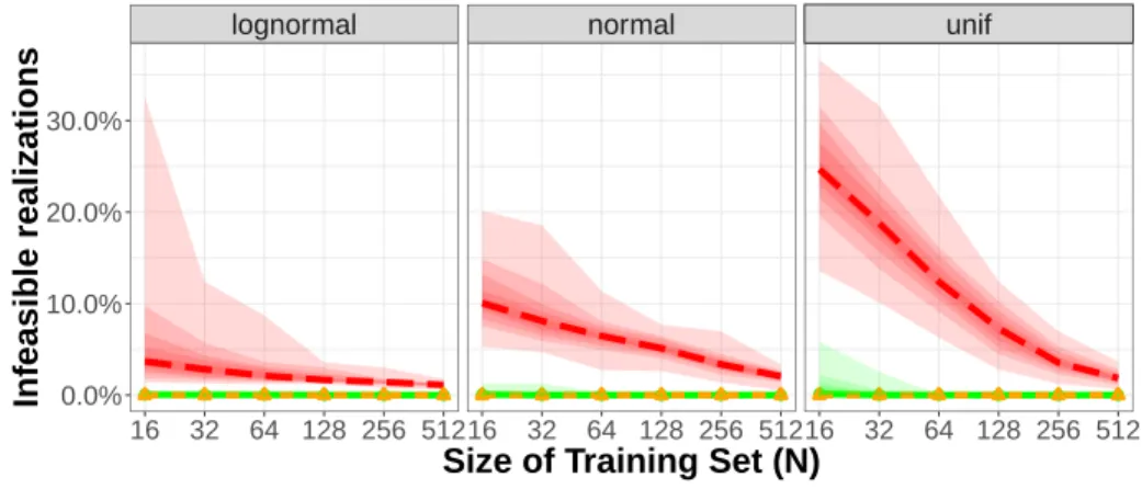
3-4 Capacitated two-stage network inventory management: Average out-of-sample feasibility . . . 108

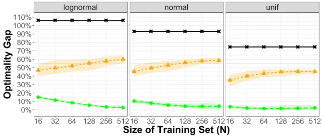
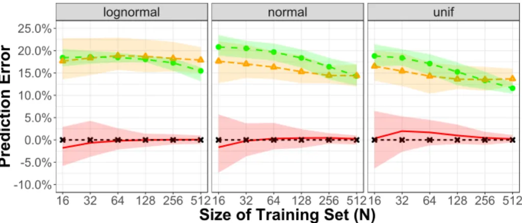
3-5 Capacitated two-stage network inventory management: Optimality gap 109 3-6 Capacitated two-stage network inventory management: Prediction error110 3-7 Medical scheduling: Optimality gap . . . 112

3-8 Medical scheduling: Prediction error . . . 113

4-1 Shipment planning: Average out-of-sample profit. . . 140

4-2 Portfolio management: Average out-of-sample objective . . . 149

(10)

(11)

List of Tables

2.1 Multi-stage stochastic inventory management: Average out-of-sample

cost . . . 65

3.1 Medical scheduling: Computation times. . . 112

4.1 Relationship of four methods. . . 138

4.2 Shipment planning: Statistical significance . . . 141

4.3 Dynamic procurement: Average out-of-sample cost. . . 144

4.4 Dynamic procurement: Statistical significance . . . 145

4.5 Dynamic procurement: Computation times . . . 146

A.1 Multi-stage stochastic inventory management: Average out-of-sample feasibility . . . 195

(12)

(13)

Acknowledgments

First and foremost, I wish to thank Dimitris Bertsimas for advising me these past five years. Thank you for encouraging me to pursue a Ph.D, for your unwavering positivity and support, and for providing the impetus for my growth as a researcher. Beyond teaching me the value of impactful research, you have been a compassionate mentor and friend, and I look forward to continuing our relationship for years to come.

Thank you to my thesis committee members, Vivek Farias and Robert Freund, who played meaningful roles in my doctoral studies. Both of you have given me helpful feedback and advice, both professionally and personally, from which I greatly benefited. I also wish to thank Jim Orlin and Rahul Mazumder for serving on my general exam committee, as well as many other faculty members who have helped me along the way. This thesis is the result of joyful collaborations with Shimrit Shtern and Chris McCord; you are creative, patient, and thoughtful people who have taught me so much, and I am indebted to you both.

Teaching provided me a great deal of entertainment and fun throughout my gradu-ate studies. Thank you to the faculty members who gave me the opportunity to serve as a teaching assistant: Dimitris, Vivek, Shimrit, Georgia Perakis, David Gamarnik, and Dick den Hertog. It was a pleasure to organize the IAP class 15.S60 with Arthur Delarue, Phil Chodrow, and Joey Huchette. Thank you to the ORC staff, Laura Rose and Andrew Carvalho, for everything you did to make all of this possible.

It has been a joy to be a part of the ORC, and I could not have imagined a better intellectual and social community for my graduate studies. I am lucky and grateful to have been supported by old and new friends in Boston: Stuart, Mike, Cristina, Tamar, Jonathan, Haihao, Sam, Ryan, Andy, Ilias, and so many others. In particular, Stuart and Tamar spent countless hours providing feedback on my writing and research, which helped immeasurably. I feel immense love and gratitude for my parents Sandy and Howard, my brother Adam, and countless extended family members who have helped me throughout my life and during graduate school. Thank you all so much.

(14)

This thesis is dedicated to my wife, Rebecca, without whom this would not have been possible. Thank you for going on this journey with me.

(15)

Chapter 1 Introduction

The aim of this introduction is two-fold. First, we provide a background for the reader on multi-stage stochastic linear optimization. To this end, we motivate this important class of decision problems from basic principles (Section 1.1) and provide some select historical results from the literature (Section1.2). Second, we present the main contributions of this thesis in the context of this background and discuss the organization of the subsequent chapters (Section 1.3).

1.1 Problem Setting

This thesis is focused on decision-making under uncertainty in dynamic environments. Specifically, we consider problems faced by organizations in which decisions

x1, . . . , x𝑇

are chosen sequentially over multiple periods of time, as information parameters

(16)

are revealed in each stage. Our goal is to select the decisions in each time period to minimize (or maximize) the total cost (or reward), captured by

𝑐(x1, . . . , x𝑇, 𝜉1, . . . , 𝜉𝑇).

Such decision problems are motivated by practical applications across various branches of operations research, as illustrated by two simple examples:

Example 1. Consider a retailer which aims to manage inventory of a new product over its lifecycle. At the start of each week, the retailer must decide an ordering quantity to replenish its inventory. The demand for the product to the retailer is then revealed over the remaining week, and excess inventory is carried over until the next week. The goal of the retailer is to determine inventory quantities to procure in each week to minimize the total purchasing, holding, and backorder costs.

Example 2. A similar setting is faced by a risk-averse investor who wishes to con-struct and adjust a portfolio of assets to achieve a desirable risk-reward tradeoff over a horizon of many months.

To better understand of this class of decision problems, suppose that we had access to a clairvoyant who could, before any decisions were made, provide the exact values of the information parameters. In this case, the optimal decisions in all of the time periods could ostensibly be found by solving an optimization problem of the form

minimize

x1∈R𝑛1,..., x𝑇∈R𝑛𝑇

𝑐(x1, . . . , x𝑇, 𝜉1, . . . , 𝜉𝑇).

In other words, if the decision-relevant information (such as product demand or stock returns) in each time period were known a priori, then we could determine the optimal decisions across all of the periods ahead of time by solving the above optimization problem.

Of course, in reality, the central challenge is that the decision-relevant information is never known exactly. Thus, the inventory or portfolio decisions in each time period

(17)

must be made in the face of uncertainty. To model this uncertainty, the informa-tion parameters are formalized as random vectors which are associated with a joint probability distribution,

(𝜉₁, . . . , 𝜉_𝑇_{) ∼ P,}

and our revised goal is to choose the decisions which minimize the average cost with respect to the underlying joint probability distribution. To this end, it is perhaps tempting to solve an optimization problem of the form

minimize

x1∈R𝑛1,..., x𝑇∈R𝑛𝑇 EP

[𝑐(x1, . . . , x𝑇, 𝜉1, . . . , 𝜉𝑇)] .

However, as described earlier, we do not want to choose the decisions upfront, but rather choose decisions to adapt to the information learned up to that point. For example, the retailer or investor will reasonably wish to modify their decisions in each period in response to the previous demand or asset returns. More precisely, we actually wish to find decision rules which specify what decision x𝑡(𝜉1, . . . , 𝜉𝑡−1)

to make in each stage as as function of the information observed up to that point. Therefore, the true problem we wish to solve is

minimize

x𝑡:R𝑑1×···×R𝑑𝑡−1→R𝑛𝑡∀𝑡

EP[︀𝑐(x1, x2(𝜉1), . . . , x𝑇(𝜉1, . . . , 𝜉𝑇 −1), 𝜉1, . . . , 𝜉𝑇)]︀ . (OPT)

The central goal of this thesis is develop methods to solve problems of the form (OPT). The decision rules which are produced from the above optimization problem can then be used by managers to make operational decisions. Additionally, the optimal cost of (OPT) can be valuable, for example, in options pricing.

1.2 Background and History

While the cost function can in principle be any arbitrary function of the decisions and information parameters in each time period, we restrict our focus in this thesis

(18)

to cost functions which arise from linear optimization problems. Specifically, our goal in this thesis is to solve (OPT) when the cost function has the form

𝑐 (x1, . . . , x𝑇, 𝜉1, . . . , 𝜉𝑇) = 𝑇 ∑︁ 𝑡=1 (︃ c|_𝑡x𝑡+ min y𝑡∈R𝑟𝑡 {︃ q|_𝑡y𝑡: 𝑡 ∑︁ 𝑠=1 T𝑡,𝑠x𝑠+ 𝑡 ∑︁ 𝑠=1 H𝑡,𝑠𝜉𝑠+ W𝑡y𝑡 ≤ h0𝑡 }︃)︃ ,

where the vectors and matrices which define the cost function are given by c𝑡 ∈ R𝑛𝑡,

q𝑡∈ R𝑟𝑡, T𝑡,𝑠 ∈ R𝑚𝑡×𝑛𝑠, H𝑡,𝑠 ∈ R𝑚𝑡×𝑑𝑠, W𝑡 ∈ R𝑚𝑡×𝑟𝑡, and h0𝑡 ∈ R𝑚𝑡.

Dynamic optimization problems with the above cost functions was first proposed in 1955 by the seminal paper of George Dantzig [35]. We refer to the resulting class of dynamic optimization problems as multi-stage stochastic linear optimization, and [35] is typically credited with precipitating the field of optimization under uncertainty. After 65 years, multi-stage stochastic linear optimization remains one of the leading models for dynamic optimization, widely used by organizations to address fundamen-tal operational planning problems in supply chain management, finance, and energy planning.

Despite the practical importance of this class of dynamic optimization problems, they are notoriously computationally demanding to solve. To see why (OPT) might be challenging from a computational standpoint, let us make two observations. First, we observe that (OPT) requires searching over a general space of decision rules, and is thus is properly characterized as an infinite-dimensional optimization prob-lem. Clearly such a class of optimization problems is computationally demanding in general, as a computer could theoretically require an infinite amount of memory to represent a generic decision rule. Second, we observe that evaluating the expected cost for a given decision rule requires the computation of a multi-dimensional integral. From a complexity standpoint, many problems related to the computing integrals or probabilities over multi-dimensional regions are #𝑃 -hard [43, 41, 22], and solving such problems are considered highly intractable in practice. Indeed, under the cost functions described above, it has been shown that (OPT) with 𝑇 = 1 is #𝑃 -hard [42, 63].

(19)

Motivated by these computational considerations, there is a rich literature of the-ory and algorithms which aim to address (OPT). For example, early work in the 1960s attempted to radically circumvent the computational challenges by replacing the random vectors with their expected values [76, 102, 95]. Subsequent papers in the 1960s and 1970s aimed to characterize the structure of optimal decision rules to (OPT) and its relatives [111,108,44,112,89]. Although there initially was hope that this class of dynamic optimization problems might have optimal decision rules with a simple structure (and thus could potentially be optimized efficiently), this turned out to not be the case. Walkup and Wets [109] showed that piecewise linear decision rules were suboptimal for (OPT) when 𝑇 = 2, and further negative results regarding characterizations of optimal decision rules are underlined by Garastka and Wets [53]. To the best of our knowledge, the structure of optimal decision rules for (OPT) for general distributions remains unknown to this day.

Due to negative results, much research effort has instead focused on approxima-tion schemes for (OPT) using sampling-based and decomposition-based approaches. In a nutshell, such approaches typically employ sampling to construct a tree-based discretization of the true joint probability distribution, and then solve (OPT) us-ing decomposition approaches pioneered by Dantzig and Madansky [36], Birge [25], Rockafellar and Wets [88], Ruszczyński [91], Pereira and Pinto [79], and many oth-ers. For details on sampling-based and decomposition-based approaches, we refer the interested reader to the textbooks [26,98]. A fundamental challenge is that the num-ber of scenarios in a tree-based discretization grows exponentially in the numnum-ber of time periods, which can lead to intractable optimization problems (see, for example, Shapiro and Nemirovski [99, Section 3.2]). An ongoing literature has aimed to mit-igate the explosion of scenarios when discretizing the joint probability distribution [40, 90, 84] or by developing algorithms that are efficient when the random vectors are independently distributed across stages. In a separate direction, there has also been a resurgence of decision-rule based approximations for these stochastic problems [56,74]. Needless to say, the design of methods for obtaining tractable approximations of (OPT) remains an active area of research.

(20)

. . . .

The problem setting and algorithms described above are predicated on the as-sumption that the underlying joint probability distribution is known exactly. In other words, the above discussion assumed that the decision maker who wishes to solve (OPT_{) has perfect knowledge of the underlying joint probability distribution P.}

Of course, a central challenge in applications is that the true distribution is rarely known. Therefore, the traditional practice is to estimate the distribution by fitting historical data to a parametric family of distributions. Any inaccuracies between the estimated distribution and the true distribution will then propagate to suboptimal decision rules. There has been several works which quantify the stability of (OPT) to inaccurate distributions; see, for example, Heitsch et al [66] and Pflug and Pichler [80]. Nonetheless, it is fair to say that the effects of a statistical estimation procedure is generally ignored when assessing the quality of the resulting decisions.

However, the suboptimality resulting from this estimate-then-optimize procedure becomes increasingly significant in this era of big data. Indeed, organizations such as e-commerce retailers, renewable energy providers, and financial institutions increas-ingly have access to rich heterogeneous datasets, which can provide unprecedented insight into how uncertainty unfolds across time. In this context, vital information on the underlying joint probability distribution is foregone when historical sample paths (^𝜉1

1, . . . , ^𝜉1𝑇), . . . , (^𝜉𝑁1 , . . . , ^𝜉𝑁𝑇 ) are aggregated into a simple parametric model

or the correlations across time are ignored. With organizations using to multi-stage stochastic linear optimization to address important challenges faced by society, it is imperative that these organizations effectively harness all of the historical data to make the best possible decisions possible.

1.3 Contributions

This thesis proposes a class of data-driven methods for solving (OPT) when the underlying distribution is unknown. In particular, we develop models and algorithms to transform historical data to address (OPT) which do not require the decision

(21)

maker to impose any parametric modeling assumptions on the underlying probability distribution.

The central theme of this thesis that underpins its contributions is the concept of asymptotic optimality. Specifically, each of the following chapters proposes a new model or algorithm for addressing variants of (OPT) with unknown distributions (Sections 2.3,3.3,4.3), and the main result of each chapter shows the corresponding model or algorithm is guaranteed to provide a near-optimal approximations of (OPT) when the sample size 𝑁 tends to infinity (Sections2.4,3.4,4.4). In doing so, our aim is to empower organizations to effectively harness the rapidly-increasing availability of historical data to make near-optimal dynamic decisions under uncertainty.

The contributions of this thesis came to fruition by viewing (OPT) through the perspective of robust optimization. Specifically, our approaches for solving (OPT) are based on solving a robust optimization problem with multiple uncertainty sets. By drawing connections between these traditionally separate fields, we are able to leverage theoretical and algorithmic advances from robust optimization to analyze and approximate the proposed approach. To the best of our knowledge, there was no similar work in the literature which used robust optimization as a tool for solving multi-stage stochastic linear optimization. We showcase the potential of our con-tributions through simulated experiments in the context of inventory management, shipment planning, hospital scheduling, and finance.

In greater detail, this thesis makes the following contributions.

A Data-Driven Approach to Multi-Stage Stochastic Linear Optimization

In Chapter2, we propose a new data-driven approach, based on robust optimization, for solving (OPT) with unknown probability distributions. Specifically, we propose approximating (OPT) by solving an optimization problem of the form

minimize 1 𝑁 𝑁 ∑︁ 𝑗=1 max (𝜁1,...,𝜁𝑇)∈𝒰 𝑗 𝑁 𝑐(x1, x2(𝜁1), . . . , x𝑇(𝜁1, . . . , 𝜁𝑇 −1), 𝜁1, . . . , 𝜁𝑇), (SRO)

(22)

where 𝒰_𝑁𝑗 is an uncertainty set that is constructed around the historical sample path (^𝜉𝑗₁, . . . , ^𝜉𝑗_𝑇). Hence, this approach uses robust optimization as a tool for solving multi-stage stochastic linear optimization directly from data. More specifically, we obtain decision rules and estimate the optimal cost of Problem (OPT) by solving (SRO). The main result of the chapter (Theorem 1) shows, under mild assumptions and ap-propriate construction of the uncertainty sets, that the above model is asymptotically optimal ; that is, the optimal cost of (SRO) converges to that of (OPT) as 𝑁 → ∞. To the best of our knowledge, this is the first data-driven approach to (OPT) which is asymptotically optimal when uncertainty is arbitrarily correlated across time.

While (SRO) is computationally demanding to solve exactly, we show it can be tractably approximated to reasonable accuracy by extending techniques from the field of robust optimization (such as linear decision rules and finite adaptability). We demonstrate their practical value through numerical experiments on stylized data-driven inventory management problems.

Two-Stage Sample Robust Optimization

In Chapter3, we develop a simple approximation algorithm for (SRO) for the partic-ular case of 𝑇 = 1.1 _{The algorithm consists of optimizing overlapping linear decision}

rules, one for the uncertainty set around each data point. We show that the proposed algorithm can be tractably solved as a linear optimization problem with size that scales linearly in the number of data points.

The main result of this chapter (Theorem 6) shows that the approximation al-gorithm itself is asymptotically optimal, meaning that the optimal cost and optimal decisions from the approximation algorithm are guaranteed to converge to those of (OPT) as the number of data points tends to infinity. To the best of our knowledge, this is the first solution approach for such a class of data-driven robust optimiza-tion problems which simultaneously offers the key attractive properties (scalability and asymptotic optimality) which have underpinned the success of the sample

aver-1_{Under the cost function described in Section}_1.2_{, (}_OPT_{) with 𝑇 = 1 is known in the literature} as a two-stage problem. We follow this convention to be consistent with the literature.

(23)

age approximation in two-stage problems. We demonstrate the practical value of our method through examples from network inventory management and hospital schedul-ing.

Dynamic Optimization with Side Information

In Chapter 4, we develop an extension of (SRO) to address dynamic optimization problems with side information, of the form

minimize

x𝑡:R𝑑1×···×R𝑑𝑡−1→R𝑛𝑡∀𝑡

EP[︀𝑐(x1, x2(𝜉1), . . . , x𝑇(𝜉1, . . . , 𝜉𝑇 −1), 𝜉1, . . . , 𝜉𝑇) | 𝛾 = ¯𝛾]︀ .

This class of stochastic problems naturally arises in many applications in which or-ganizations have additional side information (such as the brand or color of a new product, or recent asset returns and prices of relevant options) which can be used to predict future uncertainty (product demand, or asset returns). We address these problems by using predictive machine learning methods (such as 𝑘-nearest neighbors, kernel regression, and random forests) to weight the costs in (SRO).

The main result of this chapter (Theorem 11) shows that the machine learning-based extension of (SRO) is asymptotically optimal for the above stochastic problems with side information. The key innovation behind our proof is a new measure concen-tration result, which shows for the first time that an empirical conditional probability distribution that is constructed using certain machine learning methods will, as more data is obtained, converge to the true conditional probability distribution with respect to the type-1 Wasserstein distance.

Finally, we describe an extension the general-purpose approximation scheme from Chapter3to the multi-stage setting, which is computationally tractable and produces high-quality solutions for dynamic problems with many stages. Across a variety of examples in shipment planning, inventory management, and finance, our method achieves improvements of up to 15% over alternatives and requires less than one minute of computation time on problems with twelve stages.

(24)

(25)

Chapter 2 A Data-Driven Approach to

Multi-Stage Stochastic Linear

Optimization

In this chapter, we propose a new data-driven approach for addressing multi-stage stochastic linear optimization problems with unknown distributions. The approach consists of solving a robust optimization problem that is constructed from sample paths of the underlying stochastic process. As more sample paths are obtained, we prove that the optimal cost of the robust problem converges to that of the underlying stochastic problem. To the best of our knowledge, this is the first data-driven ap-proach for multi-stage stochastic linear optimization which is asymptotically optimal when uncertainty is arbitrarily correlated across time. Finally, we develop approxima-tion algorithms for the proposed approach by extending techniques from the robust optimization literature, and demonstrate their practical value through numerical ex-periments on stylized data-driven inventory management problems.

2.1 Introduction

In the traditional formulation of linear optimization, one makes a decision which minimizes a known objective function and satisfies a known set of constraints. Linear

(26)

optimization has, by all measures, succeeded as a framework for modeling and solving numerous real world problems. However, in many practical applications, the objective function and constraints are unknown at the time of decision making. To incorporate uncertainty into the linear optimization framework, George Dantzig [35] proposed partitioning the decision variables across multiple stages, which are made sequentially as more uncertain parameters are revealed. This formulation is known today as multi-stage stochastic linear optimization, which has become an integral modeling paradigm in many applications (e.g., supply chain management, energy planning, finance) and remains a focus of the stochastic optimization community [26, 98].

In practice, decision makers increasingly have access to historical data which can provide valuable insight into future uncertainty. For example, consider a manufac-turer which sells short lifecycle products. The manufacmanufac-turer does not know a joint probability distribution of the demand over a new product’s lifecycle, but has access to historical demand trajectories over the lifecycle of similar products. Another ex-ample is energy planning, where operators must coordinate and commit to production levels throughout a day, the output of wind turbines is subject to uncertain weather conditions, and data on historical daily wind patterns is increasingly available. Other examples include portfolio management, where historical asset returns over time are available to investors, and transportation planning, where data comes in the form of historical ride usage of transit and ride sharing systems over the course of a day. Such historical data provides significant potential for operators to better understand how uncertainty unfolds through time, which can in turn be used for better planning.

When the underlying probability distribution is unknown, data-driven approaches to multi-stage stochastic linear optimization traditionally follow a two-step procedure. The historical data is first fit to a parametric model (e.g., an autoregressive moving average process), and decisions are then obtained by solving a multi-stage stochastic linear optimization problem using the estimated distribution. The estimation step is considered essential, as techniques for solving multi-stage stochastic linear optimiza-tion (e.g., scenario tree discretizaoptimiza-tion) generally require knowledge of the correlaoptimiza-tion structure of uncertainty across time; see [98, Section 5.8]. A fundamental difficulty

(27)

in this approach is choosing a parametric model which will accurately estimate the underlying correlation structure and lead to good decisions.

Nonparametric data-driven approaches to multi-stage stochastic linear optimiza-tion where uncertainty is correlated across time are surprisingly scarce. [81] propose a nonparametric estimate-then-optimize approach based on applying a kernel den-sity estimator to the historical data, which enjoys asymptotic optimality guarantees under a variety of strong technical conditions. [60] present another nonparametric ap-proach wherein the conditional distributions in stochastic dynamic programming are estimated using kernel regression. [73] discuss nonparametric path-grouping heuris-tics for constructing scenario trees from historical data. In the case of multi-stage stochastic linear optimization, to the best of our knowledge, there are no previous non-parametric data-driven approaches which are asymptotically optimal in the presence of time-dependent correlations. Moreover, in the absence of additional assumptions on the estimated distribution or on the problem setting, multi-stage stochastic linear optimization problems are notorious for being computationally demanding.

The main contribution of this chapter is a new data-driven approach for multi-stage stochastic linear optimization that is asymptotically optimal, even when uncer-tainty is arbitrarily correlated across time. In other words, we propose a data-driven approach for addressing multi-stage stochastic linear optimization with unknown dis-tributions that (i ) does not require any parametric modeling assumptions on the correlation structure of the underlying probability distribution, and (ii ) converges to the underlying multi-stage stochastic linear optimization problem as the size of the dataset tends to infinity. Such an asymptotic optimality guarantee is of practical importance, as it ensures that the approach offers a near-optimal approximation of the underlying stochastic problem in the presence of big data.

Our approach for multi-stage stochastic linear optimization is based on robust optimization. Specifically, given sample paths of the underlying stochastic process, the proposed approach consists of constructing and solving a multi-stage robust linear optimization problem with multiple uncertainty sets. The main result of this chapter (Theorem 1) establishes, under certain assumptions, that the optimal cost of this

(28)

robust optimization problem converges nearly to that of the stochastic problem as the number of sample paths tends to infinity. While this robust optimization prob-lem is computationally demanding to solve exactly, we provide evidence that it can be tractably approximated to reasonable accuracy by leveraging approximation tech-niques from the robust optimization literature. To the best of our knowledge, there was no similar work in the literature which addresses multi-stage stochastic linear optimization by solving a sequence of robust optimization problems.

The chapter is organized as follows. Section 2.2 introduces multi-stage stochastic linear optimization in a data-driven setting. Section2.3presents the new data-driven approach to multi-stage stochastic linear optimization. Section 2.4 states the main asymptotic optimality guarantees. Section 2.5 presents two examples of approxi-mation algorithms by leveraging techniques from robust optimization. Section 2.6

discusses implications of our asymptotic optimality guarantees in the context of Wasserstein-based distributionally robust optimization. Section2.7demonstrates the out-of-sample performance and computational tractability of the proposed method-ologies in computational experiments. Section 2.8 offers concluding thoughts. All technical proofs are relegated to the attached appendices.

2.1.1 Related literature

Originating with [100] and [9], robust optimization has been widely studied as a gen-eral framework for decision-making under uncertainty, in which “optimal" decisions are those which perform best under the worst-case parameter realization from an “uncertainty set". Beginning with the seminal work of [8], robust optimization has been viewed with particular success as a computationally tractable framework for addressing multi-stage problems. Indeed, by restricting the space of decision rules, a stream of literature showed that multi-stage robust linear optimization problems can be solved in polynomial time by using duality-based reformulations or cutting-plane methods. For a modern overview of decision-rule approximations, we refer the reader to [37, 54, 7, 10]. A variety of non-decision rule approaches to solving multi-stage robust optimization have been proposed as well, such as [116, 117, 114, 55].

(29)

Despite its computational tractability for multi-stage problems, a central critique of traditional robust optimization is that it does not aspire to find solutions which perform well on average. Several works have aimed to quantify the quality of solu-tions from multi-stage robust linear optimization from the perspective of multi-stage stochastic linear optimization [30, 13, 15]. By and large, it is fair to say that stage robust linear optimization is viewed today as a distinct framework from multi-stage stochastic linear optimization, aiming to find solutions with good worst-case as opposed to good average performance.

Providing a potential tradeoff between the stochastic and robust frameworks, dis-tributionally robust optimization has recently received significant attention. First proposed by [92], distributionally robust optimization models the uncertain param-eters with a probability distribution, but the distribution is presumed to be un-known and contained in an ambiguity set of distributions. Even though single-stage stochastic optimization is generally intractable, the introduction of ambiguity can surprisingly emit tractable reformulations [38, 113]. Consequently, the extension of distributionally robust optimization to multi-stage decision making is an active area of research, including [21] for multi-stage distributionally robust linear optimization with moment-based ambiguity sets.

There has been a proliferation of data-driven constructions of ambiguity sets which offer various probabilistic performance guarantees, including those based on the 𝑝-Wasserstein distance for 𝑝 ∈ [1, ∞) [82,77], phi-divergences [6,4,104], and statistical hypothesis tests [16]. Many of these data-driven approaches have since been applied to the particular case of two-stage distributionally robust linear optimization, including [69] for phi-divergence and [61] for 𝑝-Wasserstein ambiguity sets when 𝑝 ∈ [1, ∞). To the best of our knowledge, no previous work has demonstrated whether such distributionally robust approaches, if extended to solve multi-stage stochastic linear optimization (with three or more stages) directly from data, retain their asymptotic optimality guarantees.

In contrast to the above literature, our motivation for robust optimization in this chapter is not to find solutions which perform well on the worst-case realization

(30)

in an uncertainty set, are risk-averse, or have finite-sample probabilistic guarantees. Rather, our proposed approach to multi-stage stochastic linear optimization adds robustness to the historical data as a tool to avoid overfitting as the number of data points tends to infinity. In this spirit, our work is perhaps closest related to several papers in the context of machine learning [115,96], which showed that adding robustness to historical data can be used to develop machine learning methods which have nonparametric performance guarantees when the solution space (of classification or regression models) is not finite-dimensional. To the best of our knowledge, this work is the first to apply this use of robust optimization in the context of multi-stage stochastic linear optimization to achieve asymptotic optimality without restricting the space of decision rules.

As far as we are aware, our data-driven approach of averaging over multiple un-certainty sets is novel in the context of multi-stage stochastic linear optimization, and its asymptotic optimality guarantees do not follow from existing literature. [115] con-sidered averaging over multiple uncertainty sets to establish convergence guarantees for predictive machine learning methods, drawing connections with distributionally robust optimization and kernel density estimation. Their convergence results require that the objective function is continuous, the underlying distribution is continuous, and there are no constraints on the support. Absent strong assumptions on the problem setting and on the space of decision rules (which in general can be discontin-uous), these properties do not hold in multi-stage problems. [46] provide feasibility guarantees on robust constraints over unions of uncertainty sets with the goal of approximating ambiguous chance constraints using the Prohorov metric. Their prob-abilistic guarantees require that the constraint functions have a finite VC-dimension [46, Theorem 5], an assumption which does not hold in general for two- or multi-stage problems [47]. In this work, we instead establish general asymptotic optimality guarantees for the proposed data-driven approach for multi-stage stochastic linear op-timization by developing new bounds for distributionally robust opop-timization with the 1-Wasserstein ambiguity set and connections with nonparametric support estimation [39].

(31)

Under a particular construction of the uncertainty sets, we show that the pro-posed data-driven approach to multi-stage stochastic linear optimization can also be interpreted as distributionally robust optimization using the ∞-Wasserstein ambi-guity set (see Section 2.6). However, the asymptotic optimality guarantees in this work do not make use of this interpretation, as there were surprisingly few previ-ous convergence results for this ambiguity set, even in single-stage settings. Indeed, when an underlying distribution is unbounded, the ∞-Wasserstein distance between an empirical distribution and true distribution is always infinite [58] and thus does not converge to zero as more data is obtained. Therefore, it is not possible to develop measure concentration guarantees for the ∞-Wasserstein distance (akin to those of [50]) which hold in general for light-tailed but unbounded probability distributions. Consequently, the proof techniques used by [77, Theorem 3.6] to establish conver-gence guarantees for the 1-Wasserstein ambiguity set do not appear to extend to the ∞-Wasserstein ambiguity set. As a byproduct of the results in this chapter, we ob-tain asymptotic optimality guarantees for distributionally robust optimization with the ∞-Wasserstein ambiguity set under the same mild probabilistic assumptions as [77] for the first time.

2.1.2 Notation

We denote the real numbers by R, the nonnegative real numbers by R+, and the

integers by Z. Lowercase and uppercase bold letters refer to vectors and matrices. We assume throughout that ‖·‖ refers to an ℓ𝑝-norm in R𝑑, such as ‖v‖1 =∑︀𝑑_𝑖=1|𝑣𝑖|

or ‖v‖∞ = max𝑖∈[𝑑]|𝑣𝑖|. We let ∅ denote the empty set, int(·) be the interior of a

set, and [𝐾] be shorthand for the set of consecutive integers {1, . . . , 𝐾}. Throughout the chapter, we let 𝜉 := (𝜉₁, . . . , 𝜉_𝑇_{) ∈ R}𝑑 _{denote a stochastic process with a joint}

probability distribution P, and assume that ^𝜉1, . . . , ^𝜉𝑁 are independent and identically distributed (i.i.d.) samples from that distribution. Let P𝑁 _{:= P × · · · × P denote the}

𝑁 -fold probability distribution over the historical data. We let 𝑆 ⊆ R𝑑 denote the support of P, that is, the smallest closed set where P(𝜉 ∈ 𝑆) = 1. The extended real numbers are defined as ¯_{R := R∪{−∞, ∞}, and we adopt the convention that ∞−∞ =}

(32)

∞. The expectation of a measurable function 𝑓 : R𝑑 _{→ R applied to the stochastic}

process is denoted by E[𝑓 (𝜉)] = EP[𝑓 (𝜉)] = EP[max{𝑓 (𝜉), 0}] − EP[max{−𝑓 (𝜉), 0}].

Finally, for any set 𝒵 ⊆ R𝑑, we let 𝒫(𝒵) denote the set of all probability distributions on R𝑑 _{which satisfy Q(𝜉 ∈ 𝒵) ≡ E}

Q[I{𝜉 ∈ 𝒵}] = 1.

2.2 Problem Setting

We consider multi-stage stochastic linear optimization problems with 𝑇 ≥ 1 stages. The uncertain parameters observed over the time horizon are represented by a stochas-tic process 𝜉 := (𝜉₁, . . . , 𝜉_𝑇_{) ∈ R}𝑑 _{with an underlying joint probability distribution,}

where 𝜉_𝑡 _{∈ R}𝑑𝑡 _{is a random variable that is observed immediately after the decision}

in stage 𝑡 is selected. We assume throughout that the random variables 𝜉₁, . . . , 𝜉_𝑇 may be correlated. A decision rule x := (x1, . . . , x𝑇) is a collection of policies which

specify what decision to make in each stage based on the information observed up to that point. More precisely, a policy in each stage is a measurable function of the form x𝑡: R𝑑1× · · · × R𝑑𝑡−1 → R𝑛𝑡−𝑝𝑡 × Z𝑝𝑡. We use the shorthand notation x ∈ 𝒳 to

denote such decision rules.

In multi-stage stochastic linear optimization, our goal is to find a decision rule which minimizes a linear cost function in expectation while satisfying a system of linear inequalities almost surely. These problems are represented by

minimize x∈𝒳 E [︃ _𝑇 ∑︁ 𝑡=1 c𝑡(𝜉) · x𝑡(𝜉1, . . . , 𝜉𝑡−1) ]︃ subject to 𝑇 ∑︁ 𝑡=1 A𝑡(𝜉)x𝑡(𝜉1, . . . , 𝜉𝑡−1) ≤ b(𝜉) a.s. (2.1)

Following standard convention, we assume that the problem parameters c1(𝜉) ∈

R𝑛1, . . . , c𝑇(𝜉) ∈ R𝑛𝑇, A1(𝜉) ∈ R𝑚×𝑛1, . . . , A𝑇(𝜉) ∈ R𝑚×𝑛𝑇, and b(𝜉) ∈ R𝑚 are

affine functions of the stochastic process.

In this chapter, we assume that the underlying joint probability distribution of the stochastic process is unknown. Instead, our information comes from historical

(33)

data of the form

^

𝜉𝑗 ≡ (^𝜉𝑗₁, . . . , ^𝜉𝑗_𝑇), 𝑗 = 1, . . . , 𝑁.

We refer to each of these trajectories as a sample path of the stochastic process. This setting corresponds to many real-life applications. For example, consider managing the inventory of a new short lifecycle product, in which production decisions must be made over the product’s lifecycle. In this case, each sample path represents the historical sales data observed over the lifecycle of a comparable product. Further examples are readily found in energy planning and finance, among many others. We assume that ^𝜉1_{, . . . , ^}_𝜉𝑁 _{are independent and identically distributed (i.i.d.) realizations}

of the stochastic process 𝜉 ≡ (𝜉₁, . . . , 𝜉_𝑇). Our goal in this chapter is a general-purpose, nonparametric sample-path approach for solving Problem (2.1) in practical computation times.

We will also assume that the support of the stochastic process is unknown. For example, in inventory management, an upper bound on the demand, if one exists, is generally unknown. On the other hand, we often have partial knowledge on the underlying support. For example, when the stochastic process captures the demand for a new product or the energy produced by a wind turbine, it is often the case that the uncertainty will be nonnegative. To allow any partial knowledge on the support to be incorporated, we assume knowledge of a convex superset Ξ ⊆ R𝑑of the support of the underlying joint distribution, that is, P(𝜉 ∈ Ξ) = 1.

2.3 Sample Robust Optimization

We now present the proposed data-driven approach, based on robust optimization, for solving multi-stage stochastic linear optimization. First, we construct an uncertainty set 𝒰_𝑁𝑗 ⊆ Ξ around each sample path, consisting of realizations 𝜁 ≡ (𝜁₁, . . . , 𝜁_𝑇) which are slight perturbations of ^𝜉𝑗 ≡ (^𝜉𝑗₁, . . . , ^𝜉𝑗_𝑇). Then, we optimize for decision rules by averaging over the worst-case costs from each uncertainty set, and require that the decision rule is feasible for all realizations in all of the uncertainty sets. Formally, the

(34)

proposed approach is the following: minimize x∈𝒳 1 𝑁 𝑁 ∑︁ 𝑗=1 sup 𝜁∈𝒰_𝑁𝑗 𝑇 ∑︁ 𝑡=1 c𝑡(𝜁) · x𝑡(𝜁1, . . . , 𝜁𝑡−1) subject to 𝑇 ∑︁ 𝑡=1 A𝑡(𝜁)x𝑡(𝜁1, . . . , 𝜁𝑡−1) ≤ b(𝜁) ∀𝜁 ∈ ∪𝑁𝑗=1𝒰 𝑗 𝑁. (2.2)

In contrast to traditional robust optimization, Problem (2.2) involves averaging over multiple uncertainty sets. Thus, the explicit goal here is to obtain decision rules which perform well on average while simultaneously not overfitting the historical data. We note that Problem (2.2) only requires that the decision rules are feasible for the realizations in the uncertainty sets. These feasibility requirements are justified when the overlapping uncertainty sets encompass the variability of future realizations of the uncertainty; see Section 2.4.

Out of the various possible constructions of the uncertainty sets, our investigation shall henceforth be focused on uncertainty sets constructed as balls of the form

𝒰𝑗_𝑁 := {︁𝜁 ≡ (𝜁₁, . . . , 𝜁_𝑇) ∈ Ξ : ‖𝜁 − ^𝜉𝑗‖ ≤ 𝜖𝑁

}︁ ,

where 𝜖𝑁 ≥ 0 is a parameter which controls the size of the uncertainty sets. The

parameter is indexed by 𝑁 to allow for the size of the uncertainty sets to change as more data is obtained. The rationale for this particular uncertainty set is three-fold. First, it is conceptually simple, requiring only a single parameter to both estimate the expectation in the objective and the support of the distribution in the constraints. Second, under appropriate choice of the robustness parameter, we will show that Problem (2.2) with these uncertainty sets provides a near-optimal approximation of Problem (2.1) in the presence of big data (see Section 2.4). Finally, the uncertainty sets are of similar structure, which can be exploited to obtain tractable reformulations (see Section 2.5).

Our approach, in a nutshell, uses robust optimization as a tool for solving multi-stage stochastic linear optimization directly from data. More specifically, we obtain

(35)

decision rules and estimate the optimal cost of Problem (2.1) by solving Problem (2.2). We refer the proposed data-driven approach for solving multi-stage stochastic linear optimization problems as sample or sample-path robust optimization. As mentioned previously, the purpose of robustness is to ensure that resulting decision rules do not overfit the historical sample paths. To illustrate this role performed by robustness, we consider the following example.

Example 3. Consider a supplier which aims to satisfy uncertain demand over two phases at minimal cost. The supplier selects an initial production quantity at $1 per unit after observing preorders, and produces additional units at $2 per unit after the regular orders are received. To determine the optimal production levels, we wish to solve

minimize _{E [𝑥}2(𝜉1) + 2𝑥3(𝜉1, 𝜉2)]

subject to 𝑥2(𝜉1) + 𝑥3(𝜉1, 𝜉2) ≥ 𝜉1+ 𝜉2 a.s.

𝑥2(𝜉1), 𝑥3(𝜉1, 𝜉2) ≥ 0 a.s.

(2.3)

The output of the optimization problem are decision rules, 𝑥2 : R → R and 𝑥3 :

R2 → R, which specify what production levels to choose as a function of the de-mands observed up to that point. The joint probability distribution of the demand process (𝜉1, 𝜉2) ∈ R2 is unknown, and the supplier’s knowledge comes from historical

demand realizations of past products, denoted by ( ^𝜉1

1, ^𝜉21), . . . , ( ^𝜉1𝑁, ^𝜉2𝑁). For the sake

of illustration, suppose we attempted to approximate Problem (2.3) by choosing the decision rules which perform best when averaging over the historical data without any robustness. Such a sample average approach amounts to solving

minimize 1 𝑁 𝑁 ∑︁ 𝑗=1 (︁ 𝑥2( ^𝜉𝑗1) + 2𝑥3( ^𝜉𝑗1, ^𝜉 𝑗 2) )︁ subject to 𝑥2( ^𝜉𝑗1) + 𝑥3( ^𝜉𝑗1, ^𝜉 𝑗 2) ≥ ^𝜉 𝑗 1+ ^𝜉 𝑗 2 ∀𝑗 ∈ [𝑁 ] 𝑥2( ^𝜉𝑗1), 𝑥3( ^𝜉𝑗1, ^𝜉 𝑗 2) ≥ 0 ∀𝑗 ∈ [𝑁 ].

Suppose that the random variable 𝜉1 for preorders has a continuous distribution. In

(36)

optimal decision rule for the above optimization problem is 𝑥2(𝜉1) = ⎧ ⎪ ⎨ ⎪ ⎩ ^ 𝜉𝑗₁+ ^𝜉𝑗₂, if 𝜉1 = ^𝜉 𝑗 1 for 𝑗 ∈ [𝑁 ], 0, otherwise; 𝑥3(𝜉1, 𝜉2) = 0.

Unfortunately, these decision rules are nonsensical with respect to Problem (2.3). Indeed, the decision rules will not result in feasible decisions for the true stochastic problem with probability one. Moreover, the optimal cost of the above optimization problem will converge almost surely to E[𝜉1 + 𝜉2] as the number of sample paths

𝑁 tends to infinity, which can in general be far from that of the stochastic prob-lem. Clearly, such a sample average approach results in overfitting, even in big data settings, and thus provides an unsuitable approximation of Problem (2.3).

The key takeaway from this chapter is that this overfitting phenomenon in the above example is eliminated by adding robustness to the historical data. In partic-ular, we will show in the following section that when the robustness parameter 𝜖𝑁

is chosen appropriately, Problem (2.2) converges to a near-optimal approximation of Problem (2.1) as more data is obtained, without requiring any parametric assump-tions on the stochastic process nor restricassump-tions on the space of decision rules.

2.4 Asymptotic Optimality

In this section, we present theoretical guarantees showing that Problem (2.2) pro-vides a near-optimal approximation of Problem (2.1) in the presence of big data. In Section 2.4.1, we describe the assumptions used in the subsequent convergence results. In Section 2.4.2, we present the main result of this chapter (Theorem 1), which establishes asymptotic optimality of the proposed data-driven approach. In Section2.4.3, we interpret Theorem 1through several examples. In Section 2.4.4, we present asymptotic feasibility guarantees.

(37)

2.4.1 Assumptions

We begin by introducing our assumptions which will be used for establishing asymp-totic optimality guarantees. First, we will assume that the joint probability distribu-tion of the stochastic process satisfies the following light-tail assumpdistribu-tion:

Assumption 1. There exists a constant 𝑎 > 1 such that 𝑏 := E [exp(‖𝜉‖𝑎)] < ∞.

For example, this assumption is satisfied if the stochastic process has a multivariate Gaussian distribution, and is not satisfied if the stochastic process has a multivariate exponential distribution. Importantly, Assumption1does not require any parametric assumptions on the correlation structure of the random variables across stages, and we do not assume that the coefficient 𝑎 > 1 is known.

Second, we will assume that the robustness parameter 𝜖𝑁 is chosen to be strictly

positive and decreases to zero as more data is obtained at the following rate:

Assumption 2. There exists a constant 𝜅 > 0 such that 𝜖𝑁 := 𝜅𝑁

− 1

max{3,𝑑+1}_.

In a nutshell, Assumption 2provides a theoretical requirement on how to choose the robustness parameter to ensure that Problem (2.2) will not overfit the historical data (see Example 3 from Section 2.3). The rate also provides practical guidance on how the robustness parameter can be updated as more data is obtained. We note that, for many of the following results, the robustness parameter can decrease to zero at a faster rate; nonetheless, we shall impose Assumption 2 for all our results for simplicity.

Finally, our convergence guarantees for Problem (2.2) do not require any restric-tions on the space of decision rules. Our analysis will only require the following assumption on the problem structure:

Assumption 3. There exists a 𝐿 ≥ 0 such that, for all 𝑁 ∈ N, the optimal cost of Problem (2.2) would not change if we added the following constraints:

sup 𝜁∈∪𝑁 𝑗=1𝒰 𝑗 𝑁 ⃦ ⃦x𝑡(𝜁1, . . . , 𝜁𝑡−1) ⃦ ⃦≤ sup 𝜁∈∪𝑁 𝑗=1𝒰 𝑗 𝑁 𝐿(1 + ‖𝜁‖) ∀𝑡 ∈ [𝑇 ].

(38)

This assumption says that there always exists a near-optimal decision rule to Problem (2.2) where the decisions which result from realizations in uncertainty sets are bounded by the largest realization in the uncertainty sets. Moreover, this is a mild assumption that we find can be easily verified in many practical examples. In Appendix A.1, we show that every example presented in this chapter satisfies this assumption.

2.4.2 Main result

We now present the main result of this chapter (Theorem 1), which shows that the optimal cost of Problem (2.2) nearly converges to the optimal cost of Problem (2.1) as 𝑁 → ∞. For notational convenience, let 𝐽* be the optimal cost of Problem (2.1),

̂︀

𝐽𝑁 be the optimal cost of Problem (2.2), and 𝑆 ⊆ Ξ be the support of the underlying

joint probability distribution of the stochastic process.

Our main result presents tight asymptotic lower and upper bounds on the optimal cost ̂︀𝐽𝑁 of Problem (2.2). First, let 𝐽

¯ be defined as the maximal optimal cost of any chance-constrained variant of the multi-stage stochastic linear optimization problem:

𝐽 ¯ := lim𝜌↓0 minimizex∈𝒳 , ˜𝑆⊆Ξ E [︃ _𝑇 ∑︁ 𝑡=1 c𝑡(𝜉) · x𝑡(𝜉1, . . . , 𝜉𝑡−1)I {︁ 𝜉 ∈ ˜𝑆}︁ ]︃ subject to 𝑇 ∑︁ 𝑡=1 A𝑡(𝜁)x𝑡(𝜁1, . . . , 𝜁𝑡−1) ≤ b(𝜁) ∀𝜁 ∈ ˜𝑆 P (︁ 𝜉 ∈ ˜𝑆)︁≥ 1 − 𝜌.

We observe that the above limit must exist, as the optimal cost of the chance-constrained optimization problem is monotone in 𝜌. We also observe that 𝐽

¯ is always a lower bound on 𝐽*_{, since for every 𝜌 > 0, adding the constraint P(𝜉 ∈ ˜}𝑆) = 1 to the above chance-constrained optimization problem would increase its optimal cost to 𝐽*.1

1_{The definition does not preclude the possibility that 𝐽}

¯ is equal to −∞ or ∞. However, we do not expect either of those values to occur outside of pathological cases; see Section2.4.3. The same remark applies to the upper bound ¯𝐽 .

(39)

Second, let ¯𝐽 be the optimal cost of the multi-stage stochastic linear optimiza-tion problem with an addioptimiza-tional restricoptimiza-tion that the decision rules are feasible on an expanded support: ¯ 𝐽 := lim 𝜌↓0 minimizex∈𝒳 ¯ E [︃ _𝑇 ∑︁ 𝑡=1 c𝑡(𝜉) · x𝑡(𝜉1, . . . , 𝜉𝑡−1) ]︃ subject to 𝑇 ∑︁ 𝑡=1 A𝑡(𝜁)x𝑡(𝜁1, . . . , 𝜁𝑡−1) ≤ b(𝜁) ∀𝜁 ∈ Ξ : dist(𝜁, 𝑆) ≤ 𝜌.

We remark that the limit as 𝜌 tends down to zero must exist as well, since the optimal cost of the above optimization problem with expanded support is monotone in 𝜌. Note also that the expectation in the objective function has been replaced with ¯_{E[·], which} we define here as the local upper semicontinuous envelope of an expectation, i.e.,

¯

E[𝑓 (𝜉)] := lim𝜖→0E[sup𝜁∈Ξ:‖𝜁−𝜉‖≤𝜖𝑓 (𝜉)]. We similarly observe that ¯𝐽 is an upper

bound on 𝐽*, since the above optimization problem involves additional constraints and an upper envelope of the objective function.

Our main result is the following:

Theorem 1. Suppose Assumptions 1, 2, and 3 _{hold. Then, P}∞-almost surely we have

𝐽

¯ ≤ lim inf𝑁 →∞ 𝐽̂︀𝑁 ≤ lim sup_{𝑁 →∞} 𝐽̂︀𝑁 ≤ ¯𝐽 .

Proof. See Appendix C.2.

The above theorem provides assurance that the proposed data-driven approach becomes a near-optimal approximation of multi-stage stochastic linear optimization in the presence of big data. Note that Theorem1 holds in very general cases; for ex-ample, it does not require boundedness on the decisions or random variables, requires no parametric assumptions on the correlations across stages, and holds when the decisions contain both continuous and integer components. Moreover, these asymp-totic bounds for Problem (2.2) do not necessitate imposing any restrictions on the space of decision rules. To the best of our knowledge, such nonparametric asymptotic

(40)

optimality guarantees for a sample-path approach to multi-stage stochastic linear optimization are the first of their kind when uncertainty is correlated across time.

Our proof of Theorem1is based on a new uniform convergence result (Theorem2) which establishes a general relationship for arbitrary functions between the in-sample worst-case cost and the expected out-of-sample cost over the uncertainty sets. We state this theorem below due to its independent interest.

Theorem 2. If Assumptions 1 and 2 hold, then there exists a ¯_{𝑁 ∈ N, P}∞-almost surely, such that

E[︀𝑓 (𝜉)I {︀𝜉 ∈ ∪𝑁𝑗=1𝒰 𝑗 𝑁}︀]︀ ≤ 1 𝑁 𝑁 ∑︁ 𝑗=1 sup 𝜁∈𝒰_𝑁𝑗 𝑓 (𝜁) + 𝑀𝑁 sup 𝜁∈∪𝑁 𝑗=1𝒰 𝑗 𝑁 |𝑓 (𝜁)|

for all 𝑁 ≥ ¯_{𝑁 and all measurable functions 𝑓 : R}𝑑_{→ R, where 𝑀}

𝑁 := 𝑁

− 1

(𝑑+1)(𝑑+2)_{log 𝑁 .}

Proof. See Appendix A.3.

We note that our proofs of Theorems 1 and 2 also utilize a feasibility guarantee (Theorem 3) which can be found Section2.4.4.

2.4.3 Examples where ¯

𝐽 − 𝐽

¯

is zero or strictly positive

In general, we do not expect the gap between the lower and upper bound in Theo-rem 1to be large. In fact, we will now show that the lower and upper bounds can be equal, i.e., 𝐽

¯ = ¯𝐽 , in which case the optimal cost of Problem (2.2) provably converges to the optimal cost of Problem (2.1). We provide such an example by revisiting the stochastic inventory management problem from Example 3. The following proposi-tion, in combination with Theorem 1, shows that adding robustness to the historical data provably overcomes the overfitting phenomenon discussed in Section2.3. Proposition 1. For Problem (2.3), 𝐽

¯ = 𝐽

*_{. If there is an optimal 𝑥}*

2 : R → R for

Problem (2.3) which is continuous, then ¯𝐽 = 𝐽*.

The proof of this proposition, found in Appendix A.4, holds for any underlying probability distribution which satisfies Assumption 1.

(41)

While the above example shows that the lower and upper bounds may be equal, unless further restrictions are placed on the space of multi-stage stochastic linear optimization problems, they can have a nonzero gap. In the following, we present three examples that provide intuition on the situations in which this gap may be strictly positive. Our first example presents a problem in which the lower bound 𝐽

¯ is equal to 𝐽* but is strictly less than the upper bound ¯𝐽 .

Example 4. Consider the single-stage stochastic problem

minimize

𝑥1∈Z

𝑥1

subject to 𝑥1 ≥ 𝜉1 a.s.,

where the random variable 𝜉1 is governed by the probability distribution P(𝜉1 > 𝛼) =

(1 − 𝛼)𝑘 for fixed 𝑘 > 0, and Ξ = [0, 2]. We observe that the support of the random variable is 𝑆 = [0, 1], and thus the optimal cost of the stochastic problem is 𝐽* = 1. We similarly observe that the lower bound is 𝐽

¯ = 1 and the upper bound, due to the integrality of the first stage decision, is ¯𝐽 = 2. If 𝜖𝑁 = 𝑁−

1

3, then we prove in

AppendixA.5 that the bounds in Theorem 1 are tight under different choices of 𝑘:

Range of 𝑘 Result

𝑘 ∈ (0, 3) _P∞ (︂

𝐽

¯ < lim inf𝑁 →∞ 𝐽̂︀𝑁 = lim sup_{𝑁 →∞} 𝐽̂︀𝑁 = ¯𝐽

)︂ = 1

𝑘 = 3 _P∞

(︂ 𝐽

¯ = lim inf𝑁 →∞ 𝐽̂︀𝑁 < lim sup_{𝑁 →∞} 𝐽̂︀𝑁 = ¯𝐽

)︂ = 1

𝑘 ∈ (3, ∞) _P∞ (︂

𝐽

¯ = lim inf𝑁 →∞ 𝐽̂︀𝑁 = lim sup_{𝑁 →∞} 𝐽̂︀𝑁 < ¯𝐽

)︂ = 1

This example shows that gaps can arise between the lower and upper bounds when mild changes in the support of the underlying probability distribution lead to signifi-cant changes in the optimal cost of Problem (2.1). Moreover, this example illustrates that each of the inequalities in Theorem 1can hold with equality or strict inequality when the feasibility of decisions depends on random variables that have not yet been realized.

(42)

Our second example presents a problem in which the upper bound ¯𝐽 is equal to 𝐽* but is strictly greater than the lower bound 𝐽

¯. This example deals with the special case in which any chance constrained version of a stochastic problem leads to a decision which is infeasible for the true stochastic problem.

Example 5. Consider the single-stage stochastic problem

minimize

x1∈R2

𝑥12

subject to 𝜉1(1 − 𝑥12) ≤ 𝑥11 a.s.

0 ≤ 𝑥12≤ 1,

where 𝜉1 ∼ Gaussian(0, 1) and Ξ = R. The constraints are satisfied only if 𝑥12 = 1,

and so the optimal cost of the stochastic problem is 𝐽* = 1. Since there is no expectation in the objective and Ξ equals the true support, we also observe that

¯

𝐽 = 1. However, we readily observe that there is always a feasible solution to the sample robust optimization problem (Problem (2.2)) where 𝑥12 = 0, and therefore

𝐽

¯ = ̂︀𝐽𝑁 = 0 for all 𝑁 ∈ N.

Our third and final example demonstrates the necessity of the upper semicontin-uous envelope ¯_{E[·] in the definition of the upper bound.}

Example 6. Consider the two-stage stochastic problem

minimize

𝑥2:R→Z E [𝑥

2(𝜉1)]

subject to 𝑥2(𝜉1) ≥ 𝜉1 a.s.,

where 𝜃 ∼ Bernoulli(0.5) and 𝜓 ∼ Uniform(0, 1) are independent random variables, 𝜉1 = 𝜃𝜓, and Ξ = [0, 1]. An optimal decision rule 𝑥*2 : R → Z to the stochastic

problem is given by 𝑥*₂(𝜉1) = 0 for all 𝜉1 ≤ 0 and 𝑥*2(𝜉1) = 1 for all 𝜉1 > 0, which

implies that 𝐽* = 1₂. It follows from similar reasoning that 𝐽 ¯ =

1

2. Since Ξ equals the

support of the random variable, the only difference between the stochastic problem and the upper bound is that the latter optimizes over the local upper semicontinuous envelope, and we observe that lim𝑁 →∞𝐽̂︀𝑁 = ¯𝐽 = ¯E[𝑥*2(𝜉1)] = 1.

(43)

In each of the above examples, we observe that the bounds in Theorem1are tight, in the sense that the optimal cost of Problem (2.2) converges either to the lower bound or the upper bound. This provides some indication that the bounds in Theorem 1

offer an accurate depiction of how Problem (2.2) can behave in the asymptotic regime. On the other hand, the above examples which illustrate a nonzero gap seem to require intricate construction, and future work may identify (sub-classes) of Problem (2.1) where the equality of the bounds can be ensured.

2.4.4 Feasibility guarantees

We conclude Section2.4by discussing out-of-sample feasibility guarantees for decision rules obtained from Problem (2.2). Recall that Problem (2.2) finds decision rules which are feasible for each realization in the uncertainty sets. However, one cannot guarantee that these decision rules will be feasible for realizations outside of the uncertainty sets. Thus, a pertinent question is whether a decision rule obtained from approximately solving Problem (2.2) is feasible with high probability. To address the question of feasibility, we leverage classic results from detection theory.

Let 𝑆𝑁 := ∪𝑁𝑗=1𝒰 𝑗

𝑁 be shorthand for the union of the uncertainty sets. We say

that a decision rule is 𝑆𝑁-feasible if

𝑇

∑︁

𝑡=1

A𝑡(𝜁)x𝑡(𝜁1, . . . , 𝜁𝑡−1) ≤ b(𝜁) ∀𝜁 ∈ 𝑆𝑁.

In other words, the set of feasible decision rules to Problem (2.2) are exactly those which are 𝑆𝑁-feasible. Our subsequent analysis utilizes the following (seemingly

tau-tological) observation: for any decision rule that is 𝑆𝑁-feasible,

P (︃ _𝑇 ∑︁ 𝑡=1 A𝑡(𝜉)x𝑡(𝜉1, . . . , 𝜉𝑡−1) ≤ b(𝜉) )︃ ≥ P (𝜉 ∈ 𝑆𝑁) ,

where P(𝜉 ∈ 𝑆𝑁) is shorthand for P(𝜉 ∈ 𝑆𝑁 | ^𝜉1, . . . , ^𝜉𝑁). Indeed, this inequality

follows from the fact that a decision rule which is 𝑆𝑁-feasible is definitionally feasible

(44)

probability that 𝜉 ∈ 𝑆𝑁.

We have thus transformed the analysis of feasible decision rules for Problem (2.2) to the problem of analyzing the performance of 𝑆𝑁 as an estimate for the support 𝑆 of

a stochastic process. Interestingly, this nonparametric estimator for the support of a joint probability distribution has been widely studied in the statistics literature, with perhaps the earliest results coming from [39] in detection theory. Since then, the per-formance of 𝑆𝑁 as a nonparametric estimate of 𝑆 has been studied with applications

in cluster analysis and image recognition [72,93]. Leveraging this connection between stochastic optimization and support estimation, we obtain the following guarantee on feasibility.

Theorem 3. Suppose Assumptions 1 and 2 _{hold. Then, P}∞-almost surely we have

lim 𝑁 →∞ (︃ 𝑁𝑑+11 (log 𝑁 )𝑑+1 )︃ P(𝜉 ̸∈ 𝑆𝑁) = 0.

Proof. See Appendix A.6.

Intuitively speaking, Theorem 3 provides a guarantee that any feasible decision rule to Problem (2.2) will be feasible with high probability on future data when the number of sample paths is large. To illustrate why robustness is indeed necessary to achieve such feasibility guarantees, we recall from Example3 that decision rules may prohibitively overfit the data and be infeasible with probability one if the robustness parameter 𝜖𝑁 is set to zero.

2.5 Approximation Techniques

In the previous section, we developed theoretical guarantees which demonstrated that Problem (2.2) provides a good approximation of multi-stage stochastic linear opti-mization when the number of sample paths is large. In this section, we demonstrate that Problem (2.2) can be addressed using approximation techniques from the field of robust optimization. Specifically, we show that two decision-rule approximation

Dynamic optimization in the age of big data

Dynamic

Optimization in the Age of Big Data

by

Bradley

Eli Sturt

B.S.,

University of Illinois at Urbana-Champaign (2014)

Submitted

to the Sloan School of Management

in

partial fulfillment of the requirements for the degree of

Doctor

of Philosophy in Operations Research

at

the

MASSACHUSETTS

INSTITUTE OF TECHNOLOGY

May 2020

○

c

Massachusetts Institute of Technology 2020. All rights reserved.

Author . . . .

Sloan School of Management

April 23, 2020

Certified by . . . .

Dimitris Bertsimas

Boeing Professor of Operations Research

Thesis Supervisor

Accepted by . . . .

Patrick Jaillet

Dugald C. Jackson Professor, Department of Electrical Engineering and

Computer Science

Co-director, Operations Research Center

Dynamic Optimization in the Age of Big Data

by

Bradley Eli Sturt

Abstract

Contents

List of Figures

List of Tables

Acknowledgments

Chapter 1

Introduction

1.1

Problem Setting

1.2

Background and History

1.3

Contributions

Chapter 2

A Data-Driven Approach to

Multi-Stage Stochastic Linear

Optimization

2.1

Introduction

2.1.1

Related literature

2.1.2

Notation

2.2

Problem Setting

2.3

Sample Robust Optimization

2.4

Asymptotic Optimality

2.4.1

Assumptions

2.4.2

Main result

2.4.3

Examples where ¯

𝐽 − 𝐽

¯

is zero or strictly positive

2.4.4

Feasibility guarantees

2.5

Approximation Techniques