HAL Id: hal-02525906
https://hal.archives-ouvertes.fr/hal-02525906v3
Preprint submitted on 11 Feb 2021HAL is a multi-disciplinary open access archive for the deposit and dissemination of sci-entific research documents, whether they are pub-lished or not. The documents may come from teaching and research institutions in France or abroad, or from public or private research centers.
L’archive ouverte pluridisciplinaire HAL, est destinée au dépôt et à la diffusion de documents scientifiques de niveau recherche, publiés ou non, émanant des établissements d’enseignement et de recherche français ou étrangers, des laboratoires publics ou privés.
Relaxing door-to-door matching reduces passenger
waiting times: a workflow for the analysis of driver GPS
traces in a stochastic carpooling service
Panayotis Papoutsis, Safa Fennia, Constant Bridon, Tarn Duong
To cite this version:
Panayotis Papoutsis, Safa Fennia, Constant Bridon, Tarn Duong. Relaxing door-to-door matching reduces passenger waiting times: a workflow for the analysis of driver GPS traces in a stochastic carpooling service. 2021. �hal-02525906v3�
Relaxing door-to-door matching reduces passenger waiting
times: a workflow for the analysis of driver GPS traces in a
stochastic carpooling service
Panayotis Papoutsis∗1,2,3, Safa Fennia3, Constant Bridon3, and Tarn Duong3 1Department of Computing and Mathematics, Nantes Central Engineering School,
F-44300, France
2Jean Leray Mathematics Laboratory, University of Nantes, F-44300, France 3Department of Data Science-GIS, Ecov, F-44200, France
Abstract
Carpooling has the potential to transform itself into a mass transportation mode by aban-doning its adherence to deterministic passenger-driver matching for door-to-door journeys, and by adopting instead stochastic matching on a network of fixed meeting points. Stochastic matching is where a passenger sends out a carpooling request at a meeting point, and then waits for the arrival of a self-selected driver who is already travelling to the requested meeting point. Crucially there is no centrally dispatched driver. Moreover, the carpooling is assured only between the meeting points, so the onus is on the passengers to travel to/from them by their own means. Thus the success of a stochastic carpooling service relies on the con-vergence, with minimal perturbation to their existing travel patterns, to the meeting points which are highly frequented by both passengers and drivers. Due to the innovative nature of stochastic carpooling, existing off-the-shelf workflows are largely insufficient for this purpose. To fill the gap in the market, we introduce a novel workflow, comprising of a combination of data science and GIS (Geographic Information Systems), to analyse driver GPS traces. We implement it for an operational stochastic carpooling service in south-eastern France, and we demonstrate that relaxing door-to-door matching reduces passenger waiting times. Our workflow provides additional key operational indicators, namely the driver flow maps, the driver flow temporal profiles and the driver participation rates.
Keywords: data science, stochastic matching, GIS, meeting point, network
1
Introduction
Carpooling has seen an explosion of utilisation in recent years [Furuhata et al., 2013]. There are many underlying reasons for this, with concerns ranging from greenhouse gas emissions and air pollution to road congestion to land use, as well as economic costs [Shaheen et al., 2016]. It also attracts intense interest since carpooling is a crucial element of almost all development plans for smart cities [Ghoseiri,2012]. A broad definition of carpooling involves a driver sharing their journey with passengers. In this paper we employ a narrower definition. We additionally
require that a non-professional driver would have undertaken their journey for their own reasons, regardless of whether the passengers would have been present or not. The driver may receive payment to offset the costs of the use of their vehicle, but the profit motive is non-existent or at least not their primary motivation [Zhu,2020]. Hence we do not consider taxi-like services (such as Uber, Lyft and Kapten etc.) to be carpooling services as they employ professional drivers who create a journey in response to a passenger request and are then paid the market rate for the service rendered.
Due to the altruistic nature of carpooling, service providers tend to be small, local, non-profit organisations. Though it does not preclude viable business models arising from carpooling with non-professional drivers: the market leader BlaBlaCar levies a commission fee for facilitating the matching of drivers and passengers [Shaheen et al., 2017]. This matching is managed by a centralised platform, which we call deterministic matching since a known driver is assigned in advance to collect the passenger. This deterministic matching is highly successful for infrequent, long distance, pre-reserved carpooling journeys, as witnessed by BlaBlaCar’s status as a unicorn start-up company (a market capitalisation of at least 1000 million USD). Despite the success of deterministic passenger-driver matching in this market, attempts to export it other carpooling markets have not resulted in the same level of market penetration. This is most notable for frequent, short distance journeys (from 10 to 40 km roughly), which comprise the bulk of daily home-work commutes, and so carpooling remains a marginal practice in this market.
This paper focuses on short-distance, non-reserved carpooling, and it is what we refer to when employing ‘carpooling’ without any qualifiers. The advent of mass carpooling depends crucially on incentivising drivers and passengers to converge onto highly frequented meeting points (hotspots) along their door-to-door journeys [Stiglic et al.,2015]. This type of incentivi-sation is well-established for a bus network where passengers embark/disembark only at the fixed bus stops. Thus mass carpooling requires a paradigm shift from considering carpooling as an exclusively private means of transport to a closer alignment to public transport models [Cooper, 2007].
Continuing with the public transport model, the meeting points are not defined informally between passengers and drivers, but are decided in consultation with local government authorities so that they respond to the mobility requirements in the local area, taking into account various factors such as aggregated traffic flow, socioeconomic characteristics, pedestrian accessibility, local government regulations, etc. For our purposes, we consider that the identification of the meeting hotspots has been carried out beforehand. These meeting points are then connected to each other to define carpooling lines, which have massification potential, like traditional bus lines [Stiglic et al.,2015,Li et al.,2018].
Like a bus service, no pre-reservations are required, as a passenger makes an ad hoc carpooling request at a meeting point, and this request for the desired destination is communicated to all passing drivers in real-time via an electronic sign on the side of a highly frequented main road. Unlike for deterministic passenger-driver matching mentioned above, a specific driver is not assigned to the passenger by a centralised platform, but the decision to collect a passenger at the meeting point is made spontaneously by a self-selected driver. Since the actual driver who collects the passenger is not known deterministically in advance, but is only known to be drawn from the population of drivers, this is known as stochastic matching. Due to the inherent variability of these driver arrivals, stochastic matching is only feasible when employed in conjunction with a network of highly frequented meeting points.
sparsely covered by the recent comprehensive review of general carpooling and taxi-like services over the past two decades [Wang and Yang,2019]. So there are few off-the-shelf workflows which are suitable for the analysis of the data arising from a stochastic carpooling service. We introduce a data science-GIS workflow which fills this gap in the market. Its main data source is the GPS traces, and its secondary sources are the meeting point locations, the origin-destination matrices, the route finder API and the base maps. Data wrangling/geoprocessing are then applied to these data sources, with the critical geoprocessing step being the topological simplification of the GPS traces onto the carpooling network. This topological simplification is essential to be able to mutualise GPS traces which share common arrival times at the meeting points. From these simplified GPS traces, we can produce the waiting times. The latter allow us to assert that stochastic matching at meeting points leads to reduced passenger waiting times in comparison to door-to-door matching. In addition to the waiting times, other outputs from this workflow are the driver flow maps, the driver flow profiles, and the driver participation rates. These additional outputs are obtained at low marginal cost but which are important elements for evidence-based decision making in a stochastic carpooling service.
In Section 2 we present the theoretical reasons why door-to-door matching is insufficient to ensure a regular carpooling service. In Section 3 we detail our data science-GIS workflow for the analysis of GPS traces. In Section 4, we apply this workflow to an operational stochastic carpooling service to produce the passenger waiting times and the other outputs. We end with some concluding remarks.
2
Door-to-door matching is an obstacle to mass carpooling
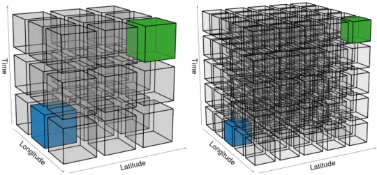
As alluded to in the introduction, door-to-door matching of complete trajectories from the origin to the destination is a structural obstacle to the transformation of carpooling to a mass transit service. To illustrate the difficulties of passenger-driver matching in space and in time for door-to-door trajectories, we can represent it with partition of a 3D cube divided into smaller sub-cubes, where the x-axis is the longitude, the y-axis the latitude and the z-axis the time, as shown in Figure 1. On the left, there are 9 sub-cubes, where each sub-cube represents the origin/destination of a door-to-door trajectory. The blue sub-cube in the lower left represents all the trajectories whose origins are, say, within a 5 km radius around a residential neighbourhood between 07:00 and 09:00 on Tuesday, and the green sub-cube the trajectories whose destination are within a 5 km radius of the workplace between 08:00 and 10:00 on Tuesday. So for two trajectories to match spatio-temporally in a door-to-door sense, they must share the same sub-cube for the origin, and similarly for the destination: this condition is met by the 1 pair of green and blue sub-cubes among all possible 27 pairs of sub-cubes. On the right, the conditions for a door-to-door matching are stricter, say the origin is 1 km within the residential neighbourhood during 07:00 to 07:30, and the destination is 1 km within the workplace during 08:30 to 09:00. This represents 1 pair out of 125 pairs of sub-cubes. Thus stricter door-to-door matching leads to fewer drivers being available to share their trajectories with passengers.
To supplement the heuristic observations for door-to-door matching in Figure 1, we demon-strate that the probability that two users (i.e. a driver and a passenger) share the same origin and destination at the same time decreases rapidly as the spatio-temporal matching conditions become more stringent. For the sake of simplicity, we suppose that the origin and destination for a driver and a passenger are both represented by independent random variables which are uni-form over all sub-cubes in Figure1. Let UOd and UDd be the origin and destination of a driver, and
Figure 1: Spatio-temporal door-to-door matching fragments the population of mutualisable tra-jectories. (Left) Relaxed matching conditions. (Right) Restricted matching conditions. Blue sub-cube represents the origin (residential neighbourhood), green the destination (workplace), and trajectories which share the same origin and destination sub-cubes are considered to be door-to-door matches.
likewise UOp, UDp for a passenger. These quantities are all uniform random variables U ({1, . . . , n}) where n is the number of sub-cubes in Figure 1. Then the probability of a door-to-door match between the driver and passenger is p(n) = P(UOp = UOd, U
p
D = UDd). Since an exact formula for
this probability is difficult to obtain, we approximate it by a Monte Carlo re-sampling method. That is, we generate 1000 samples of UOp, UOd, UDp, UDd and the probability of a door-to-door match is approximated as ˆ p(n) = 1 1000 1000 X i=1 1 1
1{UO,ip = UO,id , UD,ip = UD,id }
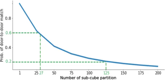
where 111{·} is the indicator function. Figure 2 is the graph of the number of sub-cubes n versus the approximate probability of a door-to-door match ˆp(n). If there is only 1 sub-cube (i.e. no spatio-temporal constraints) the probability of a match is 1. This probabilistic certainty decreases rapidly as the spatio-temporal constraints are added: for 27 sub-cubes, this probability is 0.6, and for 125 sub-cubes, it falls to 0.2.
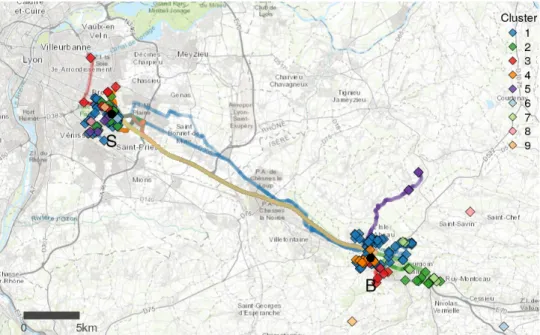
The previous analysis was based on the synthetic uniformly distributed origins and destina-tions. For a more realistic example, we analyse some data generated by an operational carpooling service. Our example is the ‘Lane’ carpooling service (lanemove.com) operated by Ecov, in con-junction with Instant System (instant-system.com), since May 2018 in the peri-urban regions around Lyon in south-eastern France. Our main data source is the GPS traces of drivers, which can be considered to be a form of crowd-sourced data collection [Lee and Liang, 2011]. Pas-senger GPS traces are more difficult to obtain, and as we are not able to replicate exactly the synthetic example of passenger-driver matching above, so we use door-to-door matching of driver GPS traces to illustrate the diminishing probabilities. Since these GPS traces provide highly de-tailed spatio-temporal information, we are able to determine the number of strict door-to-door matches which also pass by two meeting points, as well as the number of matches when door-to-door matching is relaxed. For an illustrative example in Figure 3, we analyse 121 GPS traces
Figure 2: Probability of door-to-door matches for uniformly distributed drivers and passengers, as a function of the number of sub-cube partition classes. Higher number of sub-cubes represent more stringent spatio-temporal matching conditions.
of drivers who travelled from the Bourgoin meeting point (solid black circle labelled B) to the St-Priest meeting point (solid black circle labelled S) in the Lane carpooling service during the morning operating hours (06:30 to 09:00) for the work week 2019-11-25 to 2019-12-01. A hierar-chical clustering with complete linkage was carried out on the spatial locations of these origins and destinations. The dissimilarity matrix used for this hierarchical clustering is composed of the Euclidean distance between the 4-vector comprising the (origin longitude, origin latitude, destination longitude, destination latitude) of each trajectory. This dissimilarity takes into ac-count both the origin and the destination, but not the intermediate GPS points as these actual route taken is not critical for our purposes. We cut the dendrogram at h = 6000 to yield 9 spatial clusters. These clusters are represented with the different colours. So GPS traces with the same colour can be considered as door-to-door matches with each other.
The number of GPS traces per cluster is given in Table 1: as cluster 1 contains 75% of the mutualisable traces, this leaves the other 25% spread sparsely over the other 8 clusters, fragmenting the supply of the carpooling trajectories to passengers.
Door-to-door cluster 1 2 3 4 5 6 7 8 9 Total
Number of GPS traces 76 15 7 9 4 1 7 1 1 121
Table 1: Spatio-temporal door-to-door matching fragments the number of mutualisable trajecto-ries in the Bourgoin > St-Ptrajecto-riest carpooling line, during its morning operating hours 06:30–09:00, from 2018-11-25 to 2018-12-01. The first line is the door-to-door cluster label and the second line is the number of traces in each cluster.
To quantify the augmentation of the carpooling potential by relaxing door-to-door matching, we compare the door-to-door cluster with the largest cardinality (76 traces) from Table 1 to the number of the trajectories (121 traces) which coincide with this carpooling line regardless of their true origin and destination. These counts are an empirical equivalent of Figure 1: the left corresponds to the 121 meeting point (i.e. relaxed door-to-door) matches, whereas the right the
Figure 3: Spatio-temporal door-to-door matching fragments the number of mutualisable trajec-tories in an operational stochastic carpooling service. The clusters of GPS traces of door-to-door matches are colour coded, with the GPS points as the solid circles, and the origins/destinations as the solid diamonds. The meeting points are the solid black circles, denoted B = Bourgoin, S = St-Priest.
76 door-to-door matches. Thus meeting point matching represents an increase of 45 traces or 59% of the carpooling driver potential due to relaxing door-to-door matching.
Furthermore,Stiglic et al. [2015] andLi et al.[2018] provide more complex synthetic models to affirm that meeting points are essential to the feasibility of the mass carpooling services, and assert that it is almost impossible for a carpooling service to be based on door-to-door spatio-temporal matching.
Whilst these examples demonstrate that incentivising drivers to converge to meeting points, rather than relying on door-to-door matching, increases the potential pool of mutualisable jour-neys, we have not yet demonstrated that this leads to reduced waiting times. This would be straightforward for the synthetic examples but this is not the case for empirically observed drivers and passengers journeys. In the next section we introduce a general workflow which indeed allows us to confirm these reduced waiting times for empirical GPS traces.
3
Data science-GIS workflow for the analysis of GPS traces
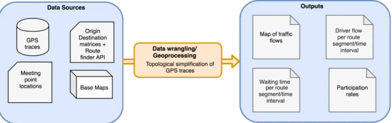
The GPS traces analysis workflow is illustrated in Figure4. The left rectangle of Figure4contains the main data sources: the GPS traces, the meeting point locations, the origin-destination matrices, the route finder API and the base maps. The first two are supplied in-house by the carpooling service provider, the origin-destination matrices are usually supplied by a third party which has carried out a mobility survey (e.g. a national statistical agency INSEE [2018]), the route finder API is provided by a GPS navigation operator (e.g. TomTom [2019]), and the base maps are accessed from a cartography provider (e.g. OpenStreetMap contributors [2019]). There are specialised data wrangling techniques specific to spatial databases, known collectively
as geoprocessing, and these are carried out, in conjunction with traditional data wrangling, in the central rectangle. The critical geoprocessing task concerns the topological simplification of the GPS traces onto the carpooling network. Whilst GPS traces are a rich source of information of driver behaviour, they are voluminous and complex. Our approach is based on network analysis tools [Guidotti et al., 2017] and complexity reduction/harmonisation algorithms [Douglas and Peucker, 2011]. This topological simplification is essential to be able to mutualise GPS traces which share common arrival times at the carpooling meeting points. Once these GPS traces are in a suitable format, we are able to produce the required outputs in the right rectangle, namely the predicted waiting times, the driver flow maps, the driver flow temporal profiles and the driver participation rates.
Figure 4: Data science-GIS workflow for the analysis of driver GPS traces in stochastic carpooling service. (Left) Spatio-temporal input data sources. (Centre) Data wrangling and geoprocessing tasks. (Right) Generated outputs.
3.1 Data sources
Our primary data source are the driver GPS traces. A GPS trace is represented by an `-sequence of triplets X = {(Xi, Yi, Ti)}`i=1where (Xi, Yi) are the longitude, latitude coordinates of the GPS
sensor at the ith timestamp Ti. We have n GPS traces X1, . . . , Xn in the data collection period.
The m meeting point locations are represented by their GPS coordinates M1, . . . , Mm. The
origin-destination matrix is such that its (j, k)th entry is the number of journeys from jth origin to the kthdestination. In addition to the origin-destination matrix, we have the GPS coordinates of the origins and the destinations. Whilst it is common that they coincide, this is not required for our workflow. The base maps are graphics files of maps of the study area, which facilitate the fast and accurate map rendering at any desired scale.
3.2 Data wrangling/geoprocessing
From the m meeting points M1, . . . , Mm, a directed graph is constructed where the meeting
points are the nodes, and an edge is drawn between the two nodes if carpooling between these two meeting points is guaranteed by the service provider. Thus a carpooling line is represented by an acyclic sub-graph with at least two nodes.
The crucial data wrangling/geoprocessing process applied to the GPS traces is the topological simplification of GPS traces on a carpooling line. Around each of the m meeting points, a buffer zone of 1 km radius is drawn to obtain B(M1), . . . , B(Mm). The intersection of the buffer zones
and the GPS trace, X ∩ B(M1), . . . , X ∩ B(Mm), is m sub-sequences of the GPS points of X.
For those meeting points with non-empty intersections, we consider that the driver is able to collect a passenger at these points without onerous detours.
This spatial intersection only considers the spatial proximity of the driver to a passenger at a meeting point. For the carpooling to succeed, they also need to be in temporal proximity. Among the spatial intersections X ∩B(M1), . . . , X ∩B(Mm), we examine the corresponding timestamps
and retain only those in a suitably restrained time interval. If this reduced set of spatio-temporal intersections is non-empty then we proceed to the last data wrangling/geoprocessing step.
We compute the closest GPS points in X to the meeting points Mj, as defined by XMj = {(Xk, Yk, Tk) : k = argmin1≤i≤`k((Xi, Yi) − Mjk}, j = 1, . . . , m. From this closest point XMj, we can extract the corresponding timestamp to be an estimate of the arrival time at the meeting point Mj. As an example, if the meeting points M1, M2 form the carpooling line {M1 > M2},
and if the GPS trace X has well-defined estimated arrival times at M1 and M2, then we are
able to reduce the complexity of the GPS trace. That is the ` points of X can be reduced to the sequence of 4 points
˜
X(M1, M2) = {(X1, Y1, T1) > XM1 > XM2 > (X`, Y`, T`)}
where (X1, Y1, T1) is the driver origin and (X`, Y`, T`) is the driver destination. With this
simpli-fied trace ˜X(M1, M2), we are still able to determine if the driver can fulfil a passenger request at
a given time on the carpooling line {M1 > M2}. The complex topology of X is thus simplified
by retaining a small number of key derived indicators [Lee and Liang,2011].
We repeat these data wrangling/geoprocessing steps for all n GPS traces. The result is a reduced set of ˜n GPS traces which correspond to the driver journeys which closely resemble the spatio-temporal characteristics of the likely passenger requests along the carpooling line.
3.3 Outputs
For the first output in the workflow in Figure4, if we visualise the GPS traces of the reduced set of ˜
n meeting point matches with the base maps, then we obtain a map of the driver flow that matches to the passengers in the carpooling line, as in Figure 3. For the second output in the workflow, suppose that the initial time interval of interest is divided into nT sub-intervals τj, j = 1, . . . , nT
since we wish to quantify the driver flow at a higher temporal resolution. Computing the driver flows f (τj), j = 1, . . . , nT, is straightforward as it only requires an enumeration of the simplified
GPS traces whose estimated arrival times fall within each sub-interval τj. That is, the driver flow for the carpooling line {M1 > M2} during the time interval τj is
f (τj, M1, M2) = #{i : ˜Xi(M1, M2) ∈ τj, i = 1, . . . , ˜n}. (1)
For the third output in the workflow, let W (t) be the waiting time until the driver arrival for a carpool request made at time t. For stochastic carpooling, since a specific driver is not dispatched to the given passenger, the problem is equivalent to the arrival time of the first driver from the population of available drivers. Assuming a Poissonian driver arrival process, the waiting time and the driver flow are inversely proportional to each other, W (t) ∝ len(τj)/f(τj)
where t ∈ τj and len(τj) is the length of the time interval τj. For simplicity, we set the constant of
proportionality to 1 as this corresponds to the assumption that all geolocated drivers are willing to respond to a carpooling request. It is a reasonable assumption that the vast majority of geolocated drivers are willing to pick up a passenger, according to unpublished evidence supplied
by Ecov. Thus for the carpooling line {M1 > M2}, the passenger waiting times for the time
interval τj, j = 1, . . . , nT, are
W (τj, M1, M2) = len(τj)/f (τj, M1, M2). (2)
For the fourth output in the workflow, the driver participation rate is P = n1/n0where n1 is
the total number of the drivers who are motivated to carpool in response to a passenger request, and n0 is the total numbers of drivers who undertake journeys in the same geographical region as the carpooling service. Both n1 and n0 are difficult to define and to estimate precisely. We
propose that ˜n, calculated above as the number of drivers who share their geolocation, to be our proxy for n1, as the vast majority of carpooling journeys are assured by drivers who are willing to share their geolocation.
To enumerate all n0 drivers in the same geographical region as the carpooling network is
difficult since the GPS traces for all drivers are not available. Our proxy (˜n0) is derived from
inferring likely trajectories from the reference destination matrix. Usually this origin-destination matrix is provided at the county-level, but this is insufficiently detailed to decide if the drivers match with the meeting points on the carpooling lines. So we infer likely trajectories. These inferred likely trajectories are determined as the fastest route from the origins (county centroids) to the destinations (county centroids) by a route finder API. We employ a route finder API rather than an explicit model-based methodology, e.g. Tang et al.[2016], to infer these most likely routes. Model-based methods are the product of extensive theoretical and empirical work, and these tend to be difficult to access due to their proprietary nature. They also tend to be limited to dense urban regions, which are not the target regions for stochastic carpooling. Thus ˜
n0 is the sum of the driver flow from all origin-destination pairs whose likely trajectories coincide
with the carpooling lines. The driver participation rate for a carpooling line {M1> M2} is
˜
P = ˜n/˜n0 (3)
where ˜n =PnT
j=1f (τj, M1, M2) from Equation (1).
Since there is no comparable door-to-door carpooling service operating concurrently with the meeting-point stochastic carpooling service, a direct comparison of empirical passenger waiting times is not possible. Instead, we propose an indirect comparison in three stages: (i) extract all driver GPS traces which connect two meeting points in a restrained time interval, as the meeting point matches, (ii) extract the largest hierarchical cluster of these GPS traces to serve as the door-to-door matches, and (iii) compute the driver flows using Equation (1) for both sets of matches, and then convert them using Equation (2) to passenger waiting time predictions.
In addition to the waiting times as an output, there are also the driver flow maps, the driver flow temporal profiles, and the driver participation rates. All these outputs are useful in understanding the transport mix of the local area as well as the market penetration of the carpooling into the transport mix.
4
Case study of an operational stochastic carpooling service
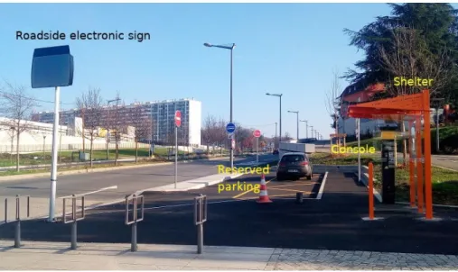
Our case study focuses on the Lane carpooling service introduced earlier. Before we progress further into the data analysis of the driver GPS traces, we describe the operational details of this stochastic carpooling service. The physical meeting points require an integrated infrastructure to facilitate this real-time stochastic matching, as illustrated in Figure 5. The orange structure
on the right functions like a bus shelter to provide protection from inclement weather whilst the passenger waits, and a prominent visual point of reference for drivers on the road. The passenger makes a carpooling request on the console (the green device with a horizontal yellow stripe). This request is displayed on the electronic sign on the roadside. In this configuration, the electronic sign is located close to the meeting point, but this can vary considerably according to the local geographical characteristics. A driver who wishes to embark the passenger in response to their request is able to do so safely in the reserved parking place.
Figure 5: Configuration of a physical meeting point for the ‘Lane’ carpooling service. The orange structure is like a bus shelter. A passenger notifies potential drivers of their carpooling request using the console, which is then displayed on the roadside electronic sign. A driver can safely embark the passenger in the reserved parking place. Reproduced with permission from Ecov.
4.1 Topological simplification of GPS traces on a carpooling line
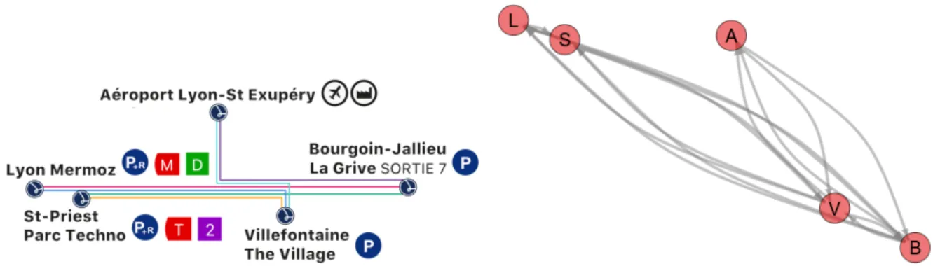
The schematic diagram of the carpooling lines in the Lane network is shown on the left of Figure6. The visual similarities of the schematic of this carpooling service with those associated with bus or train services is deliberately designed to induce the perception of carpooling as a form of public transport. There are 5 physical meeting points (Lyon Mermoz, St-Priest Parc Techno, Aéroport Lyon-St Exupéry, Villefontaine The Village, and Bourgoin La Grive Sortie 7), denoted by the circles with the stylised L, which function analogously to bus stops. According to mobility studies in this territory, the coloured lines connect the meeting points that have a sufficient driver flow between them to maintain a carpooling service with stochastic matching. These connected meeting points form a carpooling line, analogous to a bus line, where carpooling is only available between these meeting points.
This carpooling network is represented as a directed graph, as shown on the right of Figure6, where each node is a meeting point and the edge connects two nodes if they form segment of a carpooling line. For brevity, the node labels are abbreviated to the first letter, i.e. L = Lyon Mermoz, S = St-Priest Parc Techno, A = Aéroport Lyon-St Exupéry, V = Villefontaine The Village, and B = Bourgoin La Grive Sortie 7. We focus on the most frequented carpooling line, that is, the Bourgoin > St-Priest line (green line in Figure6). The topology of the road network
Figure 6: (Left) Schematic diagram of the Lane carpooling network, which resembles the ge-ographically restrained trajectories of a public transport service. Reproduced with permission from Ecov. (Right) Carpooling network represented as a directed graph. Nodes are the meeting points, edges connect meeting points whenever a carpooling service between them is assured.
ensures that most of the journeys from Bourgoin to St-Priest pass also by the Villefontaine meeting point, that is, the B > S carpooling line includes both sub-graphs B > S and B > V > S. The period of data collection is 2019-07-25 (service launch date) to 2020-02-17 (last date for which consistent driver GPS traces are available), during the most frequented time period (the morning operating hours 06:30-09:00).
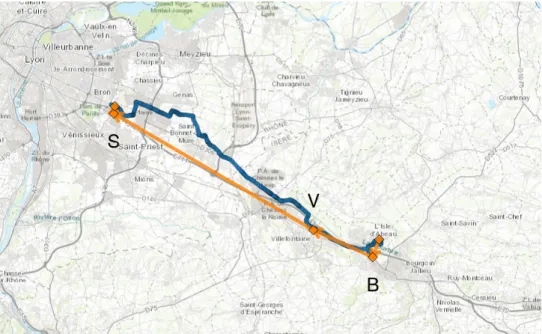
A complete GPS trace X is displayed as the sequence of 530 blue circles in Figure7. This GPS trace passes within 1 km of the B, V and S meeting point nodes, so its simplified topology consists of the 5-node sequence {origin > B > V > S > destination}, shown as the orange arrows. This simplified GPS trace represents a data compression rate of over 99% yet it retains the important information to decide the matching potential of this GPS driver trace with a passenger request on the Bourgoin > St-Priest carpooling line. In Table 2is the average data compression for the ˜n = 121 GPS traces on the Bourgoin > St-Priest line. The first column is the average number of GPS points in the complete driver traces #X, the second is the average number of GPS points of the simplified topologies # ˜X, and the last column is the average data compression rate (1 − # ˜X/#X).
Line # points in complete GPS traces
# points in simplified
GPS traces % compression
B > S 313 5 98.3
Table 2: Data compression rate on the Bourgoin > St-Priest carpooling line, during the morning operating hours 06:30–09:00, for all driver GPS traces from 2019-07-25 to 2020-02-17. The first column is the average number of GPS points in the complete driver traces, the second is the average number of points of the simplified GPS traces, and the third column is the average data compression rate.
4.2 Driver flow estimation
Of the ˜n = 121 GPS traces that follow the Bourgoin > St-Priest carpooling line, 31 GPS traces have an arrival time at Bourgoin within 08:00 to 08:30, i.e., a close spatio-temporal match for a passenger request for a departure at the Bourgoin meeting point between 08:00 and 08:30 am,
Figure 7: Topological simplification of a GPS trace in the Bourgoin > St-Priest carpooling line, during its morning operating hours 06:30–09:00, on 2019-11-28. The complete GPS trace are the 530 blue circles; the sequence of five nodes, as its simplified topology, are the orange arrows, and the orange diamonds are the origin, carpooling meeting points, destination nodes. The meeting points are S = St-Priest, V = Villefontaine, and B = Bourgoin.
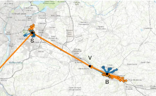
with a destination at the St-Priest meeting point. Of these 31 GPS traces, 17 of them are door-to-door matches (as defined as belonging to the largest door-door-to-door cluster of GPS traces in Table 1). These 17 traces are both door-to-door and meeting point matches and their simplified traces are displayed in Figure 8 as the orange diamonds/arrows. The simplified traces of the remaining 14 meeting point but not door-to-door matches are the blue diamonds/arrows. The latter represent an 82% increase in the number of drivers (from 17 to 31) who can potentially respond to a passenger carpooling request on the Bourgoin > St-Priest line.
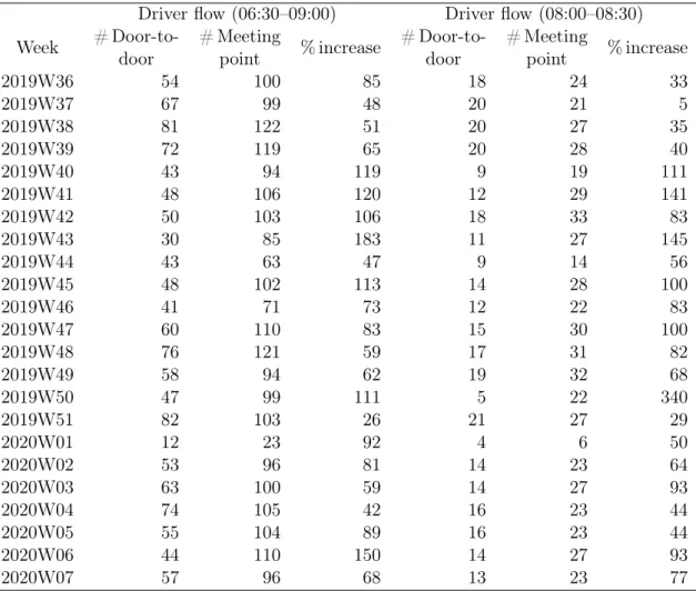
Table 3 summarises the weekly evolution of the impact of meeting point matching over door-to-door matching. The first set of three columns focus on the entire morning operat-ing hours (06:30–09:00) whereas the second set on the soperat-ingle 30 minute period (08:00–08:30) as this latter restricted period is a more realistic time frame that potential passengers are willing to wait for a driver to arrive. The first column contains the weekly aggregate num-ber of door-to-door matches, the second the numnum-ber of meeting point matches, and the third is the percentage increase due to meeting point matches, i.e. (# meeting point matches − # door-to-door matches)/# door-to-door matches. The number of door-to-door matches are enu-merated from a similar hierarchical clustering to that in Table 1, and the number of meeting point matches are computed from Equation (1). This table demonstrates that the increase in the driver flow due to meeting point matching is maintained over the entire data collection period.
The simplified GPS traces also allow us to compute the driver flows for narrower time intervals than the 2.5 hour and 0.5 hour intervals in Table 3. FollowingSmith and Demetsky [1997] and McShane and Roess[1990] that 15 minutes intervals are a suitable choice because the variation in driver flows for shorter intervals is less stable, Table 4 displays the average driver flow for 15 minute intervals during 06:30 to 09:00. For robustness, we aggregate these driver flows over all
Figure 8: Matching on meeting points increases the number of driver spatio-temporal matches in comparison to door-to-door matching, during a single 30 minute period (08:00-08:30), on 2019-11-28. The orange arrows are the 14 GPS traces which are both meeting point and door-to-door, and the blue arrows are the 17 GPS traces which are meeting point matches but not door-to-door match matches. The diamonds are the origin/destination points. The solid black circles are the meeting points: S = St-Priest, V = Villefontaine, and B = Bourgoin.
weeks in the data collection period in applying Equation (1) since we have increased the intra-day temporal resolution.
4.3 Waiting time prediction
It is straightforward to convert these average driver flows in Table4into predicted waiting times using Equation (2). Suppose that a passenger makes a carpool request at 08:10 at the Bourgoin meeting point to travel to St-Priest. The expected waiting time is the length of the interval divided by the average driver flow in the interval 08:00–08:15, i.e. 7.5 minutes. Given that we have already established a highly detailed spatio-temporal profile of the average driver flow for a carpooling line in Table 4, then the predicted waiting times at the same temporal resolution are shown in Table 5.
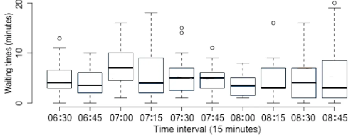
For the Bourgoin > St-Priest carpooling line from 2019-07-25 to 2020-02-17, we observed roughly 1500 carpooling requests with a reliably recorded waiting time. Each box plot in Figure9 displays the observed waiting times each 15 minute interval during the morning opening hours with at least one observed waiting time.
The accuracy of these predicted waiting times with respect to these observed ones is illustrated in Figure10. Each box plot displays the RMSE (Root Mean Squared Error) between the observed and the predicted waiting times (from Table 5) for each 15 minute interval. For all 15 minute intervals, the median RMSE is around 2 to 4 minutes which implies that the predicted waiting times fairly closely track the observed waiting times. This gives us confidence in our method for predicting waiting times in a stochastic carpooling service.
Driver flow (06:30–09:00) Driver flow (08:00–08:30) Week # Door-to-door # Meeting point % increase # Door-to-door # Meeting point % increase 2019W36 54 100 85 18 24 33 2019W37 67 99 48 20 21 5 2019W38 81 122 51 20 27 35 2019W39 72 119 65 20 28 40 2019W40 43 94 119 9 19 111 2019W41 48 106 120 12 29 141 2019W42 50 103 106 18 33 83 2019W43 30 85 183 11 27 145 2019W44 43 63 47 9 14 56 2019W45 48 102 113 14 28 100 2019W46 41 71 73 12 22 83 2019W47 60 110 83 15 30 100 2019W48 76 121 59 17 31 82 2019W49 58 94 62 19 32 68 2019W50 47 99 111 5 22 340 2019W51 82 103 26 21 27 29 2020W01 12 23 92 4 6 50 2020W02 53 96 81 14 23 64 2020W03 63 100 59 14 27 93 2020W04 74 105 42 16 23 44 2020W05 55 104 89 16 23 44 2020W06 44 110 150 14 27 93 2020W07 57 96 68 13 23 77
Table 3: Weekly aggregate driver flow increase of meeting point matching compared to door-to-door matching in the Bourgoin > St-Priest carpooling line, during the morning operating hours 06:30–09:00, and 08:00–08:30, from 2019-09-02 to 2020-02-17. The first columns contains the number of door-to-door matches, the second the number of meeting point matches, and the third the percentage increase due to the meeting point matches.
Driver flow Line 06:30 –06:45 06:45 –07:00 07:00 –07:15 07:15 –07:30 07:30 –07:45 07:45 –08:00 08:00 –08:45 08:15 –08:30 08:30 –08:45 08:45 –09:00 B > S 1 1.5 2.5 1.5 3 1.5 2 2 2 1
Table 4: Daily average driver flow on the Bourgoin > St-Priest carpooling line, per 15 minute intervals, during the morning operating hours 06:30–09:00 for a typical day from 2019-09-02 to 2020-02-17.
Since there is no comparable operational door-to-door carpooling service to Bourgoin > St-Priest stochastic carpooling line, then it is not possible to compare empirical waiting times from each type of carpooling. Our proxy is to compare the predicted waiting times for the door-to-door matches and the meeting point matches. Since our method for waiting time prediction is
Predicted waiting time (min) Line 06:30 –06:45 06:45 –07:00 07:00 –07:15 07:15 –07:30 07:30 –07:45 07:45 –08:00 08:00 –08:45 08:15 –08:30 08:30 –08:45 08:45 –09:00 B > S 15.0 10.0 6.0 10 6.0 5.0 7.5 7.5 7.5 15
Table 5: Waiting time predictions for a carpool request on the Bourgoin > St-Priest carpooling line, per 15 minute intervals, during the morning operating hours 06:30–09:00 for a typical day from 2019-09-02 to 2020-02-17.
Figure 9: Box plots of observed waiting times on the Bourgoin > St-Priest carpooling line, per 15 minute intervals during the morning operating hours 06:30–09:00, from 2019-09-02 to 2020-02-17.
Figure 10: RMSE between the observed and predicted waiting times on the Bourgoin > St-Priest carpooling line, per 15 minute intervals during the morning operating hours 06:30–09:00, from 2019-09-02 to 2020-02-17.
fairly accurate for meeting point matches according to Figure10, we reason that it will also yield accurate waiting times for door-to-door matches. In Table6are the predicted waiting times based on the weekly aggregate driver flows from Table 3 via Equation (2) for both door-to-door and meeting point matches. For all weeks, we observe a decrease in the predicted passenger waiting
times. From anecdotal evidence from Ecov, 15 minutes corresponds roughly to the maximum time that passengers are willing to wait for a driver to arrive since a pre-arranged meeting time has not made. This 15 minute threshold is exceeded by the door-to-door waiting times for most weeks, whereas the meeting point matched waiting times are lower than 15 minutes for most weeks.
Predicted waiting time (06:30–09:00) Predicted waiting time (08:00–08:30)
Week
Door-to-door (min)
Meeting
point (min) % decrease
Door-to-door (min)
Meeting
point (min) % decrease
2019W36 13.9 7.5 –46 8.3 6.2 –25 2019W37 11.2 7.6 –32 7.5 7.1 –5 2019W38 9.3 6.1 –34 7.5 5.6 –26 2019W39 10.4 6.3 –39 7.5 5.4 –29 2019W40 17.4 8.0 –54 16.7 7.9 –53 2019W41 15.6 7.1 –55 12.5 5.2 –59 2019W42 15.0 7.3 –51 8.3 4.5 –45 2019W43 25.0 8.8 –65 13.6 5.6 –59 2019W44 17.4 11.9 –32 16.7 10.7 –36 2019W45 15.6 7.4 –53 10.7 5.4 –50 2019W46 18.3 10.6 –42 12.5 6.8 –45 2019W47 12.5 6.8 –45 10.0 5.0 –50 2019W48 9.9 6.2 –37 8.8 4.8 –45 2019W49 12.9 8.0 –38 7.9 4.7 –41 2019W50 16.0 7.6 –53 30.0 6.8 –77 2019W51 9.1 7.3 –20 7.1 5.6 –22 2020W01 14.2 7.8 –45 10.7 6.5 –39 2020W02 11.9 7.5 –37 10.7 5.6 –48 2020W03 10.1 7.1 –30 9.4 6.5 –30 2020W04 13.6 7.2 –47 9.4 6.5 –30 2020W05 17.0 6.8 –60 10.7 5.6 –48 2020W06 13.2 7.8 –41 11.5 6.5 –43 2020W07 53.6 41.7 –22 30.0 30.0 0
Table 6: Weekly predicted passenger waiting times for door-to-door and meeting point matching in the Bourgoin > St-Priest carpooling line, during the morning operating hours 06:30–09:00, and 08:00–08:30, from 2019-09-02 to 2020-02-17. The first columns contains the predicted wait-ing times for door-to-door matches, the second for meetwait-ing point matches, and the third the percentage decrease due to the meeting point matches.
4.4 Driver participation rate estimation
A key question for the service provider is what driver participation rate leads to passenger waiting times around 5 to 10 minutes, as observed in Figure 9? To respond to this question, we first need to enumerate the population of all drivers on a carpooling line. The county-level origin-destination matrix of home-work trajectories from the French official statistical agency [INSEE, 2018] is insufficiently detailed to decide if the drivers with these origins-destinations travel on the carpooling lines. So we infer likely trajectories, as determined as the fastest route by the
TomTom route finder API [TomTom, 2019] starting on Tuesday 8am from the origins (county centroids) to the destinations (county centroids). A spatial intersection, similar to that carried out for the driver GPS traces, is computed to determine which trajectories pass within 1 km of the carpooling meeting points. These trajectories are shown in Figure11. Note that there is no temporal information attached to this origin-destination matrix, but since they are home-work trajectories, we suppose they are effected in the morning peak hours which matches the time interval of the driver GPS traces.
Figure 11: Likely driver itineraries from the TomTom route finder API in the same geographical region as the Bourgoin > St-Priest carpooling line. The origins and destinations (county cen-troids) are the orange diamonds. The solid black circles are the meeting points: S = St-Priest, B = Bourgoin.
If we then aggregate the corresponding driver flows in the origin-destination matrix, then we obtain ˜n0 = 3821 drivers whose likely trajectories match the Bourgoin > St-Priest carpooling line.
From Table4, there is a daily average of ˜n = 20 driver GPS traces between 06:30 and 09:30. This yields an estimated driver participation rate of ˜P = ˜n/˜n0 = 0.52% from Equation (3). Even with
this low driver participation rate, average passenger waiting times of 5–10 minutes are observed in Figure 9.
If we were able to increase this low driver participation rate even modestly (to 1% or 5%), then the predicted passenger waiting times would fall substantially, as illustrated in Figure 12. In this case, these waiting times would be lower than those of bus lines and approach those of high frequency metro/subway train lines. The methods for increasing driver participation, as they lie largely outside of data science, are out of scope of this paper but are of intense interest to the service provider [Zhu,2017,2018,2020].
5
Conclusions and future work
Stochastic real-time carpooling services differ from competing services which offer deterministic door-to-door matching for complete trajectories. Whilst the latter offer a high level of personal
Figure 12: Evolution of the predicted passenger waiting time as a function of the driver par-ticipation rate in the Bourgoin > St-Priest carpooling line, during the morning operating hours 06:30–09:00, from 2019-07-25 to 2020-02-17.
convenience in highly urbanised regions, door-to-door matching structurally inhibits mass adop-tion of carpooling, especially in peri-urban regions. Relaxing the strict door-to-door matching allows, and subsequently implementing stochastic meeting point matching, allows for the mutu-alisation of high throughput road segments, and thus removes this obstacle. We introduced a novel data science-GIS workflow for a stochastic carpooling service. The crucial mathematical abstraction in this workflow is to reduce the complexity of driver GPS traces to a graph-based topology of the carpooling network. We illustrated this workflow on an operational stochastic carpooling service in a peri-urban region in south-eastern France. We provided quantitative justi-fications that the physical meeting points, by facilitating a critical mass of drivers and passengers drawn from a much larger geographical area, leads to passenger waiting times which are lower than those achieved by door-to-door matching. Our workflow is novel combination of two closely related, but historically separate, disciplines of data science and GIS into a single workflow. In addition to predicting the passenger waiting times, it is able to deliver outputs for the driver flow maps, driver flow spatio-temporal profiles, and driver participation rates. This workflow forms a solid prototype for other workflows to accompany the expansion of stochastic carpooling services to address the mobility requirements in neglected peri-urban regions in the future.
6
Acknowledgements
The authors thank Ecov for providing the data sets of driver GPS traces and passenger waiting times. The authors also thank Bertrand Michel from the Central Engineering School of Nantes and Gérard Biau from Sorbonne University for their feedback.
References
Carol Cooper. Successfully changing individual travel behavior: Applying community-based social marketing to travel choice. Transportation Research Record, 2021:89–99, 2007.
Required to Represent a Digitized Line or its Caricature. Classics in Cartography: Reflections on Influential Articles from Cartographica, 10:15–28, 2011. doi: 10.1002/9780470669488.ch2.
Masabumi Furuhata, Maged Dessouky, Fernando Ordóñez, Marc-Etienne Brunet, Xiaoqing Wang, and Sven Koenig. Ridesharing: The state-of-the-art and future directions. Trans-portation Research Part B: Methodological, 57:28–46, 2013.
Keivan Ghoseiri. Dynamic Rideshare Optimized Matching Problem. PhD thesis, University of Maryland, 2012.
Riccardo Guidotti, Mirco Nanni, Salvatore Rinzivillo, Dino Pedreschi, and Fosca Giannotti. Never drive alone: boosting carpooling with network analysis. Information Systems, 64:237– 257, 2017.
INSEE. Mobilités professionnelles en 2015: déplacements domicile–lieu de travail. National Institute of Statistics and Economic Studies [INSEE], France., 2018. In French.https://www. insee.fr/fr/statistiques/3566477.
Dong Woo Lee and Steve H. L. Liang. Crowd-sourced carpool recommendation based on simple and efficient trajectory grouping. In Proceedings of the 4th ACM SIGSPATIAL International Workshop on Computational Transportation Science, pages 12–17, 2011. doi: 10.1145/2068984. 2068987.
Xin Li, Sangen Hu, Wenbo Fan, and Kai Deng. Modeling an enhanced ridesharing system with meet points and time windows. PLOS ONE, 13:1–19, 2018.
William R McShane and Roger P Roess. Traffic Engineering. Prentice-Hall, 1990.
OpenStreetMap contributors. OpenStreetMap. https://www.openstreetmap.osm, 2019.
Susan A. Shaheen, Nelson D. Chan, and Teresa Gaynor. Casual carpooling in the San Francisco Bay Area: Understanding user characteristics, behaviors, and motivations. Transport Policy, 51:165 – 173, 2016.
Susan A. Shaheen, Adam Stocker, and Marie Mundler. Online and app-based carpooling in France: Analyzing users and practices – a study of BlaBlaCar. In Gereon Meyer and Susan Shaheen, editors, Disrupting Mobility: Impacts of Sharing Economy and Innovative Trans-portation on Cities, pages 181–196. Springer International Publishing, 2017.
Brian L Smith and Michael J Demetsky. Traffic flow forecasting: comparison of modeling ap-proaches. Journal of Transportation Engineering, 123:261–266, 1997.
Mitja Stiglic, Niels Agatz, Martin Savelsbergh, and Mirko Gradisar. The benefits of meeting points in ride-sharing systems. Transportation Research Part B: Methodological, 82:36–53, 2015.
Jinjin Tang, Ying Song, Harvey J. Miller, and Xuesong Zhou. Estimating the most likely space–time paths, dwell times and path uncertainties from vehicle trajectory data: A time geographic method. Transportation Research Part C: Emerging Technologies, 66:176 – 194, 2016.
TomTom. Routing API and Extended Routing API, 2019. https://developer.tomtom.com/ routing-api.
Hai Wang and Hai Yang. Ridesourcing systems: A framework and review. Transportation Research Part B: Methodological, 129:122–155, 2019.
Dianzhuo Zhu. More generous for small favour? Exploring the role of monetary and pro-social incentives of daily ride sharing using a field experiment in rural Île-de-France. DigiWorld Economic Journal, 108:77–97, 2017.
Dianzhuo Zhu. The limit of money in daily ridesharing: Evidence from a field experiment. Technical report, PSL, University of Paris-Dauphine, 2018.
Dianzhuo Zhu. Understanding Motivations and Impacts of Ridesharing: Three Essays on Two French Ridesharing Platforms. PhD thesis, PSL, University of Paris-Dauphine, 2020.