Development and biodiversity conservation in Sub-Saharan Africa: A spatial analysis

HAL Id: halshs-00799175

https://halshs.archives-ouvertes.fr/halshs-00799175

HAL is a multi-disciplinary open access archive for the deposit and dissemination of sci-entific research documents, whether they are pub-lished or not. The documents may come from teaching and research institutions in France or abroad, or from public or private research centers.

L’archive ouverte pluridisciplinaire HAL, est destinée au dépôt et à la diffusion de documents scientifiques de niveau recherche, publiés ou non, émanant des établissements d’enseignement et de recherche français ou étrangers, des laboratoires publics ou privés.

Sub-Saharan Africa: A spatial analysis

Ariane Manuela Amin, Johanna Choumert

To cite this version:

Ariane Manuela Amin, Johanna Choumert. Development and biodiversity conservation in Sub-Saharan Africa: A spatial analysis. 2013. �halshs-00799175�

C E N T R E D'E T U D E S E T D E R E C H E R C H E S S U R L E D E V E L O P P E M E N T I N T E R N A T I O N A L

SERIE ETUDES ET DOCUMENTS DU CERDI

Development and biodiversity conservation in Sub-Saharan Africa:

A spatial analysis

Ariane AMIN, Johanna CHOUMERT

Etudes et Documents

_{n° 02}

March 2013

CERDI

65 BD. F. MITTERRAND

63000 CLERMONT FERRAND – FRANCE TEL. 0473177400

FAX 0473177428

2 The authors

Ariane AMIN

PhD student, Clermont Université, Université d'Auvergne, CNRS, UMR 6587, CERDI, F-63009 Clermont Fd

Email: Ariane_Manuela.Amin@etu.udamail.fr Johanna CHOUMERT

Associate Professeur, Clermont Université, Université d'Auvergne, CNRS, UMR 6587, CERDI, F-63009 Clermont Fd

Email: Johanna.choumert@udamail.fr

La série des Etudes et Documents du CERDI est consultable sur le site :

http://www.cerdi.org/ed

Directeur de la publication : Patrick Plane

Directeur de la rédaction : Catherine Araujo Bonjean Responsable d’édition : Annie Cohade

ISSN : 2114 - 7957

Avertissement :

Les commentaires et analyses développés n’engagent que leurs auteurs qui restent seuls responsables des erreurs et insuffisances.

3 Abstract

A better understanding of the relationship between economic development and biodiversity loss is of great relevance, given the current rapid extinction of species along with challenges born from the context of economic development in poor countries. The purpose of the current study is to provide a sound analysis, within the framework of an Environmental Kuznets Curve, of the relationship between economic development and pressure on biodiversity. Drawing on the most up-to-date data on threatened species from 48 sub-Saharan African countries, we used Maximum-likelihood and generalized spatial two-stage least-squares estimators to account for spatial-autoregressiveness in the dependent variable, as well as in the explanatory variables and in the disturbances of the models. We find evidence that supports an inverted U-shaped relationship between development and biodiversity imperilment, measured as the percent of threatened bird species. The results also reveal some species-level differences in the biodiversity-development relationship, since the Environmental Kuznets Curve hypothesis doesn’t hold for mammals. This analysis contributes to the literature by partially challenging the paradigm of a strictly negative relationship between biodiversity and development in a developing countries context.

Keywords: Biodiversity, species imperilment, spatial econometrics, Cliff-Ord model, spatial

Durbin model

4

1 Introduction

The XI/22 decisions of the Convention on Biological Diversity –CBD– at its eleventh Conference of Parties invites parties to integrate the three objectives of the CBD into sustainable development and poverty eradication programs, plans, policies, and priority actions, taking into account the outcomes of the Rio+20 Conference (UNEP, 2012). Target 2 of strategic goal A of the Aichi Biodiversity Target, in the same vein, recommends that by 2020, at the latest, biodiversity values have been integrated into national and local development and poverty reduction strategies and planning processes and are being incorporated into national accounting, as appropriate, and reporting systems (UNEP, 2010). The link between biodiversity, poverty eradication and development, which had been treated as separate issues, is now widely accepted and appears explicitly in international agendas.

The widespread acceptance of this link is justified since biodiversity and the many ecosystem services that it provides are a key factor determining human wellbeing (MEA, 2005). Moreover, biodiversity loss has direct and indirect negative effects on several factors such as food security, vulnerability, health, energy security, clean water, social relations, and basic materials (MEA, 2005), which are also essential for economic and human development. Competing development goals, such as food production, however, contribute to accelerate erosion of biodiversity, to the extent that our natural stock of capital is being reduced (TEEB, 2009).

The depletion of biodiversity is now one of the most important environmental threats that humanity faces (Chapin et al., 2000; Tilman, 2000; MEA, 2005). Regarding the consequences of biodiversity loss however, not all people are impacted equally. Changes in ecosystems disproportionately harm many of the world's poorest people, who are less able to adjust to these changes and who are affected by even greater poverty, as they have limited access to substitutes or alternatives (MEA, 2005). The less developed regions in the world, where the poorest people, most vulnerable to biodiversity loss, live, are also regions where threats to biodiversity are the highest (Du castel, 2007). The Sub-Saharan Africa –SSA– region is a good illustration of such a developing region that is at the forefront of priorities in terms of conservation as well as development needs (cf. Figure 1 in Appendix A). Indeed, the SSA region ranks first in terms of highest and relatively steady poverty rate since 1981 according to World Bank reports (Haughton and Khandker, 2009). The SSA region is home to also almost one-quarter of the “biodiversity hotspots”, i.e. areas around the world where

5 exceptional concentrations of endemic species are undergoing exceptional loss of habitat (Myers et al, 2000).

Despite the fact that the CBD decisions and Aichi targets recommend moving forward with integrated strategies, practically speaking, policies that tackle conservation and development issues together are not likely to be implemented any time soon. Furthermore, we suppose that the consideration of these pro-conservation recommendations does not affect, for the meantime and especially in developing areas, the on-going development strategies whether they are incentives or disincentives for biodiversity conservation. Given the importance of biodiversity in the transition to integrated strategies, it is important to discuss further whether tireless efforts to meet development and poverty reduction will not lastingly compromise biodiversity. The problematic is especially of great relevance, in areas where biodiversity depletion is already an issue of great concern. In others words, since we need to deal with development and poverty challenges – for a region like SSA which is also a “biodiversity hotspot”– shall we be optimistic or pessimistic about biodiversity and the maintenance of related local and global environmental services?

The matter of whether economic development worsens or strengthens biodiversity conservation has been overlooked in the literature. A number of researchers share a pessimistic view and forecast a conflict between economic growth and biodiversity conservation (Chambers et al., 2000; Czech, 2003; Trauger et al., 2003). They suggest that increased growth of the economy implies higher threats to biodiversity (Asafu-Adjaye, 2003; Freytag et al., 2009). Other scholars, more optimistically, reject the monotonic relationship assumption and argue that the relationship between economic growth and biodiversity conservation varies along the development path. They predict a “virtuous circle” after a threshold of development is reached, thus implying an environmental Kuznets curve for biodiversity (Naidoo and Adamowicz, 2001; McPherson and Nieswiadomy, 2005; Pandit and Laband, 2007; Mills and Waite, 2009). The logic is that when enough financial wealth accumulates, especially in per capita terms, society refocuses on solving environmental problems (Czech, 2008). As we can see, empirical findings have not yet provided a clear-cut answer to the question of the impact of economic development on pressure on biodiversity, even less for a specific geographical area. In this paper, we propose further investigation on the issue and provide a sound analysis for the specific area of the SSA region.

6 We suggest that the current rapid loss of biodiversity will decrease once a certain economic level is reached in SSA, indicating the existence of an EKC. Following McPherson and Nieswiadomy (2005) regarding the existence of spillover effects into surrounding countries for biodiversity loss, we control for spatial autocorrelation in models. Regarding the concerns of our study, i.e. threats to biodiversity, there may be several sources of spatial dependence in data and therefore different possible spatial specifications. First, national policies for conservation of biodiversity may be influenced by policies in neighboring countries, resulting in a pattern of political spatial dependence. This can be modeled through a spatial lag model – LAG– (or first-order spatial auto-regression model–SAR (1)). Second, there may be spillovers between countries. For example, if a country introduces regional or national policies to promote biodiversity, this can have positive effects in neighboring countries, since species (like birds or mammals) are mobile and– if noteworthy to say – do not respect political boundaries. This can be tested through a spatial lag model. Third, unobserved variables may be related by a spatial process, such as climate variables. In this case, a spatial error model – SEM model- is to be estimated. As there is no theoretical argument to choose or exclude a specification a priori, we test a Cliff-Ord model (also known as Kelejian-Prucha model), that enable us to test for the simultaneous presence of spatial lag and spatial error in data or the presence of one or the other. In this way, our paper is the first to consider a Cliff-Ord model in biodiversity Kuznets curve framework. We go further by also addressing the critiques of Elhorst (2010) and Corrado and Fingleton (2011), who noted that evidence of spatial dependence, is likely to capture the omission of spatially correlated omitted variables. In response, we test a model that includes spillovers associated with first order spatial autoregression and spatially lagged explanatory variables, called the Spatial Durbin Model (SDM model).

The argument proceeds in four parts. First, we examine BKC investigation in the literature and from this identify methodological striking points that we consider to improve our empirical approach. Second, we describe our methodology and modeling techniques. Thereafter, we analyze the data and discuss our results, while the final section concludes and shows how our findings can inform policymakers.

2 Biodiversity Kuznets Curve: Mains findings and methodological issues

The first empirical environmental Kuznets curve—EKC—studies appeared independently in three working papers: Grossman and Krueger (1991); Shafik and

7 Bandyopadhyay (1992); and Panayotou (1993) (cf.Dinda, 2004). In these seminal papers, environmental degradation is predicted to increase with growing income up to a turning point, beyond which environmental quality improves with higher income per capita. A large body of literature has investigated the EKC theory after these first works, and substantial evidence supporting the EKC has been provided for various types of environmental damage, such as air pollution (Grossman and Krueger,1991; Kearsley and Riddel, 2010), water pollution (Shafik, 1994; Heerink et al., 2001), and deforestation (Bhattarai and Hammig, 2001; Culas, 2007). Stern (2004) and Dinda (2004) provide thorough surveys. More recently, a number of studies have dealt with the possibility to expand the EKC theory to biodiversity loss (Naidoo and Adamowicz, 2001; McPherson and Nieswiadomy, 2005; Pandit and Laband, 2007; Mills and Waite, 2009). They examine whether the threat to biodiversity appears to rise up to a certain level of per capita income and thereafter decline. These investigations, i.e. research on empirical evidence for a biodiversity Kuznets curve—BKC hereafter—face a lot of challenging methodological issues. The first is related to the choice of biodiversity indicator, the second to the shape of the BKC, the third to spatial autocorrelation in data.

2.1 On the choice of biodiversity indicator

Studies of how development path affects biodiversity run into difficulties in appraising biodiversity erosion. We do know that a precise measurement of environmental damage is important in studying the EKC whose aim is to describe a general relationship between the economy and the environment (Bagliani et al, 2008). For the concern of BKC specifically, should the threat to biodiversity be measured as a threat to particular species, ecosystem,

genes, or as a threat to overall biodiversity? Part of the answer will depend on theoretical

arguments that could support the empirical evidence for a BKC. According to Naidoo and Adamowicz (2001), the rising then falling threat to biodiversity along the development path is a result of the interaction of income elasticity, institutional design, and biological characteristics. The rise of income per capita would result in a higher demand for species protection, for example, that would induce policy responses, manifested by more stringent biodiversity conservation policies. To the extent that individual preferences may be expressed, it is likely that the link between income and species will vary by taxonomic group. As evidence, diverse studies show that conservation efforts have been motivated less by the degree of threat and more by whether the species belong to a particular charismatic taxonomic group (Simon et al.1995; Metrick and Weitzman 1996, 1998; Dawson and Shogren, 2001; Mahoney, 2009). Furthermore, according to Czech et al. (1998), some taxa (birds and

8 mammals) are particularly advantaged in terms of both their social construction and the amount of political power endowed to them by various conservation groups. Following these arguments, biodiversity should not be considered as a whole in the biodiversity-development relationship. Yet for some authors, studies that do so, such as those that use data on specific species as biodiversity indicators, do not account for variations in ecosystems which directly affect species diversity. They do not include the overall risk of biodiversity loss that includes risk to genetic as well as ecosystem diversity (Mozumder et al., 2006).

Regarding empirical findings, robust evidence for a BKC has been found when using threatened birds as an indicator (Naidoo and Adamowicz, 2001; McPherson and Nieswiadomy, 2005; Pandit and Laband, 2007). Hence, there is an inverted U-shaped relationship between the ratio of threatened birds and per capita income levels, although empirical explanation is not clearly developed in the literature. The existence of an inverted U relationship is not compelling for other taxa. Studies using a multidimensional or global indicator such as the National Biodiversity Risk assessment Index (NABRAI) (Mozumder et al., 2007) or species richness (Dietz and Adger, 2003) do not support, in general, an EKC relationship for biodiversity. This likely reveals the ambiguousness of a global indicator for a BKC investigation and tends to support a taxa-level indicator.

2.2 On the shape of the BKC

Another important sticking point in the literature on BKC is the shape of the curve. A U-shaped curve admits the expectation to see a “rising limb” at higher income levels, assuming, for instance, an increase in species diversity of the same magnitude of their erosion. Because the process by which species become extinct proceeds markedly more rapidly than that by which new species are created (Schubert and Dietz, 2001), such replenishment of species diversity at the same rate of their loss seems impossible. It is therefore proposed that, instead of a quadratic shape, the BKC may be modeled as a hyperbolic curve which combines the “falling limb” of the EKC and a slowing of biodiversity loss (Schubert and Dietz, 2001). The hyperbolic BKC postulates that structural changes or income elasticity of demand for biodiversity cannot reverse the impact of development acceleration on biodiversity loss. Even if the irreversibility of the relationship is comprehensive, due to ecological thresholds (Dasgupta, 2000) and the unique nature of the damage (e.g., loss of critical habitat and keystone species), a BKC is theoretically possible, albeit perhaps very difficult to achieve (Mills and Waite, 2009). Schubert and Dietz (2001) have tested a linear, quadratic, and

9 hyperbolic functional form, for species richness and GDP per capita. They found that the quadratic form has no better fit than the others but failed to empirically identify the best shape for the relation between income and biodiversity. Dietz and Adger (2003) also failed to provide evidence to justify preference for a hyperbolic BKC. Mills and Waite (2009) notice that Dietz and Adger (2003) inadvertently obscure a parabolic relationship by the way they graphed their data. They find, extending the work of Dietz and Adger (2003), that the simple parabolic model is significant and better than linear and hyperbolic models.

2.3 Spatial interactions

A recent development in the EKC literature especially, which is focused on biodiversity, is the incorporation of spatial information to account for spatial autocorrelation. Although geographical areas (or cross-sectional units) form the basic unit of analysis in most EKC studies, virtually all have ignored underlying spatial relationships among units (Rupasingha et al., 2004). Ignoring spatial dependence leads to model misspecification (Anselin, 1988) and accounting for transboundary influences could significantly alter the perceived shape of the EKC (Maddison, 2006). Concerning biodiversity, spatial autocorrelation is a typical problem (Kerr and Burkey, 2002). Indeed, the distribution of plants and animal species is determined by geophysical, atmospheric, and ecological factors that cut across political jurisdictions (Pandit and Laband, 2007). Consequently, factors that influence biodiversity threats may extend or operate beyond arbitrary political boundaries and risks to biodiversity in one country may similarly impact biodiversity in neighboring countries through spillover effects. McPherson and Nieswiadomy (2005) were the first to consider the problems surrounding spatial autocorrelation, investigating the EKC for threatened species. While they find evidence for both spatial error dependence and spatial lag in the data, corroborating the presence of positive spatial dependency, they only report results for the spatial lag model. Pandit and Laband (2007), however, establish that spatial error models result in greater explanatory power than spatial lag models for mammals, birds, amphibians, and vascular plants. Regarding the impact of spatial information on BKC findings, Pandit and Laband (2007) notice that spatial dependence affects their results only for mammals and amphibians. Mills and Waite (2009) on the contrary, find that the inclusion of the spatial covariates does not change the results or the direction of any of their previous models on BKC with species richness as the biodiversity indicator.

Spatial econometrics encounters a lot of skeptics, due to the fact that the spatial autocorrelation in the dependent variable is often significant (Corrado and Fingleton, 2011).

10 As noted by Corrado and Fingleton (2011), this is likely due to the omission of spatially correlated omitted variables. In addition, the choice of the relevant spatial model is another sticking point in spatial analysis. No study to date on a spatial BKC has taken into consideration the existence of both spatial error dependence and spatial lag in the data, although it is possible. There is also a lack of analysis which tries to investigate, beyond the information that biodiversity loss in one country is significantly influenced by adjacent countries, which specific aspects of those adjacent countries affect biodiversity in the referent country.

3 Empirical analysis

In view of the literature review in part 2, our analysis will focus around the following points. First, we will use specific taxa data and not aggregated data for biodiversity. Second, we will test a hyperbolic BKC and a quadratic BKC. Finally, we will focus on improving the spatial analysis, a necessary step in providing robust evidence for the development-biodiversity link.

3.1 Data

We aim to discover biodiversity trends along the development path in some specific developing areas, where biodiversity is already deteriorating and where there is an irrepressible need for development and hence poverty reduction. When considering the combination of development and poverty reduction priorities along with biodiversity conservation ones, the SSA region ranks first. We decide then to focus on that region.

For measuring the pressure on biodiversity, we use the Percentage of Threatened Species (PTS) for birds and mammals at the country level for Sub-Saharan African countries. Birds and mammals species are the only taxonomic groups for which all species have been reviewed by the IUCN (Stattersfield and Capper, 2000; Hilton-Taylor, 2000). Hence we will estimate the model for two dependent variables, PTSBIRD and PTSMAM. We calculate the latter

for each taxon as the percentage of threatened species to known species in 2011 for mammals and in 2012 for birds.

Gross domestic product per capita (PCGDP) in constant 2005 US$, normalized for purchasing power, was used as an indicator of economic development. By adjusting for differences in cost of living and exchange rates between countries, gross domestic product in

11 purchasing power parity provides a better estimate of development and wellbeing in each country.

As control variables in the models, we select a spectrum of socio-economic and ecological characteristics of countries that are likely to have an influence on species imperilment. For socio-economic data, we use population density (per sq. km) at the country level (DENS), as Dietz and Adger (2003), Asafu-Adjaye (2003), and Pandit and Laband (2007). Following Kerr and Currie (1995), and Asafu-Adjaye (2003), we also employ, as a socio-economic variable, the percentage of agricultural land area (AGRI). We use as ecological variable, the percentage of endemism in birds (PESBIRD) and endemism in

mammals (PESMAM) in each country, as Naidoo and Adamowicz (2001), McPherson and

Nieswiadomy (2005), Pandit and Laband (2007), and Pandit and Laband (2009). The definition, interpretation, and source of data are given in Appendix B.

Table 1.Descriptive statistics

Variables Unit N Mean S.D. Min Max

PTSBIRDS % 48 3.63713 3.415438 .66335 15.29412

PTSMAM % 48 9.442919 5.814057 3.22581 31.57895

PCGDP

Constant 2005

US$ 48 2312.876 3266.579 333.6729 15196.24

PCGDP2 48 2.02e+07 5.63e+07 134586.4 2.72e+08

PCGDP-1 48 0.0011598 0.0007067 0.0003151 0.0040747

PESBIRDS % 48 2.86305 8.019604 0 43.9834

PESMAM % 48 4.167945 11.93176 0 80.08659

DENS hab./sq.km 48 76.62095 106.6808 2.325264 587.7394

AGRI % 48 47.93657 21.24915 8.244424 86.53946

We use averages of the explanatory variables for a period of 20 years (1992-2011), in line with McPherson and Nieswiadomy (2005). The intuition behind this procedure is to account for the fact that an indefinite span of time exists between anthropogenic factors and changes in biodiversity. This procedure also makes our study immune to short-term effects. The expected signs for the impact of our explanatory variables on the percentage of threatened species are presented in Appendix C. Our sample consists of 48 observations (Cf.

12 Appendix D for the list of countries present in the study). Table 1 presents descriptive statistics for all variables.

3.2 Spatial analysis

Assuming that spatial autocorrelation is a common problem for biodiversity data (Kerr and Burkey, 2002), we take into account spatial dependence and its magnitude among countries belonging to our sample. We look for evidence that the values for the percentage of threatened species of a taxon in Sub-Saharan African countries are more spatially clustered than they would be under random assignment. For this matter, we use spatial econometric techniques in order to include spatial relationships among observations (Anselin, 1988; Lesage and Pace, 2009). Spatial autocorrelation measures the intensity of the relationship between observations and their degree of resemblance. Each observation is described by one attribute (the dependent variable) and by proximity relations (weight matrices). If the presence of the attribute in one country makes its presence in a nearby country more or less likely, then there is spatial autocorrelation. There is no spatial autocorrelation if there is no relationship between the proximity of countries and their degree of resemblance. Spatial dependence may also arise from omitted variables which are spatially correlated, such as climatic conditions. Such an effect is called a spatial error. The latter can also be due to a wrong specification of the functional form or to measurement errors. Whatever the source of spatial dependence (spatial lag and/or spatial error), standard econometric techniques are no longer appropriate, especially the method of ordinary least squares. Instead, other estimators are proposed in the literature (see Anselin, 1988; Lesage and Pace, 2009; for further discussion on this topic).

3.2.1 Definition of neighborhood through spatial weight matrices

In spatial econometric models, neighborhood is defined exogenously, and this through weight matrices. A spatial weights matrix W is a matrix of dimension, N x N which brings together the neighborhood relations between observations, here countries. For instance, W12

gives the neighborhood relationship between country 1 and country 2. And self-neighbors are excluded (i.e. diagonal elements are equal to 0 or wii = 0).

We use two matrices. Matrix Wcijis based on 1st order contiguity, i.e. two countries are

neighbors if they share a common border such that:

wcij=1 if countries I and j share a common border

wcij=0 otherwise

According to Pandit and Laband (2007), such a matrix is more efficient than higher order adjacency, Euclidean distance between centroid points of adjoining countries, and percentage

13 of shared border. Next, following the idea proposed by McPherson and Nieswiadomy (2005), we construct the matrix WBij that contains the length of common borders between two

countries such that:

wBij=d

with d, the length of the border in km between country i and country j

Both weights matrices are row-standardized such as Σjwij = 1 for i = 1, …, n. In other words,

each element in row i is divided by the sum of i’s elements. Thus, lagged values will be averages of the variable at stake over the set of neighbors for each country i. Detailed information on matrices are given in Appendix B.

3.2.2 Econometric modeling

We adopt a specific-to-general approach. This step-by-step procedure enables comparative analysis between simple and spatial models. It is also useful to better capture the importance of considering spatial information in the analysis. We shall then start out with non-spatial BKC models. We test the two different functional forms proposed in BKC literature: quadratic and hyperbolic. Our basic regression model for the quadratic equation is:

PTSi= β0 + β1 PCGDPi + β2 PCGDPi2 + β3 DENSi+ β4 AGRIi+ β5 PESi+ ui. [1]

The hyperbolic equation is:

PTSi= β0 + β1PCGDPi-1 + β2 DENSi+ β3 AGRIi+ β4 PESi+ ui [2]

u~ N(0, σ2).

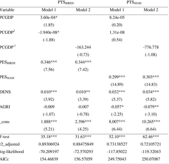
Table 2 presents the Huber-White sandwich estimator (Huber, 1967; White, 1980) and some scalar statistics for all models. The Huber-White sandwich estimator, or robust estimates of variance, gives estimates of the standard errors that are robust to the fact that the error term is not identically distributed. The overall explanatory power of the basic models is good for birds and mammals (see adjusted R2), which is confirmed by the fact that these models are statistically significant. Both the hyperbolic and linear equations fit the data significantly (see F-statistics) but the income terms are significant at the 1% level only for birds in quadratic equation. The corrected AIC score that is recommended to account for

14 small sample sizes (Burnham and Anderson, 2002), instead of AIC, is lowest for the quadratic equations (see AICc).According to the best model, as determined by R2, F test, t-test for GDP variables parameter, and AICc, the quadratic equation best fits our data. The remainder of this article will then focus on the quadratic equation for the BKC.

Table 2. Robust ordinary least square estimation of percent of threatened species (1992–2011 lagged averages of independent variables)

Biodiversity indicators

PTSBIRDS PTSMAM

Variable Model 1 Model 2 Model 1 Model 2

PCGDP 3.60e-04* 8.24e-05 (1.85) (0.20) PCGDP2 -1.940e-08* 1.31e-08 (-1.88) (0.54) PCGDP-1 -163.244 -776.778 (-0.73) (-1.08) PESBIRDS 0.346*** 0.344*** (7.56) (7.42) PESMAM 0.299*** 0.303*** (14.89) (14.83) DENS 0.010*** 0.010** 0.032*** 0.034*** (3.92) (3.39) (5.37) (5.82) AGRI -0.009 -0.007 -0.057* -0.079** (-1.07) (-0.78) (-2.25) (-3.10) _cons 1.888*** 2.396*** 8.007*** 10.265*** (5.21) (4.25) (6.44) (6.64) F-test 35.18*** 31.63*** 52.10*** 62.46*** r2_adjusted 0.89306924 0.88475849 0.73138527 0.72105721 log-likelihood -70.209197 -72.570293 -117.85022 -119.32043 AICc 154.46839 156.57059 249.75043 250.07087

N=48; *p<0.1;**p<0.05;***p<0.01 ;t-statistics are in parentheses

The tests for global spatial autocorrelation using Moran’s statistic (cf. Appendix E) show that the dependent variables PTSBIRD and PTSMAM exhibit positive and significant spatial

15 autocorrelation with all matrices used. For example, using the standardized weights matrix Wcij for the variable PTSBIRD, Moran’s I has a positive value equal to 0.546 with p-value equal

to 0. What is more, tests on regressions’ residuals indicate that the vector of disturbances exhibits spatial autocorrelation for PTSBIRD and PTSMAM in a multidirectional spatial model

that includes both the spatial lag term and a spatially correlated error structure (see robust LM test in Appendix F).

Given the fact that the spatial tests do not exclude a specification a priori, and indicate the simultaneous presence of an effect related to spatial spillovers in the endogenous variable and a spatial effect associated with spatially correlated errors, we turn then to a more sophisticated model capable of capturing all spatial effects. Kelejian and Prucha (1998, 1999) note that, researchers often estimate a spatial lag model or a spatial error model. It is commonly the case in the BKC literature that authors estimate a spatial lag model, or a spatial error model. Such a choice could be justified by theory, but often it is rather motivated by technical considerations. McPherson and Nieswiadomy (2005), in their seminal paper on a spatial BKC, state explicitly that they do not estimate a lag model and a spatial error model simultaneously for technical reasons. Contrary to previous works on a spatial BKC (McPherson and Nieswiadomy, 2005; Pandit and Laband, 2007; Pandit and Laband, 2009), we estimate a Cliff-Ord model that enables estimation of a spatial lag (first-order spatial autoregressive model) and a spatial error (spatial autoregressive structure for the disturbance) together, as suggested by Kelejian and Prucha (1998, 1999), such that:

PTSi = λ Σj#i wij PTSj + β0 + β1PCGDPi + β2 PCGDPi2 + β3 DENSi + β4 AGRIi+ β5 PESi+ ui,

ui = ρ Σj#i wijuj + εi, and ε~ N(0, σ2I).

λ reflects the magnitude of spatial dependence between observations. This spatial parameter measures the intensity of spatial interactions through the lagged dependent variable, i.e. the dependence of a country on nearby countries. ρ is a measure of spatial correlation in the errors. In this model, if λ=0, we would refer to a spatial error model; otherwise, if ρ =0 we would refer to a spatial lag model.

A priori, there is little guidance on the appropriate model. The spatial lag assumes that the pressure on birds in a country is influenced by the pressure on birds in neighboring countries via the parameter λ; ρ captures the effects of spatially correlated omitted variables.

16 We rely on a maximum likelihood (ML) estimator and a generalized spatial two-stage least-squares (GS2SLS) estimator for the parameters of the Cliff-Ord model, as proposed by Drucker et al (2011). The GS2SLS estimator produces consistent estimates whether errors are assumed to be independent and identically distributed (IID) or independent but heteroskedastically distributed, where the heteroskedasticity is of unknown form (Kelejian and Prucha (1998, 1999, 2010); Arraiz et al. (2010); Drukker et al. (2010)).The ML estimator produces consistent estimates only when error terms are IID (Lee, 2004) but generally not in the heteroskedastic case (Arraiz et al., 2010).The skewness/kurtosis test for normality and Breush-Pagan test for heteroscedasticity in models revealed the residuals' non-constant variance only for the models using PTSBIRDS as indicators. We cannot reject residuals’

normality for models as well as homoscedasticity in residuals for models with PTSMAM (cf.

Appendix G). We use Stata module SPREG (Drukker et al., 2011) for estimation. Our estimates of the two parameters indicate a high degree of spatial dependency. In the Cliff-Ord model for PTSBIRDS, the spatial lag parameter is positive but not significant. The spatial error

parameter is negative and highly significant. In the PTSMAM Cliff-Ord model, we find, on the

contrary, positive and significant spatial lag parameters and a non-significant spatial error parameter (cf. Tables 3 & 4). The difference of spatial dependence among taxa groups corroborates the fact that we may not specify a spatial dependence a priori.

In light of the critiques of Elhorst (2010) and Corrado and Fingleton (2011), we continue our analysis by another alternative, which is the Spatial Durbin Model (SDM). The SDM contains a spatially lagged endogenous variable, as well as spatially lagged exogenous variables. According to Corrado and Fingleton (2011), the significativity of WY, as we find in the PTSMAM model, captures the omission of spatially correlated omitted variables.

Nevertheless, we maintain that the presence of a lagged endogenous variable WY is necessary and, given the theoretical arguments discussed earlier in the introduction, we argue that the spatially lagged endogenous variable picks up a spatial effect that is due to one or more spatially independent omitted variables. For instance, when species migrate, it may matter substantially for country i whether adjacent countries have important forested areas. If that is the case, the omission of such variables would lead to an overestimate of the degree of spatial dependence measured with a lagged dependent variable. Hence, we extend our analysis by including spatially lagged independent variables and therefore run a SDM model.

17 The basic form of the model is:

PTSi = λ Σj#i wij PTSj + β0 + β1PCGDPi + β2 PCGDPi2 + β3 DENSi + β4 AGRIi+

β5 PESi+ Σk θk Σj#i wij Xk+ ui,

where the term Xjk is a set of k explanatory variables in j neighboring countries. We include

here population density (per sq. km) DENS_LAG and agricultural land AGRI_LAG. θkis the

set of parameters associated with these variables. The SDM model includes spillovers of both the endogenous variables and explanatory variables. We estimate the model using the ML technique.

4 Results and discussion

Regarding the shape of the BKC, the analysis shows that the quadratic form is more appropriate than the hyperbolic one to represent our data in the BKC framework. It is then likely that the pressure on biodiversity reverses as income rises. More than a slowing of biodiversity loss, conservation efforts in a country can lead to replenishment of species in almost the same magnitude of species loss, albeit it may, perhaps, be very difficult to achieve, as noted by Mills and Waite (2009). Indeed, it is likely the case that the rising part of the shape of the BKC is constrained by irreversibility and uncertainty. Irreversibility is typical of biodiversity loss, as once a species has become extinct it cannot be restored (Taconni, 2000). Similarly, when some ecosystems are submitted to strong perturbations, they are unable to recover their original state (Holling, 1973; Peterman, 1980). Irreversibility in biodiversity can also have an economic aspect (Ciriacy-Wantrup, 1963) when the cost of restoring an ecosystem, with the aim of resuming the previous land use, is higher than the benefits of such an action. Uncertainty may be categorized into social and natural uncertainty (Cyriacy-Wantrup, 1963; Bishop, 1978). Social uncertainty refers to lack of knowledge about future income levels, technologies, institutions, needs and wants of current and future generations. Natural uncertainty refers to the lack of knowledge about ecological processes. Information on regeneration thresholds for biodiversity could be helpful to overcome problems with irreversibility in empirical analyses. The fact is that threshold levels are often unknown and, as such, lead to perilous analyses, since it depends on each particular component of biodiversity. While we do not take into account irreversibility and uncertainty in the models, evidence of a quadratic form for a BKC does not suggest that each species’ population will replenish after a threshold of income, but rather that the percent of vulnerable, endangered, [4]

18 and critically endangered species, considered globally, is likely to decrease as the same rate it has increased.

Table 3.Non-spatial and CLIFF-ORD models with percent of threatened birds (1992–2011 lagged averages of independent variables)

Non-spatial model CLIFF-ORD Wcij CLIFF-ORD WBij

MCO GS2SLS ML GS2SLS ML

PCGDP 3.60E-04* 3.38e-04*** 3.34e-04*** 3.26e-04** 2.94e-04***

(1.85) (2.65) (4.17) (2.49) (3.29)

PCGDP2 -1.940e-08* -2.216e-08** -2.286e-08*** -2.122e-08*** -2.212e-08***

(-1.88) (-3.38) (-4.42) (-3.28) (-3.76) PESBIRDS 0.346*** 0.326*** 0.351*** 0.330*** 0.373*** (7.56) (5.90) (15.85) (5.85) (16.88) DENS 0.010*** 0.005* 0.001 0.006* 0.001 (3.92) (2.48) (0.86) (2.35) (0.40) AGRI -0.009 -0.001 0.015** -0.003 0.015* (-1.07) (-0.22) (3.00) (-0.44) (2.37) _cons 1.888*** 1.341*** 1.089*** 1.475*** 1.276*** (5.21) (4.27) (4.98) (4.52) (5.38) λ 0.186 0.091 0.170 0.050 (1.30) (1.35) (1.20) (0.77) ρ -0.572** -1.002*** -0.467* -0.894*** (-2.89) (-9.97) (-2.22) (-7.79) ll -70.209197 -55.206316 -60.806283 AICc 154.46 132.1 143.3

N=48; *p<0.1;**p<0.05;***p<0.01 ;t-statistics (MCO) or Z-statistics (others models) are in parentheses.

As for concerns regarding the incorporation of spatial information, we find that spatial models fit better than models that omit spatial dependence, with respect to models reported in Table 3 and Table 4. For BKC models with PTSBIRDS, the log-likelihood ranges from -60 to -55 (ML

estimation), versus -70 for the non-spatial model (cf. Table 3). Furthermore, the Akaike information criterion suggests that the Cliff-Ord model with the Wcij weight matrix

19 (standardized 1st order contiguity matrix) is more relevant than the non-spatial BKC and spatial BKC with WBij weight matrix (standardized share length borders matrix) using ML

estimation. We also compare the Cliff-Ord model to an SEM model and we find the Cliff-Ord model more appropriate.

The spatial GS2SLS parameter estimates show no apparent differences from spatial ML parameter estimates. Spatial autocorrelation for bird species imperilment among SSA countries is the fact of spatial error dependence, regardless of the weight matrix and estimation methods used. The estimated ρ is negative and significant in all BKC models with PTSBIRD, indicating that an exogenous shock to one country will cause changes in the

percentage of threatened birds in the neighboring countries. On the contrary, the estimated λ is positive but not significant in all BKC models with PTSBIRD.

For BKC models with PTSMAM, the log-likelihood ranges from -110 to -107 (ML

estimation), versus -117 for the non-spatial model (cf. Table 4). Furthermore, the Akaike information criterion suggests that the spatial Durbin model (SDM) with the WBij weight

matrix (standardized share length borders matrix) is the most appropriate model for threatened mammal species. We likewise compare the SDM model to an SAR model and we find the SDM model more appropriate. The percentage of threatened mammal species in one country depends on the intensity of pressure on mammal species in adjacent countries, as well as on some characteristics of these adjoining countries.

The Cliff-Ord model for bird species shows evidence of a statistically significant relationship between PCGDP and PCGDP2 and the percentage of threatened bird species. This finding is consistent regardless of model specification. The SDM model for mammal species shows, on the contrary, that the percentage of threatened mammals in a country in SSA cannot be explained by economic development variables. In all BKC models with PTSMAM ,the

coefficient of PCGDP and PCGDP2 are not statistically significant. The results confirm that the development-biodiversity relationship is complex and non-homogeneous across taxa groups, as suggested by Pandit and Laband (2009), who argue that the BKC presents some taxa-level differences. The findings, however, challenge previous results that have found an EKC curve for both birds and mammals but for a group of developed and developing countries (McPherson and Nieswiadomy, 2005; Pandit and Laband, 2007).

20 Table 4.Non-spatial, CLIFF-ORD and SDM models percent of threatened mammals (1992–2011 lagged averages of independent variables)

Non-spatial

model CLIFF-ORD Wcij CLIFF-ORD WBij SDM Wcij SDM WBij

MCO GS2SLS ML GS2SLS ML ML ML

PCGDP 0.82e-04 1.57e-04 1.53e-04 1.59e-04 1.79e-04 0.25e-04 0.87e-04

(0.20) (0.56) (0.43) (0.61) (0.51) (0.07) (0.25)

PCGDP2 1.310e-08 -1.084e-08 -6.233e-09 -7.931e-09 -5.194e-09 -3.08e-09 -3.68e-09

(0.54) (-0.58) (-0.29) (-0.47) (-0.25) (-0.15) (-0.18) PESMAM 0.299*** 0.213*** 0.238*** 0.213*** 0.235*** 0.266*** 0.256*** (14.89) (4.47) (6.65) (5.32) (6.93) (6.50) (6.18) DENS 0.032*** 0.016* 0.021*** 0.016** 0.020*** 0.019*** 0.019*** (5.37) (2.47) (3.64) (3.05) (3.90) (4.40) (4.58) AGRI -0.057* -0.040 -0.045* -0.042* -0.046* -0.033* -0.037** (-2.25) (-1.92) (-2.22) (-2.21) (-2.40) (-1.71) (-1.99) DENS_LAG -0.018* -0.014 (-1.67) (-1.21) AGRI_LAG -0.31 -0.029 (-1.16) (-1.14) _cons 8.007*** 3.396 4.522** 3.649* 4.548*** 5.82*** 5.652*** (6.44) (1.79) (3.06) (2.45) (3.46) (3.85) (4.04) λ 0.606** 0.453** 0.597*** 0.462*** 0.54*** 0.532*** (3.18) (3.16) (4.47) (3.53) (4.79) (5.18) ρ -0.002 0.133 -0.011 0.129 (-0.01) (0.54) (-0.05) (0.53) ll -117.85022 -110.48573 -109.12988 -108.5382 -107.5435 AICc 249.7492 242.6638 239.9521 237.8132 235.8238

N=48; *p<0.1;**p<0.05;***p<0.01 ;t-statistics (MCO) or Z-statistics (others Models) are in parentheses.

Based on our findings, we can temper the pessimistic view concerning the development-biodiversity nexus in a developing country context with data from SSA countries. Even if this is not demonstrated for overall biodiversity (this has not been tested here), we can argue that

21 acceleration of economic development is not totally incompatible with species conservation. In fact, our analysis provides evidence to supports the idea that preferences for the preservation of birds rise as income rises, even in developing areas like Sub-Saharan African countries. Previous works have demonstrated that in wealthy countries, birds receive greater conservation attention than other taxonomic groups, regardless of relative degrees of threat (Simon et al., 1995). Based on our findings we can also argue that the protection of bird species in SSA will be strengthened with economic development. It seems more likely that certain institutions may make conservation of birds less difficult than that of other taxonomic groups (Naidoo and Adamowicz, 2000). Many mammal species are relatively large and require much larger tracts of undisturbed habitat than birds to maintain viable populations (Noss et al., 1996). In addition, mammals, particularly large mammals, have also been vulnerable to the expansion of subsistence-oriented human economies for several reasons, including competition for resources, danger as predators, and value as food and clothing (Burghardt and Herzog, 1980; Kellert, 1985).

The results enable additional conclusions to be drawn explaining some sources of pressure on bird and mammal species in SSA. The percentage of threatened species in SSA is positively and strongly influenced by the percentage of endemic species. This result is constant across all taxa groups. So countries in SSA that have a great number of species that occur exclusively within their borders are subject to higher species imperilment. Threatened species among birds and mammals increases with increasing human population density. This indicates that the threat on species increases in more densely populated countries. This result is in line with anthropogenic theory of biodiversity loss, according to which, population pressure leads to habitat destruction and reduction of resources for animal species. A number of papers have found evidence for this theory and show that high population density increases the percentage of threatened species (Freytag et al., 2009; Asafu-Adjaye, 2003; Mcpherson and Nieswiadomy, 2005; Pandit and Laband, 2007). We find marginally significant evidence that increasing agricultural land is associated with reduced species imperilment among birds. The effect of percentage of agricultural land is different and surprising for species imperilment among mammals. A priori, increasing agricultural land will not pose greater threats to mammal species in SSA. This finding does not concur with previous findings that demonstrate the negative influence of agriculture on threatened species (Asafu-Adjaye, 2003; Kerr and Currie, 1995). The result could be a combination of a positive as well as negative relationship of different land-use patterns. As evidence, the study of Lenzen et al (2009) establishes some differences in influence of effective land-use pattern on threatened species.

22 We could have used land use data for SSA to get a better prediction of agriculture on threatened mammals. This can be done in a further investigation.

Concerning the spatial lag explanatory variables, DENS_LAG is significant only with Wcij matrix. This indicates that human density in neighboring states diminishes the treat on

mammal species in own state. The variable AGRI_LAG is not significant in all models. These results must be interpreted with caution, since we highlight some limitations in spatial analysis and extensions of our work.

In this analysis, we implicitly assume isotropy in weight matrices (Anselin, 1988, p. 43). This means that we only consider the distance between two countries (through adjacency and border length) and not the direction (or orientation) of this distance. Yet, we could consider anisotropy, suggesting that properties of species’ migrations vary depending on the direction. Weights matrices should therefore reflect not only neighborhood relationships between spatial units but also ecological orientations.

Furthermore, we do not consider the Modifiable Areal Unit Problem (MAUP). According to Anselin (1988, p. 26), “the modifiable areal unit problem pertains to the fact that statistical measures for cross-sectional data are sensitive to the way in which spatial units are organized. Specifically, the level of aggregation and the spatial arrangement in zones (i.e., combinations of contiguous units) affects the magnitude of various measures of association, such as spatial autocorrelation coefficients and parameters in a regression model.” Our data on the various taxa of biodiversity are aggregated at the country level, yet biodiversity does not follow political boundaries but rather ecological processes. As a consequence, it appears necessary to conduct such studies with different aggregation schemes, such as regional data, which are not available so far.

5 Conclusion

Our paper considers the dilemma that faces countries in SSA and answers the question of whether and how economic development promotion to overcome poverty in SSA will influence biodiversity in the region. To this extent, we estimate a series of models, based on the literature, using percent of threatened bird and mammal species and per capita PPP income levels for 48 countries in an Environmental Kuznets curve framework. Following are the main findings of the study.

23 Our results support a quadratic BKC instead of a hyperbolic BKC. This means that, theoretically, more than a mere slowing of biodiversity loss, conservation efforts in SSA countries can lead to replenishment of species in almost the same magnitude of species loss once a certain economic level is attained.

We incorporate spatial analysis in the data analysis. The findings show that spatial econometrics techniques provide a much clearer picture of the evolution of biodiversity. Indeed, we find that the imperilment of mammal species in one country is affected by pressure on mammal species in adjacent countries. Moreover, exogenous shocks in neighboring countries will cause changes in the percentage of threatened birds in a country. Our results also suggest that taking into account spatial dependence in a context where spatial effects play an important role alters statistic inference.

We find spatial autocorrelation in our data on threatened birds and mammals. The spatial structure is in the form of a Spatial Autoregressive Model with Autoregressive Disturbances – SARAR (1,1) – the so-called Kelejian-Prucha model or Cliff-Ord model for bird species. For mammals’ spillovers, effects are associated with first order spatial auto regression and spatially lagged explanatory variables, called the spatial Durbin model-SDM.

The results indicate that an EKC may exist for birds but not for mammals in SSA. This result attenuates the pessimistic view of the development-biodiversity link in a developing country context. However it does not advocate promoting development without looking at conservation needs.

From a policy perspective, these findings suggest that development and conservation are not strictly separate policy realms, even in the context of underdevelopment, as in SSA. Furthermore, because of spatial interaction, promoting regional strategies is a good choice for maintaining biodiversity and related environmental services.

References

Anselin, L. (1988) Spatial Econometrics: Methods and Models. Springer.

Arraiz, I., Drukker, D. M., Kelejian, H. H. and Prucha, I. R. (2010) A spatial cliff-ord-type model with heteroskedastic innovations: small and large sample results. Journal of Regional Science 50, 592–614.

Asafu-Adjaye, J. (2003) Biodiversity loss and economic growth: a cross-country analysis. Contemporary Economic Policy 21, 173–185.

24 Bagliani, M., Bravo, G. and Dalmazzone, S. (2008) A consumption-based approach to environmental kuznets curves using the ecological footprint indicator. Ecological Economics 65, 650–661.

Bhattarai, M. and Hammig, M. (2001) Institutions and the environmental Kuznets curve for deforestation: a cross country analysis for latin America, Africa and Asia. World Development 29, 995–1010.

BirdLife International. (2012) Available from: http://www.birdlife.org/datazone/country. Bishop, R. C. (1978) Endangered species and uncertainty: the economics of a safe minimum

standard. American Journal of Agricultural Economics 60, 10.

Burghardt, G. M. and Herzog, H. A. (1980) Beyond conspecifics: is brer rabbit our brother? BioScience 30, 763.

Burnham, K. P. and Anderson, D. R. (2002) Model Selection and Multi-Model Inference: A Practical Information-Theoretic Approach. Springer.

Chambers, J. Q., Higuchi, N., Schimel, J. P., Ferreira, L. V. and Melack, J. M. (2000) Decomposition and carbon cycling of dead trees in tropical forests of the central amazon. Oecologia 122, 380–388.

Chapin, S. F., Zavaleta, E. S., Eviner, V. T., Naylor, R. L., Vitousek, P. M., Reynolds, H. L., Hooper, D. U., Lavorel, S., Sala, O. E., Hobbie, S. E., Mack, M. C. and Díaz, S. (2000) Consequences of changing biodiversity. Nature 405, 234–242.

CIA World factbooks. (2012) Available from: https://www.cia.gov/library/publications/the-world-factbook/fields/2096.html

Ciriacy-Wantrup, S. V. (1968) Resource Conservation: Economics and Policies. University of California Press.

Corrado, L. and Fingleton, B. (2011) Where is the economics in spatial econometrics? Working Paper, University of Strathclyde Business School, Department of Economics. Culas, R. J. (2007) Deforestation and the environmental Kuznets curve: an institutional

25 Czech, B. (2003) Technological progress and biodiversity conservation: a dollar spent, a

dollar burned. Conservation Biology 17, 1455–1457.

Czech, B. (2008) Prospects for reconciling the conflict between economic growth and biodiversity conservation with technological progress. Conservation Biology 22, 1389–1398.

Czech, B., Krausman, P. R. and Borkhataria, R. (1998) Social construction, political power, and the allocation of benefits to endangered species. Conservation Biology 12, 1103– 1112.

Dasgupta, P. (2000) Valuing Biodiversity, in: Levin S. (eds) Encyclopedia of Biodiversity. New York Academic Press.

Dasgupta, S., Laplante, B., Wang, H. and Wheeler, D. (2002) Confronting the environmental Kuznets curve. Journal of Economic Perspectives 16, 147–168.

Dawson, D. and Shogren, J. F. (2001) An update on priorities and expenditures under the endangered species act. Land Economics 77, 527 –532.

Dietz, S. and Adger, W. N. (2003) Economic growth, biodiversity loss and conservation effort. Journal of Environmental Management 68, 23–35.

Dinda, S. (2004) Environmental Kuznets curve hypothesis: a survey. Ecological Economics 49, 431–455.

Drukker, D. M., Egger, P. and Prucha, I. R. (2010) On two-step estimation of a spatial autoregressive model with autoregressive disturbances and endogenous regressors. Technical report, Department of economics, University of Maryland (forthcoming in Econometric Reviews).

Drukker, D. M., Prucha, I. and Raciborski, R. (2011) A command for estimating spatial autoregressive models with spatial-autoregressive disturbances and additional endogenous variables. Working Paper, Department of Economics, University of Maryland.

26 Elhorst, J. P. (2010) Applied spatial econometrics: raising the bar. Spatial Economic Analysis

5, 9–28.

Freytag, A., Vietze, C. and Völkl, W. (2009) What drives biodiversity? An empirical assessment of the relation between biodiversity and the economy. Jena Economic Research Papers 3.

Grossman, G. M. and Krueger, A. B. (1991) Environmental impacts of a north american free trade agreement. National Bureau of Economic Research Working Paper Series 3914. Haughton, J. H. and Khandker, S. R. (2009) Handbook on Poverty and Inequality. World

Bank Publications.

Heerink, N., Mulatu, A. and Bulte, E. (2001) Income inequality and the environment: aggregation bias in environmental Kuznets curves. Ecological Economics 38, 359– 367.

Hilton-Taylor, C. (2000) 2000 IUCN Red List of Threatened Species. IUCN/SSC, Gland, Switzerland and Cambridge, UK.

Holling, C. S. (1973) Resilience and stability of ecological systems. Annual Review of Ecology and Systematics 4, 1–23.

Huber, P. J. (1967) The behavior of maximum likelihood estimates under nonstandard conditions, in Proceedings of the Fifth Berkeley Symposium on Mathematical Statistics and Probability. Berkeley, CA: University of California Press 1, 221–233. IUCN (2012) Red List of Threatened Species. IUCN, Gland, Switzerland. Available from

http://www.iucnredlist.org

Kearsley, A. and Riddel, M. (2010) A further inquiry into the pollution haven hypothesis and the environmental Kuznets curve. Ecological Economics 69, 905–919.

Kelejian, H. H. and Prucha, I. R. (1998) A generalized spatial two-stage least squares procedure for estimating a spatial autoregressive model with autoregressive disturbances. The Journal of Real Estate Finance and Economics 17, 99–121.

27 Kelejian, H. H. and Prucha, I. R. (1999) A generalized moments estimator for the autoregressive parameter in a spatial model. International Economic Review 40, 509– 533.

Kellert, S. (1985) Public perceptions of predators, particularly the wolf and coyote. Biological Conservation 31,167-189.

Kerr, J. T. and Burkey, T. V. (2002) Endemism, diversity, and the threat of tropical moist forest extinctions. Biodiversity and Conservation 11, 695–704.

Kerr, J. T. and Currie, D. J. (1995) Effects of human activity on global extinction risk. Conservation Biology 9, 1528–1538.

Lee, L. F. (2004) Asymptotic distributions of quasi-maximum likelihood estimators for spatial autoregressive models. Econometrica 72, 1899–1925.

Lenzen, M., Lane, A., Widmer-Cooper, A. and Williams, M. (2009) Effects of land use on threatened species. Conservation biology 23, 294–306.

Lesage, J. P. and Pace, R. K. (2009) Introduction to Spatial Econometrics. CRC Press.

Maddison, D. (2006) Environmental Kuznets curves: a spatial econometric approach. Journal of Environmental Economics and Management 51, 218–230.

Mahoney, J. (2009) What determines the level of funding for an endangered species? Major Themes in Economics 11, 17-33.

Mayer, T. and Zignago, S. (2006) GeoDist: the CEPII’s distances and geographical database. University Library of Munich, Germany: MPRA Paper 26469.

McPherson, M. A. and Nieswiadomy, M. L. (2005) Environmental Kuznets curve: threatened species and spatial effects. Ecological Economics 55, 395–407.

MEA (2005) Millennium Ecosystem Assessment: Living Beyond our Means-Natural Assets and Human Well Being. Word Resources Institute.

Metrick, A. and Weitzman, M. L. (1996) Patterns of behavior in endangered species preservation. Land Economics 72, 1–16.

28 Metrick, A. and Weitzman, M. L. (1998) Conflicts and choices in biodiversity preservation.

The Journal of Economic Perspectives 12, 21–34.

Mills, J. H. and Waite, T. A. (2009) Economic prosperity, biodiversity conservation, and the environmental Kuznets curve. Ecological Economics 68, 2087–2095.

Mozumder, P., Berrens, R. P. and Bohara, A. K. (2006) Is there an environmental Kuznets curve for the risk of biodiversity loss? The Journal of Developing Areas 39, 175–190. Myers, N., Mittermeier, R. A., Mittermeier, C. G., da Fonseca, G. A. B. and Kent, J. (2000)

Biodiversity hotspots for conservation priorities. Nature 403, 853–858.

Naidoo, R. and Adamowicz, W. L. (2001) Effects of economic prosperity on numbers of threatened species. Conservation Biology 15, 1021–1029.

Noss, R. F., Quigley, H. B., Hornocker, M. G., Merrill, T. and Paquet, P. C. (1996) Conservation biology and carnivore conservation in the rocky mountains. Conservation Biology 10, 949–963.

Panayotou, T. (1993) Empirical tests and policy analysis of environmental degradation at different stages of economic development. ILO, Technology and Employment Programme, Geneva

Pandit, R. and Laband, D. N. (2007) Spatial autocorrelation in country-level models of species imperilment. Ecological Economics 60, 526–532.

Pandit, R. and Laband, D. N. (2009) Economic well-being, the distribution of income and species imperilment. Biodiversity and Conservation 18, 3219–3233.

Peterman, R.M. (1980) Influence of ecosystem structure and perturbation history on recovery processes, in Cairns, Jr. (Eds.), The Recovery Process in Damaged Ecosystems. Ann Arbor Science Publications, 125-139

Rupasingha, A., Goetz, S., Debertin, D. and Pagoulatos, A. (2004) The environmental Kuznets curve for US counties: a spatial econometric analysis with extensions. Papers in Regional Science 83(2), 407-424.

29 Schubert, R. and Dietz, S. (2001) Environmental Kuznets curve, biodiversity and

sustainability, university of Bonn. Center for Development Research (ZEF).

Shafik, N. (1994) Economic development and environmental quality: an econometric analysis. Oxford Economic Papers 46, 757–773.

Shafik, N. and Bandyopadhyay, S. (1992) Economic growth and environmental quality: time series and cross-country evidence. TheWorld Bank, Washington, DC.

Simon, B. M., Leff, C. S. and Doerksen, H. (1995) Allocating scarce resources for endangered species recovery. Journal of Policy Analysis and Management 14, 415–432.

Stattersfield, A. and Capper, D. (2000) Threatened Birds of the World. Birdlife International, Cambridge, UK.

Stern, D. I. (2004) The rise and fall of the environmental Kuznets curve. World Development 32, 1419–1439.

Tacconi, L. (2000) Biodiversity and Ecological Economics: Participation, Values, and Resource Management. Earthscan.

TEEB (2009) The Economics of Ecosystems and Biodiversity for National and International Policy Makers – Summary: Responding to the Value of Nature. Available from http://www.teebweb.org/national-and-international-policy-making-report/

Tilman, D., Knops, J., Wedin, D., Reich, P., Ritchie, M. and Siemann, E. (1997) The influence of functional diversity and composition on ecosystem processes. Science 277, 1300–1302.

Trauger, D. L. (2003) The Relationship of Economic Growth to Wildlife Conservation. The Wildlife Society.

UNEP (2010) Decision adopted by the conference of the parties to the convention on biological diversity at its tenth meeting: X/2 Strategic plan for biodiversity 2011-2020

ant the Aichi biodiversity target. Available from

30 UNEP (2012) Report of the eleventh meeting of the conference of the parties to the

convention on biological diversity. Available from

http://www.cbd.int/doc/meetings/cop/cop-11/official/cop-11-35-en.pdf

White, H. (1980) A heteroskedasticity-consistent covariance matrix estimator and a direct test for heteroskedasticity. Econometrica 48, 817–38.

World Development Indicators (2012). Available from: http://data.worldbank.org/data-catalog/world-development-indicators/wdi-2012

31

Appendix A: Income group and Biodiversity hotspots

Figure 1: Countries’ income group data come from the World Bank data base. Hotspots lines are defined by Conservation International to define the places on our planet that have lost more than 70 percent of their original natural vegetation and yet still contain high concentrations of endemic species found nowhere else on Earth. Over 50 percent of the world’s plant species and 42 percent of all terrestrial vertebrate species are endemic to the 34 biodiversity hotspots.

32

Appendix B: Data definition and source.

Variable Definition /interpretation Source

D ep en d en t v a ri a b le

s _PTSBIRD Percentage of threatened birds species / An increase refers to loss of biodiversity, a

decrease refers to replenishment of biodiversity

Birdlife International,

2012http://www.birdlife.org/datazone/h

ome PTSMAM Percentage of threatened mammals species / An increase refers to loss of biodiversity, a

decrease refers to replenishment of biodiversity

Red list of International Union for Conservation of Nature and Natural

Resources (IUCN, 2012) In te re st v a ri a b le PCGDP

Gross domestic product per capita / An increase refers here to improvement of development level and living standards, a decrease to declining of development level

and living standards World Development Indicators, 2012

S o ci o -ec o n o m ic co n tr o l v a ri a b le

s _DENS Number of people living per square km/ An increase refers to rising of population

pressure, a decrease to declining of population pressure. World Development Indicators, 2012 AGRI Percentage of land area / An increase refers to rising of conversion of land to

agriculture, a decrease to declining of conversion of land to agriculture. World Development Indicators, 2012

E co lo g ic a l co n tr o l v a ri a b le s PESBIRD

Percentage of endemic bird species. Endemism is the ecological state of being unique to a defined geographic location / High values refer to an area with high and unique biological diversity in terms of bird species, low values refer to an area with low biological diversity in terms of bird species.

Birdlife International,

2012http://www.birdlife.org/datazone/h

ome

PESMAM

Percentage of endemic mammal species. Endemism is the ecological state of being unique to a defined geographic location / High values refer to an area with high and unique biological diversity in terms of mammals species, low values refer to an area with low biological diversity in terms of mammal species.

Red list of International Union for Conservation of Nature and Natural

Resources (IUCN, 2012) W ei g h t m a tr ic

es WCij Contiguity matrix / Value of the matrix element is 1 if countries i, j share a border and 0

otherwise.

CEPII” database (cf. Mayer and Zignago, 2006)

WBij Length borders matrix / Value of the matrix element is the length of common borders _{between 2 countries} “CIA World Factbooks”, 2012

L a g g ed ex p la n a to ry v a ri a b le s _{DENS_LAG}

Number of people living per square km in adjoining countries/ An increase refers to rising of population pressure in adjoining countries, a decrease to declining of population pressure in adjoining countries

World Development Indicators, 2012 + CEPII” database

AGRI_LAG

Percentage of land area in adjoining countries/ An increase refers to rising of conversion of land to agriculture in adjoining countries, a decrease to declining of conversion of land to agriculture in adjoining countries.

World Development Indicators + CEPII” database