HAL Id: hal-01581257
https://hal.archives-ouvertes.fr/hal-01581257
Submitted on 4 Sep 2017
HAL is a multi-disciplinary open access
archive for the deposit and dissemination of
sci-entific research documents, whether they are
pub-lished or not. The documents may come from
teaching and research institutions in France or
abroad, or from public or private research centers.
L’archive ouverte pluridisciplinaire HAL, est
destinée au dépôt et à la diffusion de documents
scientifiques de niveau recherche, publiés ou non,
émanant des établissements d’enseignement et de
recherche français ou étrangers, des laboratoires
publics ou privés.
Using Parallel Strategies to Speed Up Pareto Local
Search
Jialong Shi, Qingfu Zhang, Bilel Derbel, Arnaud Liefooghe, Sébastien Verel
To cite this version:
Jialong Shi, Qingfu Zhang, Bilel Derbel, Arnaud Liefooghe, Sébastien Verel. Using Parallel Strategies
to Speed Up Pareto Local Search. 11th International Conference on Simulated Evolution and Learning
(SEAL 2017), Nov 2017, Shenzhen, China. �hal-01581257�
Speed Up Pareto Local Search
Jialong Shi1, Qingfu Zhang1, Bilel Derbel2, Arnaud Liefooghe2, and S´ebastien Verel3
1
Department of Computer Science, City University of Hong Kong Kowloon, Hong Kong
jlshi2-c@my.cityu.edu.hk qingfu.zhang@cityu.edu.hk
2 Univ. Lille, CNRS, Centrale Lille, UMR 9189 – CRIStAL, F-59000 Lille, France Dolphin, Inria Lille – Nord Europe, F-59000 Lille, France
{bilel.derbel,arnaud.liefooghe}@univ-lille1.fr 3
Univ. Littoral Cˆote d’Opale, LISIC, 62100 Calais, France verel@lisic.univ-littoral.fr
Abstract. Pareto Local Search (PLS) is a basic building block in many state-of-the-art multiobjective combinatorial optimization algorithms. However, the basic PLS requires a long time to find high-quality solutions. In this paper, we propose and investigate several parallel strategies to speed up PLS. These strategies are based on a parallel multi-search framework. In our experiments, we investigate the per-formances of different parallel variants of PLS on the multiobjective unconstrained binary quadratic programming problem. Each PLS variant is a combination of the proposed parallel strategies. The experimental results show that the proposed approaches can significantly speed up PLS while maintaining about the same solution quality. In addition, we introduce a new way to visualize the search process of PLS on two-objective problems, which is helpful to understand the behaviors of PLS algorithms.
Keywords: multiobjective combinatorial optimization, Pareto local search, parallel metaheuristics, unconstrained binary quadratic program-ming.
1
Introduction
Pareto Local Search (PLS) [14] is an important building block in many state-of-the-art multiobjective combinatorial optimization algorithms. PLS naturally stops after reaching a Pareto local optimum set [15]. However, it is well known that the convergence speed of the basic PLS is low. Several strategies have been proposed [3, 4, 6, 8] in order to overcome this issue. However, those strategies are inherently sequential, i.e. only a single computing unit is considered. With the increasing popularity of multi-core computers, parallel algorithms have attracted a lot of research interest in the optimization community since they constitute both a highly valuable alternative when tackling computing tasks, and an opportunity to design highly effective solving methodologies. In this paper, we propose and investigate a flexible parallel algorithm framework offering several
2 J. Shi, Q. Zhang, B. Derbel, A. Liefooghe and S. Verel
alternative speed-up PLS strategies. In our framework, multiple PLS processes are executed in parallel and their results are combined at the end of the search process to provide a Pareto set approximation. More specifically, we focus on four components of the PLS procedure. For each component, we define two alternative strategies, one alternative corresponds to the basic PLS procedure while the other alternative is a proposed speed-up strategy. Consequently, we end-up with 12 parallel PLS variants, each one being a unique combination of the considered strategies with respect to the PLS components. The performances of the so-obtained parallel variants are studied on the multiobjective Unconstrained Binary Quadratic Programming (mUBQP) problem with two objectives. Our experimental results show that the proposed parallel strategies significantly speed up the convergence of PLS while maintaining approximately the same approximation quality. Additionally, we introduce a kind of diagram to visualize the PLS process on two-objective problems that we term as “trajectory tree”. By referring to the shape of the trajectory tree, we are able to visualize the behavior of PLS, hence providing both a friendly and insightful tool to understand what makes a PLS variant efficient.
The paper is organized as follows. In Section 2, we introduce the related concepts of multiobjective combinatorial optimization and the basic PLS procedure. In Section 3, we present the mUBQP and the details about the proposed parallel strategies. In Section 4, we provide a sound experimental analysis of the proposed approaches. In Section 5, we conclude the paper.
2
Pareto Local Search
A multiobjective optimization problem (MOP) is defined as follows: maximize F (x) = (f1(x), . . . , fm(x))
subject to x∈ Ω (1)
where Ω is set of feasible solutions in the decision space. When Ω is a discrete set, we face a Multiobjective Combinatorial Optimization Problem (MCOP). Many MCOPs are challenging because of their NP-hardness and their intractability [5]. This is the case of the mUBQP problem considered in the paper [9].
Definition 1 (Pareto dominance). An objective vector u = (u1, . . . , um) is
said to dominate an objective vector v = (v1, . . . , vm), if and only if uk > vk
∀k ∈ {1, . . . , m} ∧ ∃k ∈ {1, . . . , m} such that uk > vk. We denote it as
u≻ v.
Definition 2 (Pareto optimal solution). A feasible solution x⋆∈ Ω is called
a Pareto optimal solution, if and only if@y ∈ Ω such that F (y) ≻ F (x⋆).
Definition 3 (Pareto set). The set of all Pareto optimal solutions is called
the Pareto Set (PS), denoted as PS ={x ∈ Ω | @y ∈ Ω, F (y) ≻ F (x)}. Due to the conflicting nature between the different objectives, the PS, which represents the best trade-off solutions, constitutes a highly valuable information
Algorithm 1 Pareto Local Search (standard sequential version)
input: An initial set of non-dominated solutions A0
∀x ∈ A0, set explored(x)← FALSE
A← A0
while A0̸= ∅ do
x← a randomly selected solution from A0 // selection step
for each x′in the neighborhood of x do // neighborhood exploration
if x′⊀ A then // acceptance criterion
explored(x′)← FALSE A← Update(A, x′) end if end for explored(x)← TRUE A0← {x ∈ A | explored(x) = FALSE} end while return A
to the decision maker. In order to compute (or approximate) the PS, a number of metaheuristics have be proposed in the past [3, 6, 7, 13], and many of them actually use PLS as a core building block.
PLS can be seen as a natural extension of single-objective local search meth-ods. Starting from an initial set of non-dominated solutions, PLS approaches the PS by exploring the neighborhood of solutions in its archive. The basic version of PLS iteratively inserts new non-dominated solutions contained within the archive, and removes dominated solutions from this archive. Algorithm 1 shows the pseudocode of the basic PLS. In practice, the basic PLS procedure shown in Algorithm 1 requires a long time to converge to a good approximation of the PS. Several speed-up strategies have been proposed in recent years [3, 4, 6, 8], but they are in the scope of sequential algorithms. In this paper, we discuss the possible speed-up strategies of PLS in a parallel algorithm framework.
3
Parallel Speed-up Strategies
Before discussing the speed-up strategies of PLS in a parallel multi-search framework, let us first introduce the mUBQP problem considered as a benchmark and visualize how PLS is actually operating in the objective space.
3.1 The mUBQP Problem
The multiobjective Unconstrained Binary Quadratic Programming (mUBQP) problem can be formalized as follows.
maximize fk(x) = x′Qkx = n ∑ i=1 n ∑ j=1 qijkxixj, k = 1, . . . , m subject to x∈ {0, 1}n
where F = (f1, . . . , fm) is an objective function vector with m > 2, Qk = [qijk]
is a n× n matrix for the kth objective, and x is a vector of n binary (0-1) variables. In this paper, the neighborhood structure is taken as the 1-bit-flip,
4 J. Shi, Q. Zhang, B. Derbel, A. Liefooghe and S. Verel x0 x1 x2 x3 x4 x5 x6 f2 f1 (a) A sketch 0 0.5 1 1.5 2 2.5 f1 ×104 0.5 1 1.5 2 2.5 f2 ×104
(b) A real case of the basic PLS Fig. 1. Using trajectory tree to visualize PLS process.
which is directly related to a Hamming distance 1. In this paper, we only consider mUBQP instances from [9] with m = 2 objectives. Notice that PLS has been shown to provide a high-quality Pareto set approximation for those instances, and is actually a core building block of the state-of-the-art [10].
3.2 Trajectory Tree
In order to better understand the behaviors of PLS in the objective space, we here introduce a diagram called “trajectory tree”. Let’s consider a step of PLS where a solution x from the archive is selected to be explored. Then each time a neighboring solution x′ is accepted to be inserted into the archive, the diagram maps x with x′ in the objective space by drawing an edge connecting them. In the trajectory tree example of Fig. 1(a), we can read that from an initial solution x0, three neighboring solutions{x1, x2, x3} were actually included into the archive. Then, at the next step, x2 is selected to be explored and three of its neighbors{x4, x5, x6} are included to the archive. Note that the trajectory tree records the entire history of PLS, hence the solutions that are removed from the archive based on Pareto dominance will actually not be removed from the trajectory tree (e.g. x0, x1, x2 and x3 in Fig. 1(a)). A real case of the PLS trajectory is given in Fig. 1(b), where a standard PLS process starts from a randomly-generated solution and stops naturally into a Pareto local optimum set. In Fig. 1(b) the two-objective mUBQP instance has n = 100 variables with a correlation coefficient between both objectives of ρ = 0.
3.3 Designed Methodology and Rationale
In this paper we aim at speeding up the standard PLS by running L parallel PLS processes. The core design principle behind of our framework is inspired by the concept of decomposition in the objective space. In fact, let us consider L weight vectors{λℓ | ℓ = 1, . . . , L}, where λℓ= (λℓ1, . . . , λℓm) is defined such that
∑m k=1λ
ℓ
k= 1 and λ ℓ
k> 0 for all k ∈ {1, . . . , m}. The standard (sequential) PLS
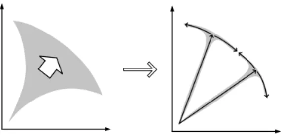
Fig. 2. Parallel speed-up framework: replacing one “▽”-tree by multiple “T”-trees.
to the weight vectors. More concretely, we manage to independently guide the
ℓth PLS process on the basis of the ℓth weight vector λℓ, hence our framework maintains ℓ archives that are updated independently in parallel. After all PLS processes terminate, we merge their respective archives (maintained locally and in parallel) and remove dominated solutions in order to obtain a Pareto set approximation. In addition, we remark from Fig. 1(b) that there can be many branches in the middle phase of the PLS trajectory tree, which makes the tree be in a shape of a triangle “▽”. However, having too many branches in the middle phase might be unnecessary and could actually be a waste of computing effort. We hence argue that reducing the number of branches in the middle phase of PLS is a key ingredient to speed-up the search. Roughly speaking, in our framework, we try to convert the “▽”-shape trajectory tree to multiple parallel “T”-shape trajectory trees as illustrated in Fig. 2. For this purpose, we propose to review the main PLS components accordingly, which is described in details in the next section.
3.4 Alternative Algorithm Components
As depicted in Algorithm 1, sequential PLS has three main problem-independent components: the selection step, the acceptance criterion and the neighborhood
exploration. In [4, 8], the design of these components was shown to be crucially
important for the anytime performance of sequential PLS. In this paper, we similarly discuss possible alternatives for these components, however our proposed alternatives are designed specifically with respect to the target parallel multi-search framework. For this reason, we also involve an additional component in our discussion: the boundary setting.
Alternatives for selection step. In this step, PLS selects a solution from the
current archive to explore its neighborhood. The basic strategy is to randomly select a solution from the archive, which we denote as ⟨RND⟩. Since each PLS process now has a weight vector λℓ, the other alternative that we consider
is to select the solution that has the highest weighted-sum function value, i.e., fws(x) =
∑m k=1λ
ℓ
kfk(x), which we denote as⟨HWF⟩.
Alternatives for acceptance criterion. The basic version of PLS accepts
any non-dominated solution to be included into the archive, and we denote this strategy as⟨⊀⟩. We propose the following alternative strategy denoted ⟨w>⊀⟩:
6 J. Shi, Q. Zhang, B. Derbel, A. Liefooghe and S. Verel
if a neighboring solution that has an even higher fws-value than the highest fws
-value from the archive is found, only such neighboring solutions are accepted, and if no such neighboring solution can be found, the acceptance criterion switches to accepting solutions that are non-dominated.
Alternatives for neighborhood exploration. In the basic version of PLS,
all neighboring solutions are evaluated. This can be seen as an extension of the
best-improving rule in single-objective local search, hence we denote this strategy
as⟨⋆⟩ [8]. The alternative could correspond to the first-improving rule in single-objective local search: if a neighboring solution that satisfies the acceptance criterion is found, the neighborhood exploration stops immediately and the current solution is marked as explored. In addition, after all solutions from the archive have been marked as explored using the first-improving rule, all solutions will be marked as unexplored and be explored again using the best-improving rule. We denote this alternative strategy as⟨1⋆⟩. Note here that, if the
⟨w>⊀⟩ acceptance criterion is used, the ⟨1⋆⟩ strategy changes to: if a neighboring
solution is accepted because it has an even higher fws-value than the archive’s
highest fws-value, the neighborhood exploration stops immediately, otherwise
the neighborhood exploration continues, and after all solutions in the archive have been marked as explored using the first-improving rule, all solutions will be marked as unexplored and be explored again using the best-improving rule.
Alternatives for boundary setting. We notice that the parallel PLS processes
are expected to approach the Pareto front from different directions in the objec-tive space when different weight vectors are used in the selection/acceptance step. We additionally manage to set boundaries between different PLS processes to avoid wasting computing resource. We denote the original unbounded alternative
as ⟨UB⟩, and the bounded alternative as ⟨B⟩. More precisely, in the bounded
alternative⟨B⟩, the boundaries are defined as the middle lines between adjacent weight vectors, as shown in Fig. 3. At the early stage of PLS, the space between the boundaries are relatively narrow, hence it is very likely that all solutions in the archive are outside the boundary. To prevent premature termination, we define the alternative⟨B⟩ as: the neighboring solutions outside the boundary will not be accepted, except when the archive is empty or all solutions in the archive are outside the boundary.
By combining the aforementioned alternatives, we can design different parallel PLS variants. For instance, a basic parallel PLS, which executes multiple basic PLS processes in parallel, is obtained by the combination⟨RND, ⊀, ⋆, UB⟩.
3.5 Related Works and Positioning
Liefooghe et al. [8] decompose the PLS procedure into several problem-independent components and investigate the performance of the PLS variants obtained using different alternative strategies. A similar methodology can be found in the work of Dubois-Lacoste et al. [4], which intends to improve the anytime performance of PLS. Our proposal differs from those works in the sense that we aim to speed up PLS in a parallel multi-search framework. We decompose
λ1 λ2 λ3 Boundary(λ1, λ2) Boundary(λ2, λ3) Boundary(λ1, λ3)
Fig. 3. Defining boundaries for 3 weight vectors.
the original problem by assigning different weight vectors to the parallel PLS processes, and previous works do not consider such an alternative in the setting of PLS components.
The concept of decomposition in our parallel framework is inspired by the widely-used MOEA/D framework [16], in which the original multiobjective problem is decomposed into a number of scalarized single-objective sub-problems and the algorithm tries to solve them in a cooperative manner. Derbel et al. [2] investigate the hybridization of single-objective local search move strategies within the MOEA/D framework. Besides, the multiobjective memetic algorithm based on decomposition (MOMAD) proposed by Ke et al. [7] is one of the state-of-the-art algorithms for MCOPs. At each iteration of MOMAD, a PLS procedure and multiple scalarized single-objective local search procedures are conducted. Liu et al. [11] propose the MOEA/D-M2M algorithm, which decomposes the original problem into a number of sub-problems by setting weight vectors in the objective space. In MOEA/D-M2M, each sub-problem corresponds to a sub-population and all sub-populations evolve in a collaborative way. MOEA/D-M2M is similar to the NSGA-II variant proposed by Branke et al. [1], in which the problem decomposition is based on cone separation.
Other works intend to enhance PLS by using a higher-level control frame-work. Lust and Teghem [13] propose the Two-Phase Pareto Local Search (2PPLS) algorithm which starts PLS from the high-quality solutions generated by heuristic methods. Lust and Jaszkiewicz [12] speed up 2PPLS on the multiobjective traveling salesman problem by using TSP-specific heuristic rules. Geiger [6] presents the Pareto Iterated Local Search (PILS) in which a variable neighborhood search framework is applied to PLS. Drugan and Thierens [3] discuss different neighborhood exploration strategies and restart strategies for PLS. At last, for the mUBQP problem, Liefooghe et al. [9, 10] conduct an experimental analysis on the characteristics of small-size instances and the performances of some metaheuristics, including PLS, on larger instances.
8 J. Shi, Q. Zhang, B. Derbel, A. Liefooghe and S. Verel 0 0.5 1 1.5 2 x 10⁴ 0 0.5 1 1.5 2 2.5 3x 10 4 f1 f2 PLS1 PLS2 PLS3 (a)⟨RND, ⊀, ⋆, UB⟩ 0 0.5 1 1.5 2 x 10⁴ 0 0.5 1 1.5 2 2.5 3x 10 4 f1 f2 PLS1 PLS2 PLS3 (b)⟨HWF, ⊀, ⋆, UB⟩ 0 0.5 1 1.5 2 x 10⁴ 0 0.5 1 1.5 2 2.5 3x 10 4 f1 f2 PLS1 PLS2 PLS3 (c)⟨HWF, w>⊀, ⋆, UB⟩ 0 0.5 1 1.5 2 x 10⁴ 0 0.5 1 1.5 2 2.5 3x 10 4 f1 f2 PLS1 PLS2 PLS3 (d)⟨HWF, w>⊀, 1⋆, UB⟩ 0 0.5 1 1.5 2 x 10⁴ 0 0.5 1 1.5 2 2.5 3x 10 4 f1 f2 PLS1 PLS2 PLS3 (e)⟨HWF, w>⊀, 1⋆, B⟩
Fig. 4. Trajectory trees of different parallel PLS variants.
4
Experimental Analysis
4.1 Pilot Experiment
To visualize the change of trajectory tree when different alternatives are used, we execute five parallel PLS variants on a {m = 2, n = 100, ρ = 0} mUBQP instance. In each execution, L = 3 PLS processes start from the same initial solution, which is randomly generated. Fig. 4 shows the trajectory trees of those five parallel PLS variants in sequence:⟨RND, ⊀, ⋆, UB⟩, ⟨HWF, ⊀, ⋆, UB⟩,
⟨HWF, w> ⊀, ⋆, UB⟩, ⟨HWF, w> ⊀, 1⋆, UB⟩ and ⟨HWF, w> ⊀, 1⋆, B⟩. In this
sequence, we alter one component of the algorithm at a time.
Fig. 4(a) shows the trajectory trees of the basic parallel PLS⟨RND, ⊀, ⋆, UB⟩, which simply runs multiple basic PLS processes in parallel. Fig. 4(b) shows the trajectory trees of ⟨HWF, ⊀, ⋆, UB⟩. By comparing Fig. 4(a) and Fig. 4(b), we can see that after changing the selection step from ⟨RND⟩ (i.e. random)
to ⟨HWF⟩ (i.e. based on the weighted-sum function), different PLS processes
are navigated to different direction in the objective space. Then, as shown in Fig. 4(c), after changing the acceptance criterion from ⟨⊀⟩ (non-dominance) to
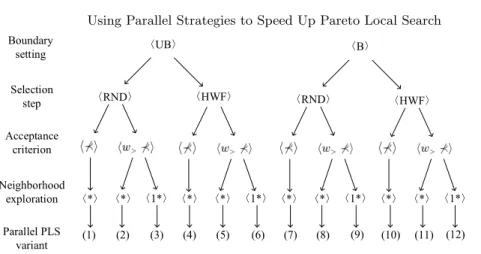
Boundary setting Selection step Neighborhood exploration Acceptance criterion 〈RND〉 〈HWF〉 〈*〉 〈B〉 〈*〉 〈1*〉 Parallel PLS variant (1) (2) (4) (5) (6) (7) (8) (9) (10) (11) (12) (3) 〈*〉 〈*〉 〈1*〉 〈*〉 〈*〉 〈1*〉 〈*〉 〈*〉 〈1*〉 〈RND〉 〈HWF〉 〈UB〉
Fig. 5. The 12 investigated parallel PLS variants.
branches in each trajectory tree decreases. From Fig. 4(d) we can see that, after changing the neighborhood exploration strategy from ⟨⋆⟩ (best-improvement)
to ⟨1⋆⟩ (first-improvement and best-improvement), the branch number in each
trajectory tree is further reduced. Actually, in Fig. 4(d) the search trajectory of each PLS process is a single-line trajectory in the middle phase of the search. In the last variant, we set boundaries between different PLS processes, and we can see from Fig. 4(e) that the overlaps between different PLS processes are reduced. Notice that Fig. 4(e) perfectly presents the parallel multi-search framework we aim to achieve, as previously sketched in Fig. 2.
4.2 Performance Comparison
In this section, we investigate 12 different Parallel PLS (PPLS) variants. The different variants’ strategies are summarized in Fig. 5. Among the variants, PPLS-1 is the basic variant ⟨RND, ⊀, ⋆, UB⟩ as illustrated in Fig. 4(a) and PPLS-12 is the ultimate variant ⟨HWF, w> ⊀, 1⋆, B⟩ as illustrated in Fig. 4(e).
We consider 9 standard mUBQP instances by setting m = 2, density = 0.8,
n ={200, 300, 500} and ρ = {0.0, 0.5, −0.5}. On each instance, 20 runs of each
PPLS variant are performed. In each run, L = 6 parallel processes start from the same randomly-generated solution and terminate naturally. The algorithms are implemented in GNU C++ with the -O2 compilation option. The computing platform is two 6-core 2.00GHz Intel Xeon E5-2620 CPUs (24 Logical Processors) under CentOS 6.4. Table 1 shows the obtained results. We use the hypervolume metric [17] to measure the quality of the Pareto set approximations obtained by each variant, and we also record the runtime of each variant. Note here that the runtime of PPLS equals to the runtime of its slowest PLS process. In Table 1 the best metric values are marked by bold font.
From Table 1, we can see that the difference of hypervolume-values between different variants is relative small, which means that all variants get approx-imately the same solution quality. In general the variants without boundaries (i.e. PPLS-1,· · ·, PPLS-6) achieve slightly higher hypervolume values than the variants with boundaries (i.e. PPLS-7,· · ·,PPLS-12). It is because, when there is no boundary, the overlaps between the PLS processes increase the chance to
10 J. Shi, Q. Zhang, B. Derbel, A. Liefooghe and S. Verel Table 1. Experimental results of the 12 PPLS variants.
PPLS-1 PPLS-2 PPLS-3 PPLS-4 PPLS-5 PPLS-6 PPLS-7 PPLS-8 PPLS-9 PPLS-10 PPLS-11 PPLS-12 n ρ Average hypervolume (×109) -0.5 7.948 7.948 7.949 7.949 7.949 7.948 7.938 7.939 7.942 7.942 7.943 7.943 200 0.0 4.008 4.008 4.008 4.009 4.009 4.008 4.000 4.006 4.006 4.005 4.005 4.000 0.5 1.296 1.295 1.299 1.300 1.300 1.300 1.294 1.295 1.297 1.297 1.295 1.296 -0.5 28.55 28.56 28.57 28.57 28.57 28.58 28.52 28.52 28.56 28.56 28.56 28.52 300 0.0 14.44 14.45 14.46 14.45 14.45 14.45 14.40 14.39 14.42 14.42 14.42 14.42 0.5 3.753 3.752 3.755 3.750 3.750 3.751 3.739 3.738 3.741 3.736 3.734 3.738 -0.5 124.47 124.46 124.50 124.50 124.49 124.48 124.24 124.23 124.35 124.4 124.41 124.39 500 0.0 62.74 62.74 62.79 62.78 62.77 62.77 62.43 62.44 62.48 62.54 62.51 62.49 0.5 15.38 15.38 15.40 15.41 15.40 15.40 15.32 15.33 15.37 15.32 15.31 15.31 n ρ Average runtime (s) -0.5 1310.41 1371.06 1194.99 547.25 546.30 516.81 219.53 356.07 48.00 22.91 21.10 19.56 200 0.0 9.91 10.98 10.87 7.21 7.04 7.27 2.50 2.98 0.43 0.22 0.20 0.20 0.5 73.52 86.51 85.54 38.59 38.17 39.23 20.31 26.08 3.18 1.69 1.75 1.59 -0.5 122.89 130.12 109.57 52.95 53.79 49.30 88.46 97.65 77.81 36.84 39.57 35.39 300 0.0 1.29 1.20 1.18 0.61 0.54 0.59 1.00 0.96 0.80 0.45 0.46 0.42 0.5 10.77 10.81 10.50 4.84 4.71 4.32 6.55 7.00 5.41 2.97 2.99 2.81 -0.5 3193.27 3350.61 2592.14 2013.39 1935.30 1574.11 363.24 554.65 210.56 147.73 171.51 151.51 500 0.0 43.89 49.51 44.88 22.53 23.01 23.13 4.07 5.65 3.36 2.32 2.36 2.21 0.5 287.82 326.62 275.87 125.07 122.76 118.43 30.49 62.49 12.50 7.93 7.62 7.59
find better solutions. On the contrary, the runtime difference between different variants is relatively large. We can see that the variants with boundaries are significantly faster than the variants without boundaries. It is because, within the bounded strategy, each PLS process only needs to search in a limited region of the objective space. Among all variants, PPLS-3 and PPLS-4, i.e.
⟨RND, w> ⊀, 1⋆, UB⟩ and ⟨HWF, ⊀, ⋆, UB⟩, get the highest hypervolume in
most cases. Compared to the basic variant PPLS-1, PPLS-3 does not show an obvious speedup, while PPLS-4 does. Indeed, on most instances PPLS-4 reaches a higher hypervolume with a much smaller runtime than PPLS-1. Among all variants, PPLS-12, i.e.⟨HWF, w>⊀, 1⋆, B⟩, is the one with the overall smallest
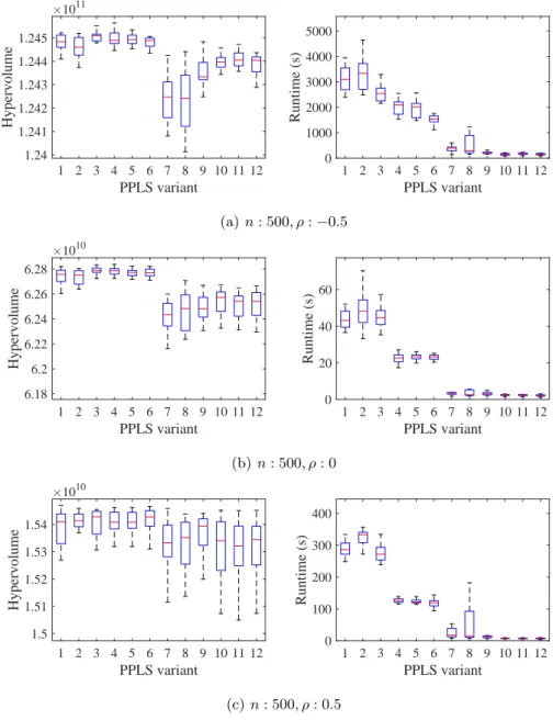
runtime. At last, Fig. 6 reports the boxplots of hypervolume and runtime of the PPLS variants on the three instances with n = 500 variables. We can see that the proposed parallel strategies can speed up the basic PLS with a relatively small loss in terms of approximation quality. In particular, while the obtained hypervolume decreases slightly when using the bounded strategy (for ρ < 0, i.e. conflicting objectives), the gap with the unbounded strategy in terms of runtime is consistently much more impressive.
5
Conclusions
In this paper, several speed-up strategies for PLS have been investigated. Compared to the existing works, our strategies are proposed in a parallel multi-search framework. In addition, we propose a diagram called trajectory tree to visualize the search process of PLS. In our experiments, we test the performance of 12 different parallel PLS variants on nine mUBQP instances with two objectives. Each variant is a unique combination of the proposed parallel strategies. The experimental results show that, compared against the basic parallel PLS variant, some variants can get a better solution quality with a shorter runtime, and some variants can significantly speed up PLS while maintaining approximately the same solution quality. In the future, we plan
1 2 3 4 5 6 7 8 9 10 11 12 PPLS variant 1.24 1.241 1.242 1.243 1.244 1.245 Hypervolume ×1011 1 2 3 4 5 6 7 8 9 10 11 12 PPLS variant 0 1000 2000 3000 4000 5000 Runtime (s) (a) n : 500, ρ :−0.5 1 2 3 4 5 6 7 8 9 10 11 12 PPLS variant 6.18 6.2 6.22 6.24 6.26 6.28 Hypervolume ×1010 1 2 3 4 5 6 7 8 9 10 11 12 PPLS variant 0 20 40 60 Runtime (s) (b) n : 500, ρ : 0 1 2 3 4 5 6 7 8 9 10 11 12 PPLS variant 1.5 1.51 1.52 1.53 1.54 Hypervolume ×1010 1 2 3 4 5 6 7 8 9 10 11 12 PPLS variant 0 100 200 300 400 Runtime (s) (c) n : 500, ρ : 0.5
Fig. 6. Experimental results on three mUBQP instances with n = 500.
to investigate the performance of the proposed approaches on multiobjective combinatorial problems with different characteristics and to investigate the scalability of the parallel PLS variants.
Acknowledgments. The work has been supported jointly by the Research Grants Council of the Hong Kong Special Administrative Region, China (RGC Project No. A-CityU101/16) and the French national research agency (ANR-16-CE23-0013-01) within the ‘bigMO’ project.
12 J. Shi, Q. Zhang, B. Derbel, A. Liefooghe and S. Verel
References
1. Branke, J., Schmeck, H., Deb, K., et al.: Parallelizing multi-objective evolutionary algorithms: Cone separation. In: Evolutionary Computation, 2004. CEC2004. Congress on. vol. 2, pp. 1952–1957. IEEE (2004)
2. Derbel, B., Liefooghe, A., Zhang, Q., Aguirre, H., Tanaka, K.: Multi-objective local search based on decomposition. In: International Conference on Parallel Problem Solving from Nature. pp. 431–441. Springer (2016)
3. Drugan, M.M., Thierens, D.: Stochastic Pareto local search: Pareto neighbourhood exploration and perturbation strategies. Journal of Heuristics 18(5), 727–766 (2012) 4. Dubois-Lacoste, J., L´opez-Ib´a˜nez, M., St¨utzle, T.: Anytime pareto local search.
European journal of operational research 243(2), 369–385 (2015)
5. Ehrgott, M.: Multicriteria optimization. Springer Science & Business Media (2006) 6. Geiger, M.J.: Decision support for multi-objective flow shop scheduling by the Pareto iterated local search methodology. Computers & industrial engineering 61(3), 805–812 (2011)
7. Ke, L., Zhang, Q., Battiti, R.: Hybridization of decomposition and local search for multiobjective optimization. IEEE transactions on cybernetics 44(10), 1808–1820 (2014)
8. Liefooghe, A., Humeau, J., Mesmoudi, S., Jourdan, L., Talbi, E.G.: On dominance-based multiobjective local search: design, implementation and experimental analysis on scheduling and traveling salesman problems. Journal of Heuristics 18(2), 317–352 (2012)
9. Liefooghe, A., Verel, S., Hao, J.K.: A hybrid metaheuristic for multiobjective unconstrained binary quadratic programming. Applied Soft Computing 16, 10–19 (2014)
10. Liefooghe, A., Verel, S., Paquete, L., Hao, J.K.: Experiments on local search for bi-objective unconstrained binary quadratic programming. In: EMO-2015 8th International Conference on Evolutionary Multi-Criterion Optimization. vol. 9018, pp. 171–186 (2015)
11. Liu, H.L., Gu, F., Zhang, Q.: Decomposition of a multiobjective optimization problem into a number of simple multiobjective subproblems. IEEE Transactions on Evolutionary Computation 18(3), 450–455 (2014)
12. Lust, T., Jaszkiewicz, A.: Speed-up techniques for solving large-scale biobjective TSP. Computers & Operations Research 37(3), 521–533 (2010)
13. Lust, T., Teghem, J.: Two-phase Pareto local search for the biobjective traveling salesman problem. Journal of Heuristics 16(3), 475–510 (2010)
14. Paquete, L., Chiarandini, M., St¨utzle, T.: Pareto local optimum sets in the biobjective traveling salesman problem: An experimental study. In: Metaheuristics for Multiobjective Optimisation, pp. 177–199. Springer (2004)
15. Paquete, L., Schiavinotto, T., St¨utzle, T.: On local optima in multiobjective combinatorial optimization problems. Annals of Operations Research 156(1), 83– 97 (2007)
16. Zhang, Q., Li, H.: MOEA/D: A multiobjective evolutionary algorithm based on decomposition. Evolutionary Computation, IEEE Transactions on 11(6), 712–731 (2007)
17. Zitzler, E., Thiele, L., Laumanns, M., Fonseca, C.M., Da Fonseca, V.G.: Performance assessment of multiobjective optimizers: An analysis and review. IEEE Transactions on evolutionary computation 7(2), 117–132 (2003)