Characterizing non-coding hits in genome-wide association studies using epigenetic data

ARCHvs

JUL 0 8 2013

LIBRARIES

Characterizing non-coding hits in genome-wide

association studies using epigenetic data

by

Abhishek Kulshreshtha Sarkar

B.S. Computer Science, University of North Carolina at Chapel Hill, 2011

Submitted to the Department of Electrical Engineering and Computer Science in partial fulfillment of the requirements for the degree of

Master of Science in Electrical Engineering and Computer Science at the

Massachusetts Institute of Technology June 2013

@ Massachusetts Institute of Technology 2013. All rights reserved.

Author

Department of Electrical Engineering and Computer Science May 22, 2013

Certified by

Manolis Kellis Associate Professor of Electrical Engineering and Computer Science Thesis Supervisor n

Accepted by

Li4 A. Kolodziejski Chair, Department Committee on Graduate Students

Characterizing non-coding hits in genome-wide association studies

using epigenetic data

by

Abhishek Kulshreshtha Sarkar

Submitted to the Department of Electrical Engineering and Computer Science on May 22, 2013 in partial fulfillment of the requirements for the degree of

Master of Science in Electrical Engineering and Computer Science

Abstract

Understanding the molecular basis of human disease is one of the greatest challenges of our time, and recent explosion in genetic and genomic datasets are finally putting it within reach. In the last ten years, genome-wide association studies have identified thousands of genetic variants associated with disease. However, the majority of these variants fall outside genes making interpreting their role in disease difficult. In parallel, the ENCODE and Roadmap Epigenomics consortia have produced high resolution annotations of the genome which identify large portions with potential regulatory function. We develop methods to interpret genome-wide association studies using these annotations to generate hypotheses about how associated variants contribute to disease mechanism. In particu-lar, we go beyond the usual stringent p-value threshold to investigate variants with small individual effect sizes which current methods do not have power to detect. Evaluating our methods on the Wellcome Trust Case Control Consortium 7 Disease studies, we find associated variants are enriched in a variety of functional categories even after control-ling for various biases. We also find an unprecedented number of variants contribute to this enrichment, supporting our hypothesis that the architecture of these diseases involves combinatorial interaction of many variants with small individual effect sizes.

Thesis supervisor: Manolis Kellis

Contents

1 Introduction 4

2 Background information 6

2.1 Inheritance . . . . 6

2.2 Genes and regulation . . . . 6

2.3 Linkage analysis . . . . 8

2.4 The common disease, common variants hypothesis . . . . 9

2.5 Genome-wide association studies . . . . 10

2.6 The missing heritability problem . . . . 11

2.7 Epigenetics . . . .. . . . . 12

3 Genome-wide enrichments of functional elements 14 3.1 Methods ... ... 14 3.1.1 Functional annotations . . . . 14 3.1.2 GWAS Data . . . . 14 3.1.3 Statistical analysis . . . . 15 3.1.4 Related w ork . . . . 16 3.2 R esults . . . . 18

3.2.2 Implicated enhancers appear genome-wide . . . . 21

3.2.3 Implicated enhancers are independent of known associated loci . . . 22

3.2.4 Implicated enhancers are cell type-specific . . . . 24

3.2.5 Open chromatin is enriched for disease-associated variants . . . . . 26

4 Pathway analysis 29 4.1 M ethods . . . . 29

4.1.1 Region-based tests for enrichment of pathways . . . . 29

4.1.2 SNP-based exact rank sum test for enrichment of pathways . . . . . 30

4.1.3 Related w ork . . . . 30

4.2 R esults . . . . 31

4.2.1 Enrichment of T1D-associated variants . . . . 31

4.2.2 Enrichment of enhancer regions . . . . 31

4.2.3 Enrichment of T1D-associated regulatory variants . . . . 31

4.2.4 Enrichment of enhancer clusters . . . . 33 4.2.5 Enrichment of T1D-associated cell type-specific regulatory variants 36

Acknowledgments

This thesis would not have been possible without the help and support of friends, col-leagues, and family:

Aaron Sidford, whose Not So Great Ideas in Theoretical Computer Science were a welcome diversion.

The MIT Computational Biology Group for their feedback and suggestions.

Wouter Meuleman for his assistance with enhancer clustering and pathway analysis. Luke Ward for his biological insight and assistance with developing and refining the meth-ods.

Manolis Kellis for his enthusiasm and mentorship.

Chapter 1

Introduction

Understanding the molecular basis of human disease is one of the greatest challenges of our time, and recent explosion in genetic and genomic datasets are finally putting it within reach. In the last ten years, genome-wide association studies (GWAS) have identified thou-sands of genetic variants associated with disease. However, the majority of these variants fall outside genes making interpreting their role in disease difficult. The first step in go-ing from GWAS to explaingo-ing disease is to generate high quality hypotheses about which disease-associated variants are causal and how they contribute to the disease mechanism. The difficulty up to this point has been a lack of understanding of the non-coding genome. The ENCODE and Roadmap Epigenomics consortia have now produced high res-olution annotations of the genome which identify large portions with potential regula-tory function. In particular, ChromHMM learns combinations of chromatin modifications which are enriched in regions with particular function. Annotating the genome with the most likely hidden state at each point gives an unparalleled resource for interpreting non-coding variants. Indeed, current work has begun to show top GWAS hits fall dispropor-tionately in regulatory regions. It is now possible link these regions to their target genes and determine the proteins they recruit to regulate their targets and where they bind. With these rich annotations in hand current work can more confidently identify causal variants and generate highly specific mechanistic hypotheses about their contribution to disease pathology.

However, it is also known that GWAS lacks sufficient power to detect all but the most deleterious variants due to small sample sizes and human population genetic biases. The next key challenge in understanding complex polygenic disease is identifying causal vari-ants in the long tail of the p-value distribution.

The goals of this thesis are three-fold. The first is to develop methods to use reg-ulatory annotations and investigate the whole spectrum of GWAS p-values rather than only the top hits which pass the usual p-value threshold. We hypothesize complex traits arise from large numbers of variants with small individual effect sizes. These variants es-cape detection because typical p-value cutoffs are too stringent and samples sizes are not large enough. However, the ranking of SNPs by association to trait still gives some par-tial information which should contribute to genome-wide trends of over-representation in functional regions of the genome.

(T1D) and identify variants which are enriched. In particular, we should identify variants beyond the usual stringent p-value threshold which have smaller effect sizes. We also aim to identify relevant regulatory regions and the cell types which they are active in.

The third goal is to interpret the role of identified variants in disease. We should be able to make mechanistic hypotheses about how the variants we identify contribute to the disease. In particular, we look for gene pathways which are enriched for disease-associated variants.

The contributions of this thesis are two-fold. First, the methods should be generally applicable to complex polygenic traits. They should give some insight which will direct further investigation on the genetic architecture of these traits. Second, our results on T1D should reveal new insights about the disease biology which could be used to develop predictive models, diagnostics, and potential treatments.

Chapter 2

Background information

2.1

Inheritance

Near the turn of the 2 0 th century, researchers rediscovered the work of Gregor Mendel,

whose experiments on peas elucidated the particulate nature of inheritance. This work became the basis of the nascent field of genetics. But it took another half century for Watson and Crick to discover the molecular basis of inheritance, the double helical

poly-mer deoxyribonucleic acid (DNA) [46]. DNA is a polypoly-mer of nucleotides (or bases): adenine,

thymine, guanine, and cytosine (represented "A", "T", "G", "C"). The four nucleotides ap-pear in two complementary pairs due to hydrogen bonding: adenine with thymine and guanine with cytosine. The primary sequence is paired with its reverse complement in the double helix structure. DNA is further structured into discrete molecules called

chromo-somes.

By the 1 9 th century, scientists had already observed the role of DNA in asexual

repro-duction. In the process of mitosis, enzymes replicate the DNA exactly and divide the two copies among the two daughter cells. In the late 1800s, researchers observed the process

of meiosis which is required for sexual reproduction. Diploid organisms (such as humans)

have two homologous copies of each chromosome. However, they produce haploid cells (which only have one copy) called gametes which combine in the process of

fertilization

produce a new diploid organism. Meiosis is initially identical to mitosis. However, after two diploid cells are produced each immediately divides into two haploid cells.

2.2

Genes and regulation

DNA is often called the "genetic code". In particular, regions of the sequence called genes

are transcribed into ribonucleic acid (RNA). RNA is a single-stranded polymer similar to

DNA, but substituting the nucleotide uracil for thymine. While DNA is confined to the nucleus of the cell, RNA can move out of the nucleus. Outside of the nucleus, cell

machin-ery translates RNA into proteins. Codons (words of length 3) in the DNA/RNA sequence

correspond to amino acids, the building blocks of proteins.

There are two key observations to make about this code. First, we now know less than 2% of the genome codes for proteins (although significantly more is transcribed into

ONA

methylation

Chromatin

modifications DNase Ihypersensitive

sites Functional genomic elements Histone Nucleosome Transcription-factor binding sites

Transcr ption Transcription

DNA factor mnachinery

Long-range Promoter Protein-coding

regulatory architecture and non-coding

elements transcripts

Chromosome~

Figure 2.1: Illustration of regulatory regions and mechanisms [7]. The primary sequence

(bottom) contains transcribed regions such as genes whose expression is regulated at

short-range by promoters and long-short-range by enhancers. Transcription factors bind to the

se-quence and can form large complexes (center). The DNA molecule itself undergoes

chemi-cal modifications (top left) and changes conformation (top right) to change the accessibility

of the primary sequence.

RNA). Second, every cell in complex organisms such as humans contains the same primary

sequence of DNA. These observations raise the question of why we observe a huge variety

of human cell types with diverse physical traits and functions.

We now know there is more encoded in the DNA sequence than just proteins.

An-other portion of the genome has regulatory function, modulating the expression (level of

transcription) of genes. Figure 2.1 shows a variety of regulatory regions. Promoters are

directly upstream of genes and are responsible for recruiting the transcription

factors (TFs)

which transcribe DNA. The structure of TFs is such that they bind to specific DNA

se-quence motifs (short words of length 8-16). TFs can also recruit other TFs to form larger

complexes which are necessary to start transcription of some genes. More distant regions

called enhancers also recruit TFs through motifs. TFs bound to enhancers can interact with

promoters and genes because the DNA molecule can fold to bring these regions close

to-gether.

Indeed, there is a complex network of interactions between genes and regulators. The output of one gene may be a regulator which targets another, related gene. Larger gene

pathways are sets of related or linked genes which together contribute to a coherent cell

function.

2.3

Linkage analysis

In 1911, Morgan observed crossover recombination in D. melanogaster (fruit fly) meiosis. In one phase of meiosis, the chromosomes are arranged in the middle of the cell. During this phase, homologous chromosomes can cross over each other and exchange contigu-ous subsequences of DNA. Morgan realized the frequency of crossover recombination be-tween two points on a chromosome was proportional to the distance bebe-tween them. Thus, Mendel's hypothesis genes were inherited independently was wrong. This phenomenon, where genes are inherited together, is called linkage disequilibrium (LD). In 1913, Morgan and Sturtevant used this observation to develop the first linkage map and localized genes driving fly phenotypes (traits). Such a map gives not only the order of genes on the chromo-some but also their relative distance to each other. A distance of 1 centimorgan corresponds to a .01 probability of recombination between two points on the chromosome.

Figure 2.2 shows linkage disequilibrium patterns for a region of chromosome 5. Pair-wise LD is visualized as a lower-triangular matrix, where each point corresponds to a pair of SNPs and the amount of red represents the strength of correlation. Strong LD patterns are outlined in black and demarcate blocks of nearby SNPs which are only rarely separated by recombination.

Linkage analysis is the problem of finding DNA variation which cosegregates (is

inher-ited together) with a trait of interest. If the DNA variant is inherinher-ited along with the trait, it must lie close or be "linked" to the gene driving the trait because recombination was not observed to separate the two. In the late 1970s, methods for cloning [20] and sequenc-ing [32] DNA made it possible to tie linkage maps to the underlysequenc-ing sequence and clone linked genes. However, building genome-wide linkage maps in human was infeasible because few genetic markers (known positions on a chromosome) were known.

In 1980, Botstein proposed using restriction

fragment length polymorphisms to build

link-age maps [3]. Restriction enzymes are proteins which cut DNA at specific sequence motifs. Applying a restriction enzyme to the whole genome gives a particular distribution of frag-ment lengths. Variations in the sequence can either remove or introduce such motif

in-stances, changing this distribution.

With genome-wide linkage maps in hand, positional cloning became the paradigm for uncovering the molecular basis of traits. Such experiments identified linked regions, se-quenced those regions in cases (subjects who have the trait) and controls (who do not), and thereby identified the causal genes. The first success of this method was the discovery of the mutation driving Huntington's disease [12].

Given the subsequent success of this method in uncovering the basis of Mendelian traits arising from a single mutation/gene, geneticists hoped to be able to explain traits like common diseases. They found Mendelian subtypes of some common diseases, but the identified causal genes explained very few of the cases in the population. Indications

CHI1N1

IIU11hUELijIP

Figure 2.2: Patterns of LD in the genomic region 5q31 [1]. Pairwise correlation is displayed

on the lower triangular matrix, where red is r

1. Strong correlation (outlined in black)

demarcates blocks of nearby SNPs; however, we also observe long range correlations due

to limited recombination.

suggested these traits arise from many genes. Indeed, in 1910 East proposed common

traits are polygenic [6] and in 1919 Fisher proposed a model of how many discrete variants

could lead to continuous traits [11].

2.4 The common disease, common variants hypothesis

Model organism geneticists working on yeast and fly have the ability to construct large

crosses and therefore trace inheritance of complex polygenic traits and genetic variants

through large pedigrees. Human geneticists did not have this luxury; instead they turned

to insights from population and evolutionary genetics.

First, the human population has grown exponentially only recently on an

evolution-ary time scale. Evolutionevolution-ary theory thus predicts limited genetic variation in the

popu-lation. Indeed, single nucleotide polymorphisms (SNPs) occur on average only once every

thousand base pairs. These naturally occurring DNA variants are single bases which take

multiple alleles (possibilities) in the population. Most of these variants only take one of two

alleles, called major and minor based on their relative frequency in the population.

More-over, the majority of these variants are common (i.e. the minor allele appears in more than

5% of the population).

Second, many Mendelian diseases arise from rare variants. These variants have large

effects on reproductive success, so evolutionary theory predicts selection will drive their

frequency to zero. On the other hand, common disease has smaller effect on reproductive

fitness and so variants causing such traits could arise to higher frequency in the

popula-tion. This outcome is facilitated by the recent growth in the human populapopula-tion. Moreover,

rs6679677 AA AC CC Controls 84 1902 8602 T1D Cases 62 541 1359

Table 2.1: Genotype counts for an example GWAS tag SNP. This SNP tags a locus known to be associated with Type 1 Diabetes and shows a different distribution of counts in cases than in controls. The p-value for a 2 degree of freedom chi-square test on this contingency

table is p = 6.5 x 10-39

in some cases heterozygotes (having one risk allele) for disease-causing variants have an advantage over their homozygote counterparts (having no risk alleles). For example, sickle-cell anemia heterozygotes show increased resistance to malaria. Thus, human geneticists proposed common diseases arise from common variants.

2.5

Genome-wide association studies

To actually find common variants causing common disease in genome-wide association

stud-ies (GWASs), geneticists had to achieve three goals. First, they had to build comprehensive

catalogs of SNPs in the human population. The HapMap consortium has sequenced over one thousand individuals and has published a catalog of over 2 million common SNPs [39, 40, 41]. More recently, the Thousand Genomes Project consortium has sequenced a comparable number of individuals using the latest sequencing technology and published a catalog of 38 million SNPs including rare variants [37].

Second, they had to develop methods to quickly and cheaply genotype these variants in large panels of individuals. Here, they were aided LD. As shown in Figure 2.2, SNPs occur in large blocks in which no recombination has occurred. Thus the genotypes of common SNPs can be inferred from just the genotypes of carefully chosen tag SNPs.

To actually genotype these tag SNPs, they developed DNA microarrays [44]. The array itself is a large library of DNA fragments called probes with one end anchored to a

chip. The experiment amplifies and fragments the sample DNA, attaches fluorescent tags

to the fragments, and hybridizes the fragments to the probes. They recover the original genotypes by observing the light intensity at each probe.

Third, they had to develop the statistics to analyze the patterns of genotypes in the cohorts of cases and controls. At a basic level, GWAS performs one hypothesis test per

locus (a region of the genome represented by the tag SNP, but also containing all of the

common SNPs in LD with the tag). There are two frequently tested null hypotheses: the distribution of allele counts is independent between cases and controls, or the distribution of genotype counts is independent. Table 2.1 shows an example set up for testing the null hypothesis the distributions of genotypes between controls and Type 1 Diabetes cases at a

particular tag SNP are independent. One issue is conducting millions of such tests inflates

the false positive rate and requires stringent correction. The usual method is Bonferroni correction (dividing the desired false positive rate a by the total number of tests) which is known to be over-conservative.

A more difficult problem is accounting for sources of genetic variation which are

known to not be related to phenotype. One obvious confounder is familial relation be-tween subjects, which violates the independence assumption underlying the statistical testing. But another consequence of the recent human population expansion is genome-wide allele frequency differences associated with ethnicity (i.e. human subpopulations). One possible way to account for these biases is to simply choose subjects such that they are unrelated and come from the same ethnic background. Statistically correcting for this bias in cohorts of mixed ethnicities requires more sophisticated methods such as genomic control, principal components analysis, or learning mixed models. Technical artifacts of the genotyping technology are another unavoidable confounder, but the error rates of the technologies are steadily decreasing.

2.6 The missing heritability problem

To date, thousands of loci have been associated with hundreds of traits [15]. Many of these loci are independent, further supporting the polygenic basis of complex traits. However, the vast majority do not lie in or near genes, making interpreting their function difficult. Moreover, those variants which have been independently reproduced in follow-up stud-ies still explain only a fraction of the heritability of these traits [23, 24, 8]. Heritability is the proportion of phenotypic variation explained by genetic variation. Obviously, other factors beyond genetics contribute to the instances of common disease in the population. However, the fraction of heritability of common disease explained by known variants does not match the fraction of heritability attributable to genetics based on tracing these diseases through pedigrees.

There are multiple competing hypotheses about where this missing heritability can be found. First, one previously inaccessible source is rare, private mutations. These are not captured by DNA microarrays, but can be efficiently genotyped by current sequencing technology. Second, another potential source is DNA structural variants, such as inser-tions, deleinser-tions, inversions, repeats, and other rearrangements of the sequence. Again, it is only with the latest technology that genome-wide detection of these variants has become feasible.

Third, common variants could indeed explain the heritability of complex traits but have too low individual effect sizes to be detected by current methods. One concern is that the statistical power of genome-wide association studies is limited by the size of the case and control cohorts. Some progress has been made on this front by pooling data across studies and performing meta-analysis. Fourth, variants and genes interact with each other non-additively to contribute to complex traits. Many computational models have been proposed to learn such interactions from genotype data; however, they have to bound the degree of interaction terms to make analysis tractable and still leave much heritability unexplained.

Recent work on the genetic basis of human height lends weight to these last two hy-potheses [30, 19]. Height is estimated to be 80% heritable. Although some rare variants have been found which explain extreme values of the phenotype, they explain only a mi-nority of cases. Roughly 50 SNPs have been associated with height in GWASs; however,

they explain only 5% of the heritability. However, by considering the entire GWAS panel of SNPs we can explain roughly 45% of the heritability of height.

2.7

Epigenetics

Parallel to these developments in understanding the role of DNA as genetic code and lo-calizing causal variants for traits, we have also learned there is more to the molecule than simply the primary sequence. In particular, there are heritable molecular traits which are not explained by the primary sequence. One example is DNA methylation, in which indi-vidual cytosine nucleotides are modified with an additional methyl (CH3) group.

Methy-lation is now known to serve as a silencer of DNA function, and current work seeks to understand both how the primary sequence and disease traits can change methylation across the genome.

Epigenetics also refers more generally to molecular factors other than the primary DNA

sequence which can affect traits. As described previously, the DNA molecule is divided into chromosomes. The structure of chromosomes involves several nested levels of struc-ture as shown in Figure 2.1. At the lowest level, the DNA double helix is wrapped around protein complexes called nucleosomes, each constructed of four proteins called histones. His-tones themselves are accepting of modifications such as methylation and acetylation. Hun-dreds of these modifications, called chromatin marks, have been discovered experimentally, leading to the hypothesis they also encode part of the function of DNA. For example, H3K4Me3 (trimethylation of the 4th amino acid in histone 3) is associated with nearby promoter activity.

Chromatin modifications are measured using chromatin immunoprecipitation followed by high-throughput sequencing (ChIP-Seq). The experiment uses restriction enzymes frag-ment the DNA. Specifically selected antibodies are used to select fragfrag-ments bound to pro-teins of interest (such as histones with a particular modification). The fragments are then sequenced and aligned to a reference genome to localize their position.

We do not know a priori the function associated with individual marks, nor whether they act independently. Ernst instead used an unsupervised approach to learn "chromatin states", hidden states of a multivariate HMM [9]. The emission alphabet of the HMM is combinations of chromatin marks; the hidden states correspond to biological functions which change the probability of observing particular combinations. By learning the HMM over the whole genome, we get a high resolution map of regions which are likely pro-moters, enhancers, repressors, transcribed elements, etc. For example, Figure 2.3 shows the annotation of the WLS gene across nine human cell types. This gene is important in eukaryotic development in aligning one axis of symmetry. The gene is is predicted to be transcribed (green) in five of the cell types. In those cell types, we find an active enhancer (yellow). However, in the others the gene is quiescent (not expressed; gray). We find the promoter is poised (purple): although transcription factors are bound to it the gene is not being transcribed. Poised regulators are needed for rapid, time-dependent regulation of

genes which is necessary in the development of embryos.

Beyond wrapping around histones, the DNA molecule is further condensed into a dense structure called chromatin. It is important to note the primary sequence is

inacces-Scale 10 kb| | hg19

chr1 68,620,00d 68,625,004 68,630,004 68,635,00d 68,640,004 68,645,00d 68,650,00d 68,655,00d

UCSC Genes (RefSeq, UniProt, CCDS, Rfam, tRNAs & Comparative Genomics)

UCSC Genes --

---Chromatin State Segmentation by HMM from ENCODE/Broad GM12878 ChromHMMIU H1-hESC ChromHMM K562 ChromHMM HepG2 ChromHMM HUVEC ChromHMM HMEC ChromHMM, HSMM ChromHMMIU NHEK ChromHMM-NHLF ChromHMM1

Figure 2.3: Chromatin state annotations of the region containing the WLS gene across nine human cell types. The gene is expressed (green) in five of the cell types. In these cell types we can identify a nearby strong enhancer (yellow). The promoter is poised (purple) but

the gene is inactive (gray) in the other cell types.

sible in regions which are so condensed, as shown in Figure 2.1. Thus, whether or not chromatin is open is another indication of regulatory function. There are several exper-imental approaches to identify open chromatin, such as DNAseI hypersensitivity (DHS) and Digital Genomic Footprints (DGF) [14]. In essence, these methods all use restriction enzymes to cut DNA where it is accessible, sequences the fragments, and aligns them to a reference genome to localize their position.

Epigenetic modifications are an invaluable resource in interpreting the role of the non-coding part of the genome. Towards this end, the ENCODE Consortium has produced chromatin state maps of nine human cell lines and DHS/DGF in ninety [38]. The NIH Roadmap Epigenomics Consortium has produced complete epigenomes of 85 primary human cell types including methylation, gene expression (by extracting and sequencing RNA), and chromatin state maps [2].

Chapter 3

Genome-wide enrichments of

functional elements

We have introduced the paradigm of genome-wide association studies and described how potentially many undiscovered loci could escape detection. We also introduced regulatory elements which control gene expression and are known to play some role in disease. Now, we describe our contributions in combining these data to identify large numbers of small effect size, potentially causal variants.

3.1

Methods

3.1.1 Functional annotations

We use ChromHMM annotations for nine ENCODE cell lines downloaded from the UCSC Genome Browser. We also use currently unpublished ChromHMM annotations for 85 Roadmap Epigenomics primary cell types (intersecting replicates) from the Analysis Work-ing Group. We use DHS and DGF annotations for 90 ENCODE cell lines downloaded from the UCSC Genome Browser. We use long poly-A+ RNA-Seq contigs in 9 ENCODE cell lines to produce annotations of discretized expression downloaded from the European Bioinformatics Institute (accessed through the UCSC ENCODE portal).

3.1.2

GWAS Data

We revisit the Wellcome Trust Case Control Consortium 7 Diseases studies [42]. These studies investigate common diseases: bipolar disorder, coronary artery disease, Crohn's disease, hypertension, rheumatoid arthritis, Type 1 Diabetes, and Type 2 Diabetes. Each study involves a cohort of 2,000 cases and a shared set of 3,004 controls. All subjects were of British descent and were chosen to be unrelated. The controls were taken from two sources: the UK National Blood Service and the 1958 British Birth Cohort.

The cohorts were genotyped on the Affymetrix 500K SNP array, capturing just under 500,000 common SNPs. They were then imputed to the HapMap 3 common variants, yield-ing genotypes for 2.6 million common SNPs. P-values were computed usyield-ing a 1 degree of freedom chi-square test for independence of allele counts between cases and controls.

We focus on the GWAS for Type 1 Diabetes (T1D). This disease is a classical example of a common, polygenic disease [13]. The disease pathology involves autoimmune de-struction of beta cells in the pancreas which produce insulin. Those with the disease must inject insulin into their bloodstream to maintain healthy levels of blood sugars.

There is a Mendelian subtype of T1D which is attributable to a single rare mutation; however, this subtype explains fewer than 1% of cases in the population. Evidence sup-ports the hypothesis hundreds of moderate-effect variants explain the disease making it an ideal disease to study. Moreover, we have regulatory annotations for a large variety of immune cells with various surface markers, giving us the opportunity to find regulators in disease-relevant cell types. These regulators are more likely to have a role in the disease, especially if they are specific to immune cells.

3.1.3 Statistical analysis

Our methods are motivated by two observations. First, the majority (roughly 80%) of trait-associated variants which have been found to date fall outside of genes. One obvious ex-planation is these variants fall in regulatory regions and contribute to disease mechanism by disrupting gene regulation. Second, evidence suggests disease-associated variants have moderate effect sizes which cannot be captured by current GWASs. They do not have large

enough sample sizes to have sufficient power to detect these variants.

In essence, we want to extend the notion of enrichment of top loci to the whole genome. Specifically, we ask whether or not variants falling in regulatory regions are skewed to have lower p-value than variants falling outside regulatory regions. To answer this question we develop a visualization called an RR plot 1. We rank the SNPs in order of increasing GWAS p-value and first compute the total number of SNPs falling in regulatory regions ("hits"). Let T be this total number. As we traverse the list, we keep a running count of how many hits we have observed and how many we would have expected as-suming hits were uniformly distributed over the list. Suppose we have seen M of N total SNPs. Then the expected count is equal to:

MT

E- N

N

Suppose in the M SNPs there were 0 SNPs observed to fall in regulatory regions. We define the normalized cumulative deviation as:

D =0-E

T

We plot this quantity every 1000 SNPs down the list to obtain the RR plot. For exam-ple, Figure 3.1 shows an RR plot for enhancers in CD4+ CD25~ IL17+ PMA/Ionomcyin-stimulated Th17 primary cells in blue and an RR plot for a permuted control set of en-hancers in red.

We make several key observations about these plots. First, the deviation is defined in such a way that the plot starts and ends at zero deviation. Second, if p-values in regula-tory regions are skewed to have lower p-values than those outside the RR plot will show

enh 0 * 0.015-CDo CL C) 0.010-E 16K overlaps n top 30K SNPs 0 78K total overiaps .2 [.005- CL Ca 0.005-0 500000 1000000 1500000 2000000 2500000

SNPs ranked by increasing p-value

Figure 3.1: Example RR plot. After seeing 30K SNPs we have encountered 1.6K overlaps

with Th1

_{enhancers where only 900 were expected (based on the total count). When we}

plot this deviation over the whole ranked list, Th17 enhancers (blue) are clearly enriched

compared to the randomized control regions (red).

larger deviation early in the ranked list. Third, the plots not only allow us to ask whether

functional regions are enriched for disease-associated variants but also how far down the

ranked list we have to go before we stop observing this enrichment. In particular, we focus

on the first part of the curve because although we hypothesize large numbers of variants

could contribute to disease we do not believe variants which are not even significant

be-fore multiple testing correction are relevant. Therebe-fore, we focus on the first 150,000 SNPs,

beyond which p-values stop being significant at the a = .05 level.

3.1.4

Related work

There are several methods published to interpret top GWAS loci using regulatory

anno-tations. Ernst revisited published associations for diseases and showed in some cases

they overlap more than expected with enhancer regions [10]. Moreover, the implicated

enhancers and the genes they target are specifically active only in disease-relevant cell

types. For example, reported associations for systemic lupus erythematosis, an

autoim-mune disease, fall in GM12878 lymphoblastoid-specific enhancers (an imautoim-mune cell type).

One of these associations tags a mutation which disrupts an Ets-1 sequence motif, which

disrupts the GM12878-specific activating transcription factor Ets-1. This SNP is therefore

hypothesized to disrupt activation of the targeted HLA-DRB1 gene, which is important for

recognition of cell surface markers and differentiating one's own cells from invaders.

Trynka used a similar approach to interpret top SNPs and strongly correlated

vari-ants in LD in four phenotypes [43]. However, rather than calling chromatin states their

approach examined chromatin marks individually. The method computes a cell type-specificity score by based on the distance to the nearest ChIP-Seq peak in each cell type. To assess significance, the score is computed for LD block size-matched control sets.

Maurano used DHS and DGF to localize GWAS hits [25]. They first used cell type-activity profiles to link DHS regions with their target genes. They next identified variants falling in TF binding sites and showed they were over-represented in binding sites for genes relevant to disease traits. They also proposed hypergeometric tests at increasing p-value thresholds as a method to identify disease-relevant cell types. We do not take this approach because it introduces another multiple testing problem.

The question of whether p-values falling in a set of regions are skewed to be lower than those falling outside the set is a well-studied problem. In particular, this problem formulation is known as the competitive null hypothesis in gene set enrichment analysis. Gene set enrichment analysis is the problem of prioritizing sets of genes (usually related by function) for further dissection. Typically, each gene is scored based on the p-value of nearby SNPs either in terms of genomic position or correlation due to LD. The competitive null hypothesis states the scores of genes in the gene set are the same as the scores of genes outside the set. Our method differs from this approach by not assigning scores to regions but rather computing statistics on the p-values of individual SNPs directly.

One obvious approach to answer this question in our setting is treating the two sets of p-values as samples and using established statistical tests. The Mann-Whitney U test is a nonparametric test of the null hypothesis the two samples are the same against the al-ternative hypothesis one sample is greater than the other. U is defined as the sum for each observation in the first sample of the number of observations in the second sample which have lower rank. This quantity has a closed-form in terms of the sums of ranks of the ob-servations in each sample. It is also approximately normally distributed. However, under this formulation the test is equivalent to one which asks whether difference of the medians of the two samples is nonzero [34]. This quantity does not capture the full distribution of the p-values, making it inappropriate for answering the question we are interested in.

The Kolmogorov-Smirnov two-sample D test is a nonparametric test of the null hy-pothesis the two samples come from the same probability distribution against the alter-native hypothesis they do not. D is defined as a function of the empirical cumulative distribution functions of the two samples. Critical values of D (needed to compute p-values) are tabulated because the statistic does not have a closed-form distribution. This test more directly answers the question of whether the p-values in the first sample (falling in regulatory regions) are skewed to be different from those in the second sample (outside). However, these two tests make independence assumptions which does not hold. First, they assume individual observations are independent. However, the two samples are p-values of SNPs and we know the genotypes of nearby SNPs are highly correlated due to LD. Therefore, the patterns of genotypes across cases and controls and therefore the p-values of nearby SNPs are also highly correlated.

Second, the they assume the two samples are independent. The patterns of genotypes in regulatory variants across cases and controls will be different from the patterns of other variants due to differential natural selection. Variants outside regulatory regions are less likely to have a role in reproductive fitness and therefore selection is less likely to apply pressure to maintain a particular genotype at those variants. On the other hand, variants

in regulatory regions are more likely to have a role and therefore selection will reduce the variability. Thus, the two samples are not independent because we gain some information about the p-values by conditioning on whether or not the SNP they correspond to falls in a regulatory region.

Statistical pitfalls aside, this approach produces easily interpreted results in identify-ing which cell types and annotations are relevant. However, the resultidentify-ing p-values do not give any indication of how many SNPs are contributing to the observed enrichment.

A second approach is to ask whether variants falling in regulatory regions are over-represented at the head of the ranked list. One obvious way to test this approach is to compute Fisher's exact p-values at a variety of cutoffs; however, this method requires further multiple testing correction.

Our approach of keeping a running deviation is used by a number of gene set en-richment methods which we draw inspiration from. In particular, the GSEA algorithm defines an enrichment score as the maximum value achieved by a walk down the ranked list where each overlap counts as +1 and each non-overlap counts as -1 [36]. However, GSEA makes the assumption few genes are involved in the trait and exponentially reduces the weight of overlaps in the running sum further down the ranked list. We do not bias our method in this manner in order to compute a new empirical cutoff beyond which we stop seeing enrichment.

3.2

Results

3.2.1

Enhancer regions are enriched for disease-associated variants

We first ask which classes of functional regions are enriched for T1D-associated variants. We compute RR plots for a variety of annotations in the GM12878 lymphoblastoid cell line:

" Promoter chromatin states " Enhancer chromatin states " Transcribed chromatin states e Repressed chromatin states e Other chromatin states

" Expressed regions (intersection of poly-A+ RNA-Seq contigs with transcribed chro-matin states)

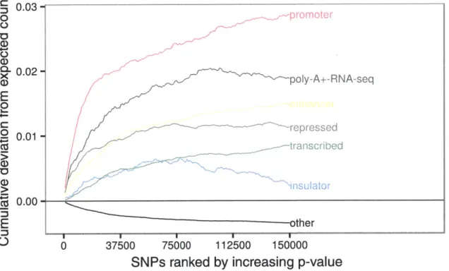
Figure 3.2 shows promoters, enhancers, transcribed regions, and expressed regions are all enriched for T1D-associated variants. We expect transcribed and expressed regions to be enriched because mutations in these regions are more likely to be non-synonymous (changing an amino acid) and therefore deleterious. We also expect promoters to be en-riched because mutations in these regions are more likely to disrupt binding sites which are necessary for the transcription of proteins, directly affecting gene expression. More-over, variants in promoters are more likely to be in LD with variants falling in the gene

40 -CS 0.03 -03 promoter CD) -L 0 .02 -- .. ... 8 0.02 poly-A+-RNA-seq

E

C

~repressed

E

ther

SNPs ranked by increasing p-value

Figure 3.2: Enrichment of functional regions in GM12878 lymphoblastoid. We expect

pro-moters and expressed regions to be enriched for T1D-associated variants due to the ob-vious role of these regions in cell function. However, we also find enhancer regions are enriched suggesting disregulation plays a role in the disease.

Promotors Enhancers v 0.030 0..01-0.01 0.00 37;0 75000 112500 150000 0 37500 75000 112500 150000 E

SNPs ranked by increasing p-value

Figure 3.3: Comparison of enrichment of promoters and enhancers across cell types.

Pro-moters (left) are equally enriched in all cell types. In contrast, enhancers (right) show cell

type-specific enrichment in disease-relevant immune cell types.

they target meaning their p-values are more likely to be correlated and equally skewed.

However, we also find enhancers are enriched, suggesting distal regulation of genes plays

a significant role in the disease.

Next, we look at enrichment of these various functional classes across the ENCODE

and Roadmap cell types. Figure 3.3 shows promoters in all cell types are equally enriched

for T1D-associated variants. This result is supported by the fact promoters are conserved

across cell types, i.e. regions of the genome which are promoters in one cell type are also

highly likely to be promoters in another cell type. We find enrichment of promoters is

uninformative in picking out regulatory variants which are cell type-specific.

Unlike promoters, enhancers are dynamic across different cell types. They show much

greater variability in activity across cell types and are important in processes like cell type

differentiation. This fact suggests enrichment of enhancer regions should show more cell

type-specificity. Indeed, we find enhancers in T and B immune cell lines with a variety

of surface markers show the greatest enrichment of all cell types. These cell types are the

most relevant to the autoimmune nature of T1D out of those cell types for which we have

chromatin state annotations.

Another key observation to make is the number of SNPs to which the observed

enrich-ment continues past. We find enrichenrich-ment of enhancers in immune cell lines even beyond

30,000 SNPs. This number is two orders of magnitude greater than the largest estimates

of the number of SNPs involved in complex traits such as height. One obvious question is

how many of these top 30,000 SNPs are actually involved in T1D. We can begin to answer

this question by first looking at how many of the top 30,000 SNPs actually fall in functional

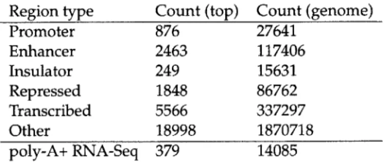
regions. Table 3.1 shows these counts for functional regions in GM12878 lymphoblastoid.

Only roughly 2,000 of these SNPs fall in enhancers, and even fewer fall in promoters and

transcribed regions. But this result raises another question: why do we have to traverse

30,000 SNPs in the ranked list before we pick up all of the 2,000 the enhancers which could

contribute to the enrichment. One potential explanation is we pick up SNPs in LD with

causal variants as we walk down the ranked list and therefore dilute the signal.

Region type Count (top) Count (genome) Promoter 876 27641 Enhancer 2463 117406 Insulator 249 15631 Repressed 1848 86762 Transcribed 5566 337297 Other 18998 1870718 poly-A+ RNA-Seq 379 14085

Table 3.1: Counts of top T1D-associated variants in functional regions in GM12878 lym-phoblastoid. In the top 30,000 variants, only a small fraction fall in promoters, enhancers, or coding regions (either predicted by chromatin marks or actually expressed).

3.2.2

Implicated enhancers appear genome-wide

This concern about LD is significant because regulatory regions are physically clustered. This fact follows naturally from the fact protein-protein interaction is the mechanism of transcriptional regulation. Proteins bind to sequence motifs in regulatory regions, which are close to each other either due to being close in terms of genetic (base pair) position or being close to each other in three-dimensional position (because the DNA molecule folds on itself). Variants which are nearby are in stronger LD and therefore their genotypes and p-values are more highly correlated The concern then is the 2,000 enhancers we find are all physically clustered and in LD with each other, so only a few of them are actually causal and the rest simply have correlated p-value.

Another concern is the enhancers we find all fall in the Major Histocompatability

Com-plex (MHC). Although genome-wide association studies consider mutations all over the

genome, the top p-values are often highly localized to the MHC. This region of the genome in chromosome 6 contains many genes related to the function of recognizing cell surface markers to distinguish cells belonging to oneself versus cells which are invaders. It is highly variable across individuals and human subpopulations due to its role in immune response. It also shows atypical LD patterns compared to the rest of the genome such as long-range LD (i.e., abnormally large blocks in which no recombination occurs). These features of the MHC violate usual assumptions used in GWAS statistical testing and there-fore variants in these regions often show highly significant p-values regardless of their relevance to the trait in question. Although in the case of T1D we expect to find hits in the MHC due to the autoimmune disease pathology, we also expect to find hits outside the MHC.

To visualize where in the genome the hits cluster, we map individual chromosomes

to Hilbert curves. Hilbert curves are space filling curves defined by David Hilbert in 1891

which map the one-dimensional line to the two-dimensional plane [5]. The key property of these curves we exploit is preservation of locality. If two points are close to each other on the line, they will remain close to each other when mapped to the Hilbert curve. Although the converse is not true (points which are far apart on the line may be mapped close to each other on the Hilbert curve), we are mainly concerned about overlaps which are close

.W~~SN 03nsitys,6h, d. h noyp

12000O0

8000I + +

000 0

toe oth1 e11 ch r.12 .14 0r10 1 111

82000 +4I0.

4000

~

arriti (R)aoher autoimmn disase Inded wefndalag lutrfrogl

12000 II

0 I

~

LL

Figure 3.4: Overlaps with GM12878 enhancers in the top 30,000 T D-associated variants and rheumatoid arthritis-associated variants mapped to Hnbert curves. No more than half the overlaps localize to the MHC (boxed). There are hundreds of independent clusters of enhancers, including some specific to each disease.

to each other.

Figure 3.4 shows this visualization for top enhancers in both TiD and rheumatoid

arthritis (RA), another autoimmune disease. Indeed, we find a large cluster of roughly

half the hits in the MIC. However, the remainder of the hits are scattered all over the

genome in small clusters giving further evidence these enhancers are independent.

More-over, while we observe many clusters are shared between the two diseases, we also find many clusters which are disease-specific. Although both TD and RA are autoimmune, they attack different parts of the human body (pancreas versus connective tissue). Ac-cordingly, disease-specific clusters of enhancers are potentially related to disease-specific disregulation which causes differential pathology

3.2.3

Implicated enhancers are independent of known associated loci

Another concern is the enhancers we find are linked by LD to known loci and therefore we are not actually finding novel associations. In the case of TD, 91 loci are listed in the TFDBase as reliably associated with the disease [33]. To address this issue, we subtract

out these loci (considering tagged SNPs with

r

_{.8) from foreground and background}

and redo the analysis. We address whether these enhancers are linked to nearby genes

by subtracting out TSS-proximal regions. We account for linkage to non-synonymous

variants by subtracting out loci tagged by those variants (again requiring

r

_{.8) We}

also do the same for loci overlapping the MHC.

Figure 3.5 shows we continue to find enrichment of enhancers even after subtracting

out all of these potential confounders, although to a lower magnitude. We continue to see separation of immune cell types from other cell types giving further evidence we are finding novel associations.

Minus T1 tc

0.3.

0.000125

5 75 037500 0 01 1 1500

o 3700 7r ao 11I I ;Soo 0 100

SNPs ranked by increasing p-value

Figure 3.5: Enrichment of enhancers persists after

such as known loci, nearby genes, coding variants,

tinue to be separated from other cell types even up

subtracting out potential confounders

and the MHC. Immune cell types

con-to 30,000 SNPs.

I1123 a 111 -ft

Figure 3.6: Generation of permuted enhancer tracks (orange) from real enhancer tracks

(blue). The permutation procedure samples from real elements and therefore preserves

their properties. Sampling is more likely to pick constitutive enhancers because they

ap-pear more often in the population of all elements, allowing us to investigate the

contribu-tion of these enhancers. We destroy the associacontribu-tion between the identity of the cell type

and which enhancers are assigned to it and hypothesize permuted tracks will show less

enrichment than real tracks.

3.2.4 Implicated enhancers are cell type-specific

Next, we look at whether the enhancers we found are actually specific to the immune cell

types or are constitutive (constant across all cell types). We first permute elements across

cell types to generate 100 new randomized cell types as shown in Figure 3.6. We first

sample a total number of elements from the distribution of total number of elements across

real cell types, then sample that number of elements from all elements across all cell types.

We hypothesize the identity of which enhancers are in a specific cell type is the important

quality. Therefore, our permutation procedure destroys this quality while preserving other

properties of the elements (such as the distribution of their sizes and distances to the closest

gene).

Figure 3.7 shows RR plots computed for these permuted cell types. We find all of

the randomized cell types show moderate enrichment early in the ranked list suggesting

this quantity is the contribution of constitutive enhancers. However, the enrichment is of

lesser magnitude than the observed enrichment for actual cell types. This result suggests

when we look at real cell types we are finding enrichment beyond

just

that of constitutive

Ir enh

J

Figure 3.7: Enrichment of permuted enhancer tracks. As in the case of promoters,

per-muted tracks show some enrichment in all cell types, suggesting they represent the

contri-bution of constitutive enhancers. However, the observed enrichment is less than that for

real enhancer tracks.

enhancers. Moreover, as in the case of promoters none of the cell types is separated from

the rest when considering enrichment of constitutive enhancers.

We next look at enhancer clusters. To perform the clustering, we sweep a line over

the concatenated genome. For each intersected enhancer, we take the union of enhancers

intersecting that enhancer across all the other cell types. For that region, we compute a

binary vector specifying whether the region overlaps an enhancer in each cell type. We

cluster these activity vectors using k-means clustering, iteratively picking optimal k. For

each cluster, we generate a new pseudo-cell type containing the regions corresponding to

the activity vectors assigned to that cluster.

Each cluster captures a set of enhancers which is specific to a set of cell types. Figure

3.9a shows for each cluster the cell types which the set of enhancers is active in. Red

indicates strong enhancer activity, orange weak, and purple poised activity. For example,

cluster 19 captures constitutive enhancers which are active in all cell types whereas cluster

5 captures enhancers which are active only in a small set of T helper and memory T cells.

Figure 3.8 shows the enrichment of these clusters for T1D-associated variants. We

find several clusters are enriched, showing clear separation from other clusters. As shown

in Figure 3.9b, the most enriched clusters are largely specific to immune cell types. One

cluster represents the contribution of constitutive enhancers and shows strong enrichment.

However, the cell type-specific clusters contain enhancers active in only two broad types

0.03 0.02-o ₁₆ 0.00 -0.01 037500 75000 112500 150000 SNPs ranked by increasing p-value

Figure 3.8: Enrichment of enhancer clusters for T1D-associated variants. Several clusters are clearly separated from the others. Moreover, we continue to see a greater magnitude of enrichment persisting to tens of thousands of SNPs.

of cells. The first are memory T cells, which recognize and respond to invasion. The sec-ond are T helper cells, which are initially programmable to respsec-ond to new invaders. After encountering a new antigen (cell surface marker which can be used to -identify invaders), they mature into either memory cells, effector cells which increase immune response when exposed to the same antigen, or regulatory cells which decrease immune response. Mis-classification of one's own cells and disregulation of the immune response at the tissue level are central to autoimmune disorders such as T1D. These results suggest we are in-deed finding enhancers which are specifically active in exactly the disease-relevant cell types. They could play a role in disregulation at the molecular level, modulating the ex-pression of important genes and function of important pathways which could give rise to the observed tissue-level disregulation.

3.2.5 Open chromatin is enriched for disease-associated variants

We have chromatin states for 9 ENCODE cell types and 85 Roadmap cell types. However, these cell types are still only a fraction of the full spectrum of human cell types. For other cell types we do not have this rich annotation of regulatory activity. However, for 90 dif-ferent ENCODE cell types we have experimental assays of open chromatin, another proxy for regulatory activity. Specifically, we have annotations of DNAseI hypersensitive sites (DHS) and Digital Genomic Footprints (DGF).

a

hESCDernied CD 84_ndcdem- CuredCell ES-WA7 Con Line

ES4-CaL Line PS-15bCeLine HUES4S CoOLinre

HUESB COI Line

IP5-18-CaItLine lPS-DbSCellLine HUESeOII *VLine PS DF 6._l6 el Lie HPSDF19 1_CelLine H BMP4 Deine lTellndodeeeCuturiedCob Gastric LePS 1 ele

Neurosphere _Cu m_Ce _sGanglin _Em nreDedv e.Doo HuFNSC 2

HershreCluilCls otx 8MH on ved.oo Hnpoat u SClo2_

BrainGermlnal Matdx.DonorHuFGM02 Hi Detalu Mll Fml toneyC Duodenum De MucosadDc n 61FCS Colonic Mucosa.DooM2 Feetallnsin.DnenoNSC2 Skeleta Muscle DStomachSmoth MusceDn

Rectals Mdie Donor 1 Adlpeoot-scle

BraineAnlete TmporaClLoe Bra id Fguae Grs Mes S hyrnal d las

ChdrcytsMroBn a m n _Con9 MscSte Ituell usdCela

PeNosForeskinelanocy en_Pdmaryn DnM u_skn

MobSiiredCD34_Primay_ D o r s0 5

llneinC_PdyCalls

CD4_C25+D TPd Cedol

BonaL wov -eiiveMese C D4m_MtemoryPrmry Cells CD4+_CD25-_dL17_PMA-lonomydn di1edMimdlMAuS ensclslte C qOCCustes

ln In MetF9nn lnle e

F u 39 isre_Ftoblasrizarnest atnoheii Ceros

Pels Fornesll aelndobta dtPr w , p ehyCees.D erkdrskinsO

PelsFoselLn llenlecytenletsny~e.Doite n 15

W r ps.Foenski-Me~nWWlmativeo.DrntneLmisss

T1 -asoied lSoeCl eie variant, wun ell fidoecntttvUlse. h tesso ciiym r specifical ien Denod Meimeuyneone Cell types

Mclz _ 34 fMs _c Sto rulaee Cells Pllns FnekleFlDeolsePnlnty Cel.Dn euneklei54 P obiliFed F n3lsP etyCels.nrAClnSS Pelsosln elenelluetoPr nnyCoDon nnRC ln10

CDSSPrlmoyColeG CD3_PrCdmareClls MolodC3 tnoyClDunnun 00 01502

I

CD+C2iL CD7_Co Pins syCells CdMnnyPlneany CellsA

CDinCDre 3L.9: PM-cneDn o e MCiedTactivty lloo ehne lutr.a roie cos l ls

Chie ees-lte PAnsey inuctive or1 P isn dana CaFcsnbo h o cutr nrce o

TlD-associate004 CvainLCts, wme P in ele Coleuiv lse. h ter h watiiym r specifcallyinPamune c ll ypes.

0.010 E 0 0025 0.020 0015-0 3700 75000 112500 150000 0 37500 75000 112500 15000 0 37000 75000 112500 150000

SNPs ranked by increasing p-value

Figure 3.10: Enrichment of open chromatin. Enrichment of DHS for T1D-associated vari-ants clearly separates immune cell types from others (left). The higher resolution DGF im-proves this separation (center). Intersecting DHS with ChromHMM enhancers imim-proves separation over just considering enhancers (right).

Figure 3.10 shows the enrichment of DHS and DGF for T1D-associated variants. Again we find T helper cells and CD20+ B cells are enriched. However, we find these cell types show greater separation from other irrelevant cell types. This result shows the importance of having annotations for the most disease-relevant cell types. Moreover, we find that the higher-resolution DGF annotation shows better separation between cell types, suggesting increasing the resolution of regulatory annotations will increase our power to detect regu-latory variants relevant to disease.

For a small number of cell types, we have both chromatin states and DHS, allowing us to further refine the annotation. By intersecting enhancer regions with DHS, we get regions which we are more confident have regulatory function. Indeed, we again find immune cell types are increasingly separated from other cell types.

All of these results point to molecular level regulation (i.e., regulation of gene expres-sion) as playing a role in Type 1 Diabetes. We find only enhancers in immune cell types relevant to T1D show enrichment for T1D-associated variants. This enrichment persists to tens of thousands of SNPs, suggesting the genetic architecture of T1D involves many more common variants than previously thought. We separate the contribution of these enhancers from the linked contributions of nearby genes and find it is indeed the regula-tory regions which are contributing to the observed enrichment. Moreover, we separate the contribution of constitutive enhancers from the contribution of enhancers specific to the enriched cell types. We find it is precisely those enhancers specific to disease-relevant immune cell types which show the strongest enrichment. Thus, these variants could con-tribute to molecular level disregulation, which in turn gives rise to tissue level disregula-tion of the immune response and the autoimmune disease pathology.