Characterization of whip targeting kinematics in discrete and rhythmic tasks

Characterization of Whip Targeting Kinematics in Discrete and Rhythmic Tasks

by Camille Henrot

Submitted to the

Department of Mechanical Engineering

in Partial Fulfillment of the Requirements for the Degree of Bachelor of Science in Mechanical Engineering

at the

Massachusetts Institute of Technology

June 2016

C 2016 Henrot. All rights reserved.

MASSACHUSETTS INSTITUTE OF TECHNOLOGY

JUL 0

8

2016

LIBRARIES

ARCHIVES

The author hereby grants to MIT permission to reproduce and to distribute publicly paper and electronic copies of this thesis document in whole or in part in any medium now known or

hereafter created.

Signature of Author:

Certified by:

_Signature redacted

Camille Henrot Department of Mechanical Engineering May 6,2016

Signature redacted

Neville Hogan Sun Jae Professor of Mechanical Engineering

Signature redacted

Characterization of Whip Targeting Kinematics in Discrete and Rhythmic Tasks

by Camille Henrot

Submitted to the Department of Mechanical Engineering on May 6, 2016 in Partial Fulfillment of the

Requirements for the Degree of

Bachelor of Science in Mechanical Engineering

ABSTRACT

Robotic control of complex objects is inferior to that of humans despite superior communication, sensors and actuators. Therefore, studying human control of complex dynamic objects, in

particular a bullwhip, should reveal how humans may achieve superior dexterity.

An expert whip-cracker performing two distinct targeting tasks, discrete and rhythmic, was observed using the Qualisys 3D motion capture software. The objective was to investigate the kinematics of the whip, the kinematics of the subject's arm while controlling the whip and the differences between discrete and rhythmic tasks.

The subject was able to expertly perform both targeting tasks with excellent targeting accuracy. The study confirmed the existence of a wave propagating down the whip as stated in prior work. Furthermore, a distinct difference between discrete and rhythmic tasks was observed in the reproducibility of position profiles, reproducibility of phase profiles, and the waveforms of elbow and wrist angles. Finally, the whip trajectory was substantially confined to a plane. In contrast with claims made in prior work, this plane was found to be distinct from the para-sagittal plane and slanted with respect to it.

Thesis Supervisor: Neville Hogan

ACKNOWLEDGEMENTS

The author would like to thank Professor Neville Hogan and Professor Dagmar Sternad for their support, guidance and mentorship throughout this research. It was a truly challenging and enjoyable experience which would not have been possible without their keen interest and engagement. Further thanks to Zhaoran Zhang for her knowledge and instruction in experimental design and analytical techniques and the Northeastern University Action Lab for lending their facilities and lab space. Special thanks to Adam Winrich for his bullwhip expertise, scientific curiosity and collaboration. Lastly, the author is truly grateful to Dr. Denis Henrot for his willingness to explore and discuss all facets of this work, and his unwavering fatherly coaching.

TABLE OF CONTENTS

1. IN TRO D UC TIO N ... 8

2. BA C KG R O UND ... 8

2.1 CRACKING A BULLWHIP ... 8

2.2 A SSUM PTIONS OF BULLW HIP KINEMATICS ... 10

2.3 INTRODUCTION TO DYNAMIC PRIMITIVES... 1

2.3.1 Subm ovem ents ... 11

2.3.2 Oscillations ... 11

2.3.3 M echanical Impedance ... 12

3. EX PER IM ENTA L SETUP...12

3.1 OVERVIEW OF SUBJECT AND EXPERIMENTS...12

3.1. 1 Subject ... 12

3.1.2 Experim ental Setup and M arker Placem ent ... 12

3.1.3 Experim ental D escription ... 14

3.2 QUALISYS 3D M OTION CAPTURE ... 15

3.2.1 D ata Acquisition...15

3.2.2 D ata Processing and Point Identification... 16

4. EX PER IM EN TA L M ETH O DS ... 17

4.1 DATA STRUCTURE AND INTEGRITY ... 17

4.1.1 D ata Integrity...18

4.1.2 D ata Structure and Segmentation ... 19

4.1.3 Testing Statistical Significance ... 20

4.2 CHARACTERIZATION OF W HIP KINEMATICS ... 20

4.2.1 Separation and Registration of Whip Trials ... 20

4.2.2 Whip Throwing Profile...21

4.2.3 W hip Velocity Profile ... 23

4.2.4 W hip Performance ... 23

4.3 CHARACTERIZATION OF A RM KINEMATICS ... 23

4.3.1 Elbow and Wrist Angle- Para-sagittal Plane... 23

4.4 CHARACTERIZATION OF SYSTEM KINEMATICS ... 25

4.4.1 Planarity D ata Subsets...25

4.4.2 Planarity - Least M ean Square Plane ... 25

4.4.3 Planarity - Principal Component Analysis... 26

4.4.4 D escribing a Plane in Spherical Coordinates ... 27

4.4.5 Position vs. Velocity Phase Profile ... 28

5. RESULTS ... 29

5.1 W HIP POSITION AND VELOCITY THROW ING PROFILES ... 29

5.2 TARGET ACCURACY ... 32

5.3 ELBOW AND W RIST ANGLE ... 34

5.4 PLANARITY ... 36

5.4.1 Characterization of Planarity using Least Mean Square and Principal Component Analysis .36 5.4.2 Least M ean Square Plane ... 37

5.4.3 Principal Component Analysis... 38

5.5 POSITION VS. V ELOCITY PHASE PROFILE ... 40

5.5.1 D ecomposed Phase Profile ... 40

6. DISC USSIO N ... 43

LIST OF FIGURES

Figure 1: Construction of a bullwhip (drawing from Conway [4]). ... 9

Figure 2: Examples of two common whip techniques (drawing from Conway [4])... 10

Figure 3: Experimental setup showing placement of subject and target. ... 13

Figure 4: Qualisys marker placement on subject and whip... 14

Figure 5: An example of one time sample of raw unidentified data in Qualisys Track Manager Softw are... 16

Figure 6: An example of one time sample of identified data in Qualisys Track Manager S oftw are... 17

Figure 7: Tree diagram showing the structure of data and data subsets... 20

Figure 8: Illustration of registration and segmentation process... 21

Figure 9: Graphic of throwing profile for rhythmic and discrete trials. ... 22

Figure 10: Elbow angle and distance between R5 and the target... 22

Figure 11: Elbow and wrist angle ... 24

Figure 12: Spherical coordinates showing cp, ( and r... 28

Figure 13: Position throwing profile for all whip markers in discrete and rhythmic tasks. ... 30

Figure 14: Velocity throwing profile for all whip markers in discrete and rhythmic tasks... 31

Figure 15: Minimum distance between target and whip points in discrete task... 32

Figure 16: Minimum distance between target and whip points in rhythmic task... 33

Figure 17: Mean and standard deviation of minimum distance between target and whip points.33 Figure 18: Elbow and wrist angle of three trials in discrete task... 35

Figure 19: Elbow and wrist angle of three trials in rhythmic task... 35

Figure 20: Comparison of LMS and PCA cp and 0 values... 36

Figure 21: Normalized average root mean square error of LMS plane fit for discrete and rhythm ic tasks... 38

Figure 22: Relative eigenvalue contribution of principal components for shoulder to R5 markers in discrete and rhythm ic tasks... 39

Figure 23: Angle standard deviation of principal component direction from mean direction of all w hip points R 1, R2, ... , R5... 40

Figure 24: Position and velocity phase profiles for discrete and rhythmic tasks. ... 41

Figure 25: Normalized position and velocity phase profiles for discrete and rhythmic tasks... 42

LIST OF TABLES

Table 1: Data occurrence cases. A 1 represents that marker data existed for that sample. A 0 represents that marker data did not exist for that sample... 18 Table 2: Whip marker case occurrence percentage for all discrete and rhythmic trials... 19 Table 3: Data subsets used in two methods of planarity analysis. Sets of ten trials were used for each calculation... 25 Table 4: Average thickness of position profiles in discrete and rhythmic whip tasks... 30 Table 5: Average thickness of velocity profiles in discrete and rhythmic whip tasks... 32 Table 6: Average minimum distance between target and points on the whip. These values are compared to physical distances between markers measured in the experimental setup shown in row three. ... 34 Table 7: Full whip (Ri, R2, ... ,R5) planarity comparison between discrete and rhythmic tasks and comparison of LMS, PCA and para-sagittal planes... 37 Table 8: Relative contribution from each principal component. Values are in percent of total variance for each m arker... 39 Table 9: Average eigenvector for each principal component for whip markers RI, R2, ... , R5 in

1. Introduction

A challenge of robotic control is understanding and emulating the simplicity by which humans do what they do. How can a robot or a piece of machinery imitate human dexterity? The paradox remains that human communication, computation, and actuation are vastly slower than most modem robots, yet humans achieve dexterity superior to robots. Studying human control of complex dynamic objects should reveal how humans achieve superior dexterity.

Some theories of human neural control state that when humans come into contact with objects, the central nervous system back-calculates a kinematic model and predicts the exact mathematical behavior of the object [1]. Hogan and Stemad, on the other hand, suggest that this dexterity, instead, arises from encoding motor commands as dynamic primitives [1]. Dynamic primitives suggest a different neural representation of complex object manipulation. Two such primitives are rhythmic and discrete motions: a rhythmic motion is periodic while a discrete motion is a stand-alone motion in time.

One particularly complex dynamic object is a bullwhip. The bullwhip varies in both diameter and flexibility along its length and the physical phenomenon of cracking a whip requires parts of the whip to exceed the speed of sound. However, experts can reliably 'crack' a whip or use it to strike small targets from large distances.

This project studied the performance of an expert whip user striking an object of 5cm diameter from a distance of 1.8m, which was done for both rhythmic and discrete execution.

Most historical research regarding bullwhips explores mathematical modelling and the exact motion of the whip; however, we found no discussion of the interaction between the human and the bullwhip [2,3]. Prior work has studied the character of the crack of the whip and the trajectory of the whip during a crack. This study instead focused on the targeting task analyzing control, consistency, and reproducibility of the whip trajectory. The characterization of the motion of an expertly controlled whip can be used as a foundation for further work in the study of complex dynamic object control.

2. Background

2.1 Cracking a Bullwhip

According to Goriely, the representation and use of whips is widely misunderstood not only in research circles but in broader communities as well [2]. In fact, the bullwhip is one of the most interesting objects from the standpoint of complex object manipulation. The main purpose of the bullwhip is to produce a distinct, loud cracking sound, used initially to direct animals as well as for communication purposes. Nowadays bull-whip manipulation has become a source of entertainment for wide audiences.

A common bullwhip is made out of a heavy, robust material such as leather or nylon. A detailed schematic is shown below in Figure 1. The whip is made of two parts: the handle and the thong. The handle is the widest and most rigid part of the whip, while the cracker, on the tip of the thong, is the thinnest and most flexible. The crack occurs as the cracker reaches supersonic speed.

thong

le (insde whv

Figure 1: Construction of a bullwhip (drawing from Conway [4]). The

handle is rigid, the thong is flexible and the cracker, at the end of the

whip, is responsible for the distinctive cracking sound.

Goriely and Bernstein both focus specifically on the production of a cracking sound in their studies. The most common explanation of whip motion is that an abrupt change in tension

creates an initial waveform propagating down the length of the whip from the handle to the tip of the cracker [2,3]. _{As the bullwhip diameter decreases down the length of the whip, the velocity}

increases and eventually exceeds the speed of sound [5].

Goriely points out that most studies explaining the cracking phenomenon of whips assume a specified shape of the whip over time [2]. The model for the shape of the whip is fairly complex and depends on many factors such as the initial formation of a loop, boundary

conditions (initial handle velocity and subsequent free-end velocity), whip construction (the effects of tapering) and tension in the whip. Furthermore, for each distinct whip-cracking or targeting technique there exists a different transient whip shape though each technique still produces the cracking sound.

There are several techniques for whip cracking, however the two most common are the forward crack and the cut or overhand technique, often used for targeting [2]. Both techniques are visualized below in Figure 2. The forward crack is neither the most intuitive nor the most efficient technique to crack the whip but it is the technique showing the most obvious wave propagation down the flexible thong. The cut or overhand technique, generally used for targeting, is based upon a change of direction of the whip at the top of the arm motion. The whip-cracker swings the whole whip up off the ground and suddenly changes direction of the handle to produce a rolling shape that propagates as a wave [4]. This project singled out targeting tasks using the cut overhand technique.

(A)

(iv)

Yb,

4,

(v) (vi)

(B)

(i) (ii) (iii)

Figure 2: Examples of two common whip techniques (drawing from Conway [4]). (A) forward crack technique and (B) cut overhand technique. The cut overhand technique was used in all experiments in this project, the subject swings the whip of the ground (i), reverses ann motion (ii), and the whip cracks over the hand and forward (iii).

2.2 Assumptions of Bullwhip Kinematics

The body of prior bullwhip research focuses heavily on the cracking phenomenon. It would appear that the cracking sound is simultaneous with the targeting task. In this regard, the assumptions made in the study of whip-cracking are relevant to targeting tasks.

One kinematic assumption of whip-cracking research is that all whip motion remains planar. This means that at any point in time the trajectory of the whip in 3D space can be reduced to a two dimensional kinematic system [6]. Generally, the plane is assumed to be in the

para-sagittal plane, the vertical plane beside the body, or the overhead plane depending on the technique being used.

An excellently crafted whip is constructed with fine cross-hair braiding such that it is possible for an initial planar shape to remain planar as it propagates down the whip [4]. Of course, this behavior is dependent on the skill and dexterity of the manipulator along with the construction of the whip. For example, it may be more difficult to maintain a planar whip trajectory with a poorly constructed whip, in the same way that it may be more difficult for a novice whip user to maintain whip planarity. This project explored planarity in whip targeting

tasks for an expert whip user. It defined the degree of whip planarity as well as the plane that described the trajectory of the whip.

2.3 Introduction to Dynamic Primitives

Recent work has shown that there is a large distinction in neural control between discrete and rhythmic motions that support the need for the theory of dynamic primitives [7]. It is highly unlikely that the central nervous system computes an exact internal model of human motion when in contact with a complex object for example, a whip. If this were not the case, then the human would be able to control the same object in the same way regardless of discrete or rhythmic tasks. This is the motivation for dynamic primitives.

A study by Schaal shows that discrete and rhythmic motions elicit not only different cerebral activation but that, in fact, there are distinctly measurable transitions that occur between discrete and rhythmic motions as the speed of a discrete task is increased [8,9]. This project explored the differences between discrete and rhythmic motion.

Hogan and Sternad propose that the human interactive behavior is composed of at least three dynamic primitives: submovements, oscillations and mechanical impedances [10]. Of the three, impedance is specifically relevant to the use of tools. These dynamic primitives need not be mutually exclusive and, in fact, it is their simultaneous existence that allows for such complex movements to be so easily performed and retained by the user [10]. It is important to note that humans can voluntarily control all three types of dynamic primitives.

Though this project is not specifically focused on dynamic primitives, the final goal of this study is to gain an empirical understanding of the dynamic primitives at play with whip use. The existence and subsequent definition of dynamic primitive interaction and superposition in whip use is useful in further defining the observed dexterity of humans and to eventually apply such primitives to the field of robotics.

2.3.1 Submovements

Submovements are like discrete movements in that, alone they are movements that begin and end at rest. However, in the case of human dexterity these submovements are stand-alone motions that can then be superimposed in time with other dynamic primitives. Hogan and Sternad define a submovement as "a smooth sigmoidal transition from one value to another with a stereotyped time-profile" and that "each coordinate's speed profile has the same shape which is non-zero for a finite duration" [1].

2.32 Oscillations

The oscillatory primitive is described as an almost periodic-motion. The main distinction is that oscillations are not made up of many overlapping submovements in opposite directions. Though amplitude and exact behavior of the oscillation may vary over time due to fluctuations of biological systems, the average time course of oscillatory behavior is periodic. This periodic behavior should have the same shape for it to be considered an oscillatory dynamic primitive [1].

2.3.3 Mechanical Impedance

Mechanical impedance is the dynamic primitive that deals most with contact and interaction that humans encounter in their daily activities. Fundamentally, cracking a whip requires a mechanical interaction between the manipulator and the whip itself. This interaction is generally an impedance, a generalized stiffness, that specifies the force response to the motion of the object or environment [11]. It should be noted that control of interaction and contact with objects can drastically change the dynamics of a system, often changing its order and

complexity. However, mechanical impedance is solely a result of the neuro-mechanical system and is not changed by the presence of contact or interaction, making it an extremely robust method of motor control [10].

3. Experimental Setup

Two experiments were performed to assess the position, velocity, and planarity of both the subject's arm motion as well as the whip trajectory when using the whip to hit a target. Using

the Qualisys 3D motion capture system, three-dimensional positions were recorded for markers

along the whip and markers on the subject's arm for each targeting task.

3.1 Overview of Subject and Experiments 3.1.1 Subject

One male right-handed expert whip-cracker with more than 15 years of whip-cracking experience participated in experiments 1 and 2 after giving informed consent. All experimental protocols were approved by the Institutional Review Boards (IRBs) of the Massachusetts Institute of Technology on the use of human subjects in research. Extensive work in target-oriented whip tricks as well as national and international competitions made this subject representative of controlled whip motion and expert whip manipulation.

3.1.2 Experimental Setup and Marker Placement

The subject performed two whip-cracking tasks: discrete and rhythmic execution. The goal of both tasks was to hit or touch a spherical target mounted on a spring with the tip of a 6ft bullwhip. As shown in Figure 3, the subject was positioned six feet, 1.83m, away from the target to ensure that the end of the whip would hit the target. The target was oriented at the center of the subject's chest at 60% of the subject's height, such that the target was in line with the subject's hand.

The position of the target was calibrated before trials began, namely (x, y, z) of the target was determined before any targeting attempts. In some cases, the fast velocity of the end of the whip displaced the marker from the target making the target unmeasurable (the marker was no longer in the measurable volume of the motion system cameras) for the rest of the session. Through target calibration, success of each trial was assessed by verifying the distance between the calibrated target position and the position of the last marker on the whip.

h

0.6h

1.83m

y

Figure 3: Experimental setup showing placement of subject and target. The subject is positioned 1.83m from the target. The target is positioned at 60% the subject's height. The x direction is across the subject's body, the y direction is towards the target and the z direction is vertically upward from the ground.

To measure position of the subject and the whip, retro-reflective markers were attached to the subject's dominant arm (right arm), trunk, and head using double-sided adhesive tape

designed to be applied directly to the skin. Smaller markers were attached along the length of the whip in six positions. Each position along the whip had two markers placed opposite to each other on the circumference of the whip. This was done to maximize the probability of

measurement at every location. No markers were attached to the very end of the cracker of the whip, as there was no physical support available and it would have drastically changed the kinematics of the very thin cracker string. The marker placement on the arm and whip can be seen in Figure 4 below.

The handle of the whip, in this case, was considered rigid while the rest of the markers were attached to flexible portions of the whip. Due to the construction of the whip, the flexibility of the whip increases down its length. As a consequence, marker R6 is located on a more flexible area of the whip than marker RI.

R6 R5

Marker Marker Placement Symbol

Code

HEF Front of the head

HEB Back of the head

CLAV Clavicle, between collar bones

STRN Sternum, base of rib cage 0 C7 C7 bone at the top of spinal column t Ti0 Tenth vertebrae on spinal column

RBWT Right back waist LBWT Left back waist RFSH Right front shoulder

RBSH Right back shoulder 0

RIEB Right inner elbow

ROEB Right outer elbow 0

RWR Right wrist RHA Right hand

R4 R3 R2 R1

- --- -

-45 cm 33 cm 33 cm 29 cm 27 cm 24 cm

Figure 4: Qualisys marker placement on subject and whip. The markers were placed on the head trunk and dominant arm of the subject. 6 markers were placed down the length of the whip, RI referring to the marker closest to the handle and R6 closest to the tip of the whip.

3.1.3 Experimental Description

The goal of each task was to hit or touch the spring target with the end of the whip. In the discrete case, the subject was instructed to perform 5 sessions of 20 discrete whip targeting attempts, totaling to 100 discrete trials over all sessions. The subject was verbally cued to begin each discrete attempt with a "go" signal and proceeded to choose the speed with which he manipulated the whip. Once the subject finished one attempt (trial) he was instructed to come to rest until another cue was given. In rhythmic execution, the subject was instructed to perform 2 sessions of 50 continuous whip trials. However, in the second session the subject did 51

subject was cued to begin with a "go" signal and was self-paced in 50 continuous trials without rest. On the fiftieth trial the subject was cued to stop.

In both executions the subject was considered successful if he hit the target. There was visual feedback as the target would oscillate when it was hit. In discrete execution, if the subject was successful, he was instructed to stay at rest until the target oscillation was fully damped. In rhythmic execution, if the subject was successful, the target was not damped and the subject continued to attempt to hit the target. In some cases, the cracker of the whip got caught on the target (discrete: 10 trials out of 100, rhythmic: 1 trial out of 101). These trials were recorded but the data was not included in subsequent analysis. In total, there were 90 valid discrete trials and 100 valid rhythmic trials used in our data analysis.

3.2 Qualisys 3D Motion Capture

Data acquisition consisted of two main parts. The first was 3D motion capture, using the

Qualisys motion capture system. The second was identifying markers in each trial using Qualisys

Track Manager Software.

3.2.1 Data Acquisition

Traditionally, whip dynamics are studied by means of two-dimensional data acquisition systems such as high-speed video and high-speed shadow photography [2,3]. High-speed video is a robust method to measure and understand transient behavior of complex objects; however, this project explored a new method of 3D data acquisition.

The Qualisys motion capture system is a series of 12 infrared optical cameras. The

cameras emit a ray of infrared light which is then reflected by the retro-reflective markers attached to the subject and the whip. The information from these markers is then used for 3D reconstruction of the markers in space [12].

The system must first be calibrated to determine the field of view of this composite camera where marker position can be measured. The calibration process used the Qualisys calibration wand and an axes frame on the ground of the space. The x axis was the direction across the subject's body, the y-axis was direction between the subject and the target and the z-axis was vertical from the ground. Calibration took about 20 to 30 seconds. The field of view of the experimental space was swept with the calibration wand. The Qualisys Track Manager

Software automatically determined whether the calibration was successful or if another calibration process is required.

Once the system was calibrated, the subject and whip marker positions could be measured. Data were recorded with a sampling rate of 200 Hz for up to 3 minutes, so about 3.6 x 10' time samples per trial. Once recording began the movement of the subject and the whip was recorded until the recording was stopped manually.

Figure 5 below shows an example of the raw data captured in a trial. Initially the data is unidentified, meaning all data are raw position measurements, not linked to any particular marker.

Figure 5: An example of one time sample of raw unidentified data in Qualisys Track Manager Software. The red points in space are unidentified markers corresponding to the markers on the subject and the whip. The x axis is denoted by a red arrow, y axis, light blue and z axis dark blue. The two rectangles on the ground are force pads that were not used for this experiment.

3 .2 .2 Data, Processing and Point ldentificatWn

While the track manager software can accurately measure all markers in the field of view, the software does not automatically define what each marker is, i.e. shoulder vs. RI. In order to extract data for each marker, one must identify the measured markers with useful headings or names. This point and click data processing technique is prone to human error.

The fill level of a marker refers to the percentage of time relative to the whole trial the

particular marker is seen by the cameras. If a point is obscured during the trial this will be shown

in a lower fill level. At any time when a marker is obscured the marker must be re-identified.

In the case of the markers on the subject, the fill level was generally I 00% and relatively

simple to identify. However, in the case of the markers on the whip, many were obscured due to

the kinematics of the whip in space, resulting in a much lower fill level. Over the course of each

trial most whip markers required some amount of re-identification. This is where the redundancy of markers became helpful.

Figure 6: An example of one time sample of identified data in Qualisys Track Manager Software. The colored points in space are examples of identified data. Green points correspond to markers on the subject, while the other colors correspond uniquely to a whip marker Rl, R2, ... , R5. Visual distinction in the identification process is useful to decrease possible error. The x axis is denoted by a red arrow, y axis, light blue and z axis dark blue. The two rectangles on the ground are force pads that were not used for this experiment.

Once markers were identified, the data was segmented into individual trials. Subsequent data processing was performed in Matlab.

4. Experimental Methods

The data acquired in the two experiments required several analysis techniques to

characterize controlled whip motion. Through the following experimental methods whip and arm kinematics were characterized through position profiles, velocity profiles, joint angles, and planarity studies.

4.1 Data Structure and Integrity

Part of this project explored a new method of data acquisition to study whip motion. Through multiple data acquisition and troubleshooting trials, we developed a robust data capture methodology. This particular set of data required specific processing and restructuring to enable the analysis.

41.1 Data Integrity

Though the Qualisys system is a highly sophisticated system, it still requires manual processing to ensure the integrity of the data, particularly in the case of capturing whip motion. The markers used on the whip were small retro-reflective spheres that were attached to the whip with adhesives. These markers are quite fragile and due to their small size can easily be obscured during data acquisition. One objective of this experiment was to design a data acquisition

protocol such that the data of whip motion would be adequate to sufficiently describe the motion in the experiment.

An important design feature was marker redundancy. On each measurement point along the whip, two Qualisys markers were attached. This was to increase the probability of

measurement of that particular point on the whip during each trial. For this reason, for each sample in a trial there are four distinct cases of marker data, detailed in the Table 1 below. An entry of 1 represents the existence of data for that sample, while an entry of 0 represents no data for that sample.

Table 1: Data occurrence cases. A I represents that marker data existed for that sample. A 0 represents that marker data did not exist for that sample.

Marker 1 Marker 2 Analysis

The resulting whip point data for time point t is

Case 1 1 1 the arithmetic mean in x, y and z position of the

markers.

Case 2 1 0 The resulting data for time point t is the raw x,

y and z position data from marker 1.

Case 3 0 1 The resulting data for time point t is the raw x,

y and z position data from marker 2.

There is no data available thus, the resulting

Case 4 0 0 whip point data for time point t, is not a

number (NaN) and results in a hole in 3D

position data for that trial.

Table 2 shows the percentages of case occurrences for each whip marker over all trials in both rhythmic and discrete tasks. It shows which points on the whip were most measured and which points on the whip were least measured. Whip point R6 did not result in a full data set in either discrete or rhythmic tasks. For this reason R6 data in particular was discarded in the analyses.

Table 2: Whip marker case occurrence percentage for all discrete and rhythmic trials.

Case 1 Case 2 Case 3 Case 4

Whip Discrete Rhythmic Discrete Rhythmic Discrete Rhythmic Discrete Rhythmic

Marker (%) (%) (% % (%) (%) (%) (%) RI 8.17 19.43 72.66 69.56 9.06 9.97 10.11 1.03 R2 2.75 16.71 88.96 64.12 2.81 17.06 5.48 2.10 R3 31.53 58.99 47.27 28.24 20.30 12.23 0.90 0.55 R4 2.34 11.32 60.33 64.10 1.07 14.62 36.26 9.96 R5 8.47 27.68 40.98 60.35 8.89 8.14 41.54 3.82 R6 0.00 0.00 7.92 19.56 0.00 0.00 92.10 80.44

In retrospect, marker redundancy was quite useful to ensure data integrity. As can be seen the occurrence rate for Case 1 in all whip points is much lower than the combined occurrence of

Case 2 and Case 3, showing that at any time point t, it is quite unlikely for both markers to be measured by the Qualisys system. When identifying points in the track manager system, there is no practical way to distinguish between marker I or marker 2, one can only distinguish if the point is RI, R2, R3 etc. In this sense, Cases 2 and 3 are examples of a similar case where only

one marker is visible.

Clearly, there are improvements to be made in this procedure. Firstly, the positioning of the cameras makes a great deal of difference and therefore should be optimized for future whip experiments, particularly for the trajectory swept out by markers further down the length of the whip. However, due to the nature of this data acquisition method, the processing of data is critical to the analysis. Redundancy of measurement points, organization and processing of case

occurrences are all integral to the data integrity required for characterization of the whip motion.

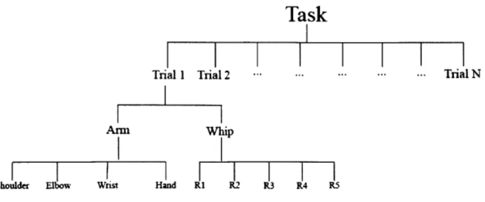
4.12 Data Structure and Segmentation

For clarity in subsequent sections, the structure and format of the data are detailed in Figure 7 below. Each task, rhythmic and discrete, has a set of data. These data were separated into trials, each trial being a whip attempt to hit the target. For the discrete task, the data included 90 trials and for the rhythmic task, the data included 100 trials. Within each trial there are two main data subsets. The first is the full whip and the second is the arm. The arm data includes position data of the shoulder, elbow, wrist, and hand. While the full whip includes position data

for markers RI, R2, ... , R6. However, R6 was discarded for reasons explained above.

The data were initially organized by each individual trial or whip attempt. For each whip attempt (x, y, z, t) were stored in a data set. Using Visual3D software, each trial for each marker was pipelined such that each marker had a data structure of n trials and each trial had (x, y, z, t). Each trial was cut manually in Qualisys Software using a reference position to define initial and final sample of each trial. However, as the subject controlled the speed of each trial, the lengths of the trials were usually different.

Task

Trial 1l Trial2 TriN

Arm Wip

Shoulder Elbow Wrist Hand Ri R2 R3 R4 R5

Figure 7: Tree diagram showing the structure of data and data subsets. There were two tasks: discrete and rhythmic. Most data analysis was applied horizontally across trials or subsets of trials. Each trial has subsets of arm versus whip data, and each of these sets includes multiple data markers.

Most data analysis was applied horizontally across trials, that is that the analysis was applied to each individual trial and then averages were taken over collections of trials. An alternative approach was to analyze a subset of trials and average across all subsets.

41.3 Testing Statistical Significance

To test hypotheses of possible relationships between discrete and rhythmic tasks as well as between neighboring whip markers, one-tailed t-tests were used with an alpha value of 0.05. Statistical significance was calculated on large data sets of average values to test the probability of a relationship between two data sets.

This method was used to estimate the probability that the observed relationships were due to random occurrence. If the probability is calculated to be below the alpha value, the null

hypothesis- there is not relationship between data sets- is rejected and the experimental hypothesis accepted [13].

4.2 Characterization of Whip Kinematics

One main objective of both experiments was to characterize the motion of the whip as controlled by the expert whip user. We characterized the kinematic behavior of the whip focusing on reproducibility, performance rating, position and velocity profiles. Discrete and rhythmic executions were analyzed separately in each of the following sections.

4.2.1 Separation and Registration of Whip Trials

In order to analyze position and velocity profiles over many trials, each set of trial data had to be matched to a common reference point and be of the same array length. Figure 8 shows the segmentation and registration process. To compare data across trials, a reference point, P,,, the maximum peak value of RI z-position for each whip trial n, and its corresponding time

index, I,,, were used to match trials. Each trial had a length of elements before I, defined as L, and a length of elements after I,,, defined as Lf. The minimum L, and Ljacross all whip trials were chosen as the final matching length for all trials. For each whip trial the start index was

calculated as (I, -_{Li""") and the end index was calculated as (If+L""). In this manner, all whip}

trials for all markers along the whip were matched at peak point P with equal array length.

( )1.8 T__ T- ril1 (A) 1.6 18 Trial 20 -Tria 21 1.4- Trial 22 E c 1.2 -o 02 1-0.8 0.6 -0.4 0 100 200 300 400 500 600 700 800 Time Samples (B)-1.6 T 1.4 Tra2 E 1.2 1-N0.8 0.6-0.4 (In-L """) Ini~" 200 300 400 500 600 700 800 900 1000 1100 Time Samples

Figure 8: Illustration of registration and segmentation process. (A) raw trials before registration, (B) trials after registration.

42.2 Whip Throwing Profile

To further compare discrete and rhythmic tasks, the data was segmented again such that it only included the throwing motion of the whip. The throwing motion was part of both discrete and rhythmic tasks, however, the tasks differed in the rest of each trial. In discrete trials the arm and whip came back to rest at the side of the subject, whereas in rhythmic trials the arm and whip continuously cycled through throwing motions. In order to compare the targeting differences in the two experiments, data was segmented into throwing profiles.

Figure 9 shows a diagram of the throwing profile. A throwing profile was defined to begin when the elbow angle was at a minimum and end at the instant when R5 reached a minimum distance from the target. The minimum distance between R5 and the target is the instant where the success or failure of each trial was determined.

R2 R3 R4 R5

R1 R2R 5 Target

Minimum Distance

Minimum _R5-Target

Elbow Angle

Figure 9: Graphic of throwing profile for rhythmic and discrete trials. The profile begins at the time of minimum elbow angle and ends at the minimum distance between the target and R5 in each trial.

Figure 10 illustrates the profile waveforms of the method above.

c2

0 u.J

(9

Throw Profile Indexing - Discrete

I/, I I I I I I I I 1.0 2.0 3.0 Time (sec) Z) ~0 Cz Ct 2cc 4.0

Throw Profile Indexing -Rhythmic

1.0 2.0 Time (se C) H V C) C) .0 C) 3.0 4.0 5.0 c)

Figure 10: Elbow angle and distance between R5 and the target. Black dashed lines designate the beginning and end of the throwing profile.

~1 0 -M Ui U-5

0

42.3 Whip Velocity Profile

The second characterization of whip kinematics is the average velocity profile for all points along the whip over all trials. In most cases, if data was missing the missing portion would be a group of 5-10 time samples, not just one time sample. Therefore, the velocity slope

calculation needed a sufficient range of samples. Given a position value at time point i and a range of position values from time points i-5 to i+5, the velocity is calculated as a slope using neighboring points, per Equation 1, to account for any missing data due to earlier point

identification. This method maximized the number of velocity estimates available. Velocity was calculated using the following equation:

i (ti - )x(x-)(

Zi= _{i (ti - T~)x(ti - F)}

In this case, E and i are the mean values of time and position in the range.

4.2.4 Whip Performance

Another method to characterize whip motion is through a metric of the subject's whip performance over many trials. The subject's whip targeting performance was quantified in terms of the position of all whip points measured relative to the calibrated target position.

In each trial, the minimum distance between each point on the whip and the target was calculated to show a performance metric for the whip motion. The minimum distance

calculations were unreliable for the performance of R6 as the marker was not measurable in close proximity to the target itself.

As the integrity of target and R6 data was not adequate to get a direct calculation of performance, target accuracy was extrapolated based on the physical distance between R5 and the tip of the whip cracker. Target accuracy for discrete and rhythmic tasks was calculated using the following equation.

minimum distance R5-Target (2)

physical distance

Minimum distance between R5 and the target was calculated by averaging the minimum distance over all trials. Physical distance refers to the measured distance between R5 and the tip of the cracker from the experimental setup.

4.3 Characterization of Arm Kinematics

4.3.1 Elbow and Wrist Angle- Para-sagittal Plane

approximation should be sufficient to understand the transient behavior of the elbow and wrist during whip trials.

(xs, Ys, ZS)

(Xe, Ye, Ze)

-- - -(x , yW, zw)

Xe, Ye, Ze) 01 (Xh, Yh, Zh)

-- ---- -- - Y--

(xw, yW, ZW)

Figure 11: Elbow and wrist angle. The elbow angle 0

ebow, is shown in blue and the wrist angle Owrist, is shown in orange. The other angles are required by the calculation process below. Blue and orange circles represent the markers on the subject during experimentation.

For elbow angle calculation

Cos 01

(

1(Vs

+ (z, - Ze)2

CoS 62 =( Yw - Ye

2 d(Yw ye)2 + (z, - Ze)2

eelbow = 61 - 02

For wrist angle calculation

Cos 1 =

(

I

4.4 Characterization of System Kinematics 4.4.1 Planarity Data Subsets

For all planarity analysis, the data was organized into subsets of ten whip trials, outlined in Table 3. For discrete and rhythmic tasks, there were 9 and 10 calculation subsets respectively. The subsets of data analyzed were identical in both methods.

Table 3: Data subsets used in two methods of planarity analysis. Sets of ten trials were used for each calculation.

Method Trial Subsets

LMS Discrete 1-10, 11-20, ... , 81-90

Rhythmic 1-10, 11-20, ... , 91-100

PCA Discrete 1-10, 11-20, ... , 81-90

Rhythmic 1-10, 11-20,..., 91-100

4.4.2 Planarity - Least Mean Square Plane

In historical work, the whip trajectory has been assumed but not proven as planar. There are three possibilities for planarity: each individual point's trajectory is confined to its unique plane, or all point's trajectories belong to the same plane, or there are multiple planes in the

system shared by various groups of points along the whip.

To determine planarity, a plane was fit to the throwing profile for each individual whip trial using the Least Mean Square (LMS) method. This Least Square planar fitting method assumes that the z-component of the data is dependent on the x and y-components. Due to this assumption, planarity was also confirmed using a secondary method.

Given the data set: {(xi, yi, zi)} L1

The plane was parameterized as follows

z = Ax + By + C (9)

The values of A, B and C are determined to minimize the mean square error Error is calculated by

n ₍₁₀₎

E(A, B, C) [(Axi + Byi + C) - zi2

This error function is non negative and its minimum, the least square value, occurs at:

n ₍₁₂₎ (0,0,0) = VE = 2 [(Axi + By + C) - z;] (xi, y1, 1)

i=1 Which leads to the matrix equation

=1 x1? L=1 xiyi ',=1 xi" A' =1 xizi (13)

L~=

X

Y

Y1

XL=1Y

[y

J

B

V

Y2ii

2L=1 xi 1= y L~=1

]1

Solved by matrix inversion and subsequent multiplication [14].

By construction, A, B, C are the coefficients of the plane satisfying the LMS error criterion. Furthermore, the LMS error can serve as a figure of merit for planarity of the whip trajectory.

Each error value was normalized by the total distance travelled for individual whip markers. Larger travelled distances are less likely to fit to a plane, therefore one would expect the error value to increase for each marker down the length of the whip. Normalization allows for an unbiased calculation in this regard.

RMSE (14)

Normalized Error (%) =

distance travelled

The normalized error is thus a percentage value of the total distance travelled. A smaller percentage corresponds to a higher degree of planarity.

4.4.3 Planarity - Principal Component Analysis

Principal Component Analysis (PCA) provides insight into the dimensionality of data. In this case, we are interested in whether the whip trajectory data set is approximately confined to a plane or a line.

PCA consists in determining eigenvectors and eigenvalues of the covariance matrix for a data set. The covariance matrix is a multi-dimensional generalization of the concept of variance. For two dimensions covariance is calculated as follows,

)

=₁(x -:0x(yi -Y) (15)

(n -1)

For our three dimensional case the covariance becomes a real-valued symmetrical matrix of size 3x3 where the diagonal values are the variances in x, y and z directions.

cov(x,x) cov(x,y) cov(x,z) (16)

C = cov(y,x) cov(y,y) cov(y,z)

For a three-dimensional data set, three eigenvector, eigenvalue pairs are then calculated. Each eigenvector is a direction while the eigenvalue translates the amount of data variability in that direction. As the covariance matrix is real-valued, positive-definite and symmetric, the eigenvectors are orthogonal. The eigenvector corresponding to the biggest eigenvalue (first principal component) provides the direction in which the data shows the highest degree of variability. For a data structure to be considered planar, two eigenvalues would be much greater than the third. For a data structure to be considered linear, one eigenvalue would be much greater than the other two eigenvalues. If all eigenvalues have comparable magnitude, there is no

underlying data structure and hence reduction of dimensionality of the data set is not possible [15]. Note that, equal eigenvalues are equivalent to an isotropic distribution of the data in space.

In terms of analyzing eigenvectors, standard deviation of principal component direction was calculated for discrete and rhythmic tasks. For each whip marker the average direction was

calculated. Similarly, for all whip markers RI, R2, ... , R5, the average direction was calculated.

The angles between the five whip marker direction vectors and the average direction of all whip markers were calculated.

V = [X,y,Z]R _{1 (17)}

W = [X, Y, Z]R1,R2,...,R5 ₍₁₈₎

_ _- _ 1 (19)

.6 = CoS~'iiiiiii

Standard deviation of each principal component direction was thus the standard deviation of the five calculated angles for discrete and rhythmic tasks.

4.4.4 Describing a Plane in Spherical Coordinates

To compare results from LMS and PCA, the planes were represented in spherical

coordinates. By defining the normal of the plane from a (0,0,0) origin, the plane's orientation can be described by what we will define as the attitude, (cp, 0), see Figure 12. T>, is generally

Z

0(,

6,<P)

X

Figure 12: Spherical coordinates showing q>, E) and r. 0 is defined as the polar angle and c) is the azimuth angle. We will refer to (q>, ()) as the attitude of the plane. [ 16].

The para-sagittal plane has an attitude of (q>, E))= (0, 90) degrees. Any deviation from these two angles shows a deviation from the para-sagittal plane.

4.4.5 Position vs. Velocity Phase Profile

If the kinematic behavior arises from a state-determined system, it may be represented as (D =<(q) where q is a vector. For a second-order system, a phase plot of 4 vs. q displays the

system dynamic equations. A position versus velocity plot is similar to a phase plot; a geometric representation of a dynamical system in state space. The use of position versus velocity profiles provides a different way to classify or represent the system.

Using the velocity calculation from above and position data, a position versus velocity plot is easily generated for each marker. The data set of position and velocity is six dimensional, and for convenience we look at x, y and z directions separately.

Each marker had a triplet of position vs. velocity curves. However, not all markers moved over the same range of values. To facilitate correlation between markers, it was necessary to normalize the curves based on mean and standard deviation to effectively compare the

geometrical shapes. Normalized values were calculated with the following equation:

(Xi - ) (20)

Xnorm -U

This equation was applied to x, y and z directions for both position and velocity. To calculate a measure of variance of each phase profile, a phase thickness was calculated. Each loop was translated to the origin by subtracting the mean of the

position-velocity data set from each point. Each point was converted into polar coordinates using the following equations.

r = fp (21)

0 = tan-1C) (22)

Where p is position data and v is velocity data.

There were 160 thickness calculations, one for every two degrees around the unit circle. Thickness was calculated as follows:

thickness = r(6)max - r(6)mmn (23)

Average and standard deviation of phase profile thickness were calculated from this data set.

5. Results

The main results of this study are as follows. The position and velocity profiles are similar in shape between the rhythmic and discrete cases, confirming the existence of a wave propagating down the whip. In both cases the subject demonstrated almost perfect targeting accuracy. The elbow and wrist angles are consistent throw to throw. However, the discrete and rhythmic cases exhibit distinct waveforms. The whip trajectory is reliably confined to a plane. The position versus velocity phase profiles are different between rhythmic and discrete cases, with the rhythmic case exhibiting lower variation than the discrete case.

5.1 Whip Position and Velocity Throwing Profiles

System axes were defined in Figure 3 for reference. Figure 13 shows the position profiles

for each of the five markers R1, R2, ... , _{R5 along the whip. Let us define the thickness of each} position or velocity profile curve as the average standard deviation over the set of trials of every time sample. The thickness of each of these curves represents the standard deviation about the average position profile of each of the markers and demonstrates the consistency of these profiles from throw to throw. Initial and final samples are determined by the bounding method described in section 4.2.2.

Position Profile X-Direction -Discrete Position Profile X-Direction -Rhythmic 1.2 P082 -0 6 C 04 0.2 0 5 0.35 0.45 0.55 0.65 0 75 Time (sec)

Position Profile Y-Direction -Discrete 1.5 0.5 ,E 0 -2 0.25 0.35 0.45 0.55 0.65 0 75 Time (sec)

Position Profile Z-Direction -Discrete 2.5, 5 0.25 0.35 0.45 0.55 0.65 0.75 Time (sec) -0.2 0-25 0.30 0.35 0.40 0.45 0 50 0.55 Time (sec)

Position Profile Y-Direction -Rhythmic

C 0 0 0.5 0 ~2 -2 0.25 0.30 0.35 0.40 0.45 0.50 0.55 Time (sec)

25 Position Profile Z-Direction -Rhythmic

2

0.5-0.25 0.30 0.35 0.40 0-45 0 50 0.55

Time (sec)

Figure 13: Position throwing profile for all whip markers in discrete and rhythmic tasks. Each color corresponds to a different whip marker.

Table 4 provides the overall thickness for the discrete and rhythmic tasks. This thickness

- _{and overall measure of the reproducibility of the profiles - is defined as the average over all}

markers RI, R2, ... , _{R5 of their individual profile thickness. The thickness of rhythmic task}

profiles is significantly smaller. This result is statistically significant at the 5% significance level. Table 4: Average thickness of position profiles in discrete and rhythmic

whip tasks.

X Direction (m) Y Direction (m) Z Direction (m)

Discrete 0.083 0.033 0.143 0.093 0.152 0.121 Rhythmic 0.049 0.018 0.131 0.055 0.050 0.021 1.2 0.8 S 0 -* - R1 *-R2 - R3 - R4 - R5 'E C 0 -.

Figure 14 below shows the same profiles for velocity over time. In both profiles there is a clear wave propagation with velocity amplitude increasing progressively from R I to R5 implying an acceleration of whip markers down the length of the whip.

Velocity Profile X-Direction -Discrete

4 2 0. r7 5 0 35 0.45 0.55 0.65 0.75 5 0,35 0.45 0.55 0 65 0 75 Time (sec)

Velocity Profile Y-Direction -Discrete

20

15 10

2 -4

Velocity Profile X-Direction- Rhythmic

0 - R1 0 -R2 - R3 - R4 - R5 -61L 0.25 0 30 0.40 0.45 0.50 0.55 0.6 Time (sec)

25 Velocity Profile Y-Direction- Rhythmic

20 15 10 ZE -1 0 .2 10 0 -5 5 0.35 0.45 0.55 0.65 0.75 Time (sec)

Velocity Profile Z-Direction -Discrete

0.25 0.35 0.45 0.55 0.65 0.75

Time (sec)

-10

0.25 0.30 0.35 0.40 0-45 0 50 0.55

Time (sec)

Velocity Profile Z-direction- Rhythmic

10

10

025 0.30 0.35 0.40 0.45 050 0.55

Time (sec)

Figure 14: Velocity throwing profile for all whip markers in discrete and rhythmic tasks. Each color corresponds to a different whip marker. All velocity profiles are relatively smooth with the exception of R4', in green.

Once again the thickness was calculated for each task shown in Table 5. As compared to position profiles, the velocity profiles show a much higher thickness. This is understandable since velocity is the derivative of position. These results in Table 5 show that the reproducibility of velocity profiles is not statistically different between rhythmic and discrete tasks.

4 E 2 -A 0.2 2)C: En 0 1

Table 5: Average thickness of velocity profiles in discrete and rhythmic whip tasks.

X Direction (m) Y Direction (m) Z Direction (W)

Discrete 0.473 0.366 1.307 1.246 0.734 0.665

0.469 0.204 1.977 1.273 0.909 0.523

5.2 Target Accuracy

Figure 15 shows the minimum distance from the target for whip points RI, R2, ... , R5 for all trials. Each whip marker is characterized by a cluster of points over all trials which is

essentially located in the y-z plane (see axes scale). The spread of these clusters between one another is consistent with the physical distance between markers as measured in the experimental setup.

1.5 1

N

Minimum distance from Target- Discrete

Jew ~' Target - R1 R2 R3 . R4 R5 0 2 1 0.3 0.2 3 0 0.1 Y (m) -1 -0.1 A kill)

Figure 15: Minimum distance between target and whip points in discrete task. Each color corresponds to one whip marker and the clusters show the minimum distance over all discrete trials. The data is

essentially located in the y-z plane, take note of the x axis.

Figure 16 below shows the minimum distance between each whip point and the target over all rhythmic task trials. It would appear that the expert subject is equally capable of hitting the target in discrete and rhythmic tasks.

Ii

Rhythmic

Minimum distance from Target - Rhythmic 1.4. 0.2 0- 0 0.1 0. Y (M) -1 -0.1 X (M Figure over all trials.

Figure 16: Minimum distance between target and whip points in rhythmic task. Each color corresponds to one whip marker and the clusters show the minimum distance over all discrete trials. The data is essentially located in the y-z plane, take note of the x axis.

17 below shows the average values and standard deviation for minimum distance

Distance from Target-Discrete

R1 R2 R3 R4 R5

Minimum Distance from Target-Rhythmic

E2 n 1.8 " 1.6 E 0 - 1.4 S1.2 A E = 0.6 R1 R2 R3 R4 R5

Figure 17: Mean and standard deviation of minimum distance between target and whip points. (A) shows these values for discrete tasks and (B) for rhythmic tasks. Error bars show the range of standard deviation for each whip marker.

33 1.5 - 0.5-N * Target - R1 R2 R3 - R4 * R5 0 2 nimum Mi E2 01.8 1.6 E S1.4 1.2 S1 E . 0,8 -i 0.6

+

-Table 6 provides the numerical values of the data displayed in Figure 17. The third row shows the physical distance between markers as measured in the experimental setup. As one would expect the physical values are greater than the average values because the whip never reaches full tension during whip targeting tasks.

Table _{6: Average minimum distance between target and points on the}

whip. These values are compared to physical distances between markers measured in the experimental setup shown in row three.

1,_R2 (cm) R3 (cm)

Discrete 172 153 128 102 71

Rhythmic 165 148 126 102 72

Physical 191 167 140 111 ₇₈

As the integrity of target and R6 data was not adequate to get a direct calculation of performance. target accuracy was extrapolated based on the physical distance between R5 and the tip of the whip cracker. R6 was 33 cm from R5 and the tip of the cracker was 45 cm from R6. Per the definition of target accuracy in section 4.2.4, the subject achieved an accuracy of 90.12% and 92.53% in discrete and rhythmic tasks, respectively. The difference between discrete and rhythmic tasks in target accuracy was not statistically significant at the 5% significance level, showing that the type of whip technique used does not affect the targeting accuracy of the expert subject.

5.3 Elbow and Wrist Angle

Figure 18 below shows the elbow and wrist angle in succession for three randomly non-contiguous chosen trials. The waveform is highly reproducible, and the wrist and elbow angle have troughs and peaks at similar time samples implying synchronicity of the two joint angles.

4

(V

c2

Elbow and Wrist Angle Over Time- Discrete

16 17

Time (sec) 18

CU

22

19

Figure 18: Elbow and wrist angle of three trials in discrete task. The blue corresponds to the elbow angle and the orange corresponds to the wrist angle. The black dashed lines separate individual trials or throws.

Figure 19 shows the elbow and wrist angle over multiple cycles during the rhythmic task. These waveforms are clearly periodic.

2 1.75 1.5 1.25 c 1 0 0.75 0.5 0.25 k

Elbow and Wrist Angle Over Time - Rhythmic

I , I I , I I , I I I I I I I I I I I I I I I I I I I III I I I I III II I I I .1 I I I I I U 22 23 24 25 26 2 Time (sec)

Figure 19: Elbow and wrist angle of three trials in rhythmic task. The

3 75 3.5 3.25 3 2 75.L 25 2.25 7

Throw I Throw 2 Throw 3

I I .4 -I I I I I I I I I I I I I I I ___ I I 15 I I