Publisher’s version / Version de l'éditeur:
Confidence Estimation for Machine Translation, pp. 315-321, 2004
READ THESE TERMS AND CONDITIONS CAREFULLY BEFORE USING THIS WEBSITE.
https://nrc-publications.canada.ca/eng/copyright
Vous avez des questions? Nous pouvons vous aider. Pour communiquer directement avec un auteur, consultez la première page de la revue dans laquelle son article a été publié afin de trouver ses coordonnées. Si vous n’arrivez pas à les repérer, communiquez avec nous à [email protected].
Questions? Contact the NRC Publications Archive team at
[email protected]. If you wish to email the authors directly, please see the first page of the publication for their contact information.
NRC Publications Archive
Archives des publications du CNRC
This publication could be one of several versions: author’s original, accepted manuscript or the publisher’s version. / La version de cette publication peut être l’une des suivantes : la version prépublication de l’auteur, la version acceptée du manuscrit ou la version de l’éditeur.
Access and use of this website and the material on it are subject to the Terms and Conditions set forth at
Confidence Estimation for Machine Translations
Blatz, John; Fitzgerald, Erin; Foster, George; Gandrabur, Simona; Goutte,
Cyril; Kulesza, Alex; Sanchis, Alberto; Ueffing, Nicola
https://publications-cnrc.canada.ca/fra/droits
L’accès à ce site Web et l’utilisation de son contenu sont assujettis aux conditions présentées dans le site LISEZ CES CONDITIONS ATTENTIVEMENT AVANT D’UTILISER CE SITE WEB.
NRC Publications Record / Notice d'Archives des publications de CNRC: https://nrc-publications.canada.ca/eng/view/object/?id=78f288f5-8987-4130-8eed-b0f2e395859a https://publications-cnrc.canada.ca/fra/voir/objet/?id=78f288f5-8987-4130-8eed-b0f2e395859a
National Research Council Canada Institute for Information Technology Conseil national de recherches Canada Institut de technologie de l'information
Confidence Estimation for Machine
Translations *
Blatz, J., Fitzgerald, E., Foster, G., Gandrabur, S., Goutte, C.,
Kulesza, A., Sanchis, A., and Ueffing, N.
August 2004
* published in the Proceedings of the 20th International Conference on Computational Linguistics (COLING-04). August 23-27 2004. Geneva, Switzerland. NRC 48078.
Copyright 2004 by
National Research Council of Canada
Permission is granted to quote short excerpts and to reproduce figures and tables from this report, provided that the source of such material is fully acknowledged.
Confidence Estimation for Machine Translation
John Blatz Princeton [email protected] Erin Fitzgerald Johns Hopkins [email protected] George Foster LTRC, Canada [email protected] Simona Gandrabur University of Montreal [email protected] Cyril Goutte XRCE, France [email protected] Alex Kulesza Harvard [email protected] Alberto Sanchis UPV, Spain [email protected] Nicola Ueffing RWTH Aachen [email protected] AbstractWe present a detailed study of confidence esti-mation for machine translation. Various meth-ods for determining whether MT output is cor-rect are investigated, for both whole sentences and words. Since the notion of correctness is not intuitively clear in this context, different ways of defining it are proposed. We present results on data from the NIST 2003 Chinese-to-English MT evaluation.
1 Introduction
All current NLP technologies make mistakes. Applications built on these technologies can cope with mistakes better if they have some reliable indication of when they may have oc-curred. For instance, in a speech recognition dialog system, low confidence in the analysis of a user’s utterance can lead the system to prompt for a repetition. This strategy has the potential to significantly improve the system’s usability if accurate estimates of correctness can be made. The binary classification problem of assess-ing the correctness of an NLP system’s output is known as confidence estimation (CE). It has been extensively studied for speech recognition, but is not well known in other areas. The moti-vation for our work was to apply CE techniques to another NLP problem, measure performance, and attempt to draw general conclusions. We focused on machine translation because it is an important area of NLP, and one where CE has the potential to enable new applications.
In this paper we study confidence estima-tion for both sentences and words in MT out-put. Since most MT systems operate at the sentence level, sentences are natural targets for correctness judgements. The main challenges in making these judgements are that MT out-put is rarely correct at the sentence level to begin with, and that there is no satisfactory automatic method for determining whether or not a given output sentence is correct, even if
reference translation(s) are available. Appli-cations for sentence-level CE include filtering translations for human post-editing or informa-tion gathering, combining output from differ-ent MT systems, and active learning (Ngai and Yarowsky, 2000).
CE for words is relatively unaffected by the problems that apply at the sentence level. Indi-vidual words are more likely to be correct than are whole sentences, and their correctess can be assessed fairly reliably by comparison to refer-ence translations. On the other hand, what cor-rectness means is less obvious at this level; a word could be correct in some possible transla-tion, but wrong in the current context. Poten-tial applications here include post-editing, in-teractive machine translation systems, recombi-nation of multiple sentence-level MT hypothe-ses, and improved search algorithms (Neti et al., 1997).
In the remainder of the paper, we first give some background on CE in general (s2), then describe our experimental setting (s3), present sentence-level (s4) and word-level (s5) results, and make some concluding remarks (s6).
2 Background
The goal of CE is to characterize the behaviour of a base NLP system that produces an output y given an input x. One way of doing so, which we call weak CE, is to build a classifier that takes x and y as input and returns a correctness score. Various decisions can then be based on (suit-ably optimized) thresholding against this score. When scores are direct estimates of correctness probabilities, they have a somewhat wider range of applications; we refer to this as strong CE. Both strong and weak approaches are reported in the speech literature; evaluation techniques for each are described in section 3.3 and in (Siu and Gish, 1999).
CE techniques also differ in whether or not they use a separate “CE layer” distinct from
corpus src refs sent word NIST01 700 4 train train NIST01 293 4 train val LDC1 4107 1 or 4 train LDC2 565 4 val
NIST02 878 4 test test Table 1: Corpora. Columns give number of source sentences and reference translations, and the split used for sentence and word experiments.
the base NLP system. Many approaches, eg (Wessel et al., 2001), derive confidence scores, such as posterior probabilities P (y|x), directly from quantities in the base system. However, methods in which the CE portion is separate predominate. Although these have the disad-vantage of requiring a training corpus of ex-amples labelled for correctness, they are more powerful and modular. A wide range of ma-chine learning algorithms have been tried in this setting, including naive Bayes (Sanchis et al., 2003), neural nets (Guillevic et al., 2002), and SVMs (Zhang and Rudnicky, 2001).
All previous work on CE for MT has been done by some of us. Ueffing et al (Ueffing et al., 2003) describe several direct methods, includ-ing posterior probabilities, for estimatinclud-ing the correctness of individual words in MT output. Gandrabur and Foster (Gandrabur and Foster, 2003) describe the use of a neural-net CE layer to sharpen probability estimates for text predic-tions in an interactive translators’ tool.
3 Experimental Setting
3.1 Corpora
Our corpora consist of Chinese-to-English eval-uation sets from NIST MT competitions, as well as a large multi-reference corpus provided by the Linguistic Data Consortium (LDC), cf. ta-ble 1. These were divided into separate train, validation, and test portions. We obtained ouput from the ISI Alignment Template MT system (Och and Ney, 2004) that participated in the 2003 NIST evaluation (NIST, 2003). For each source sentence, the system produced an N -best list of translation candidates, of which we used the top 1,000 for all experiments de-scribed in this paper. Each resulting source-sentence/target-candidate pair was treated as an independent example (many examples for word experiments), whose correctness was es-tablished from the reference translation(s) avail-able for the source sentence. The exact method
of defining correctness varied across different ex-periments, as described below.
3.2 CE Techniques
Our data can be viewed as a collection of pairs (x,c) in which x is a feature vector and c a cor-rectness indicator. We explored different ways of capturing the relationship between x and c. For weak CE, we used scores derived directly from x, and also (at the sentence level) multi-layer perceptron (MLP) based regression mod-els of MT evaluation scores from which c was derived. For strong CE, we used naive Bayes and MLP to estimate the probability of correct-ness P (c = 1|x). Our choice of these learning methods was driven by constraints on the re-sources required for training on millions of ex-amples: naive Bayes requires only a single pass over the data for parameter estimation; while MLP typically requires only a few passes when using stochastic gradient descent.
Naive Bayes (NB)
In a probabilistic setting, the posterior class probability is given by P (c|x) ∝ P (c)P (x|c). The Naive Bayes assumption is that fea-tures are statistically independent: P (x|c) = QD
d=1P (xd|c), where D is the dimension of the
feature vector x. Parameters are estimated us-ing an absolute discountus-ing smoothus-ing of the maximum likelihood solution. A small con-stant b ∈ (0, 1) is discounted from every positive count and distributed accross all events with null counts. Denoting N and N (c) the num-ber of examples in total and in class c, respec-tively, N (xd, c) the number of examples in class
c with feature value xd, and N+, N− the
num-ber of possible values of xd with N (xd, c) > 0
and with N (xd, c) = 0, respectively, estimates
are P (c) = N (c)/N and: P (xd|c) = N (xd, c) − b N (c) if N (xd, c) > 0 b N (c) N+ N− if N (xd, c) = 0
For word-level CE, the word class prior proba-bility is considered in the word posterior class estimation: P (c|x, w) ∝ P (c|w)P (x|c), where P (c|w) is smoothed as above.
Continuous features are discretised into a fixed number of bins (usually 20) by visual in-spection of the histograms of the feature values. Multi Layer Perceptron
Multi Layer Perceptrons implement a non-linear mapping of the input features by combining
layers of linear transformation and non-linear transfer functions (Bishop, 1995). Parameter are estimated by minimising a squared error loss for regression and the negative log-likelihood for classification. In our experiments, we used a stochastic gradient descent, because it tends to be quite efficient on redundant data.
As examples typically arise from the same source sentence, they have many similar fea-tures and are therefore highly redundant. Con-vergence of stochastic gradient descent is guar-anteed under certain conditions, in particular examples must be presented in random order. In our case, we usually have too many examples to first load the training set in memory, then pick examples at random. We therefore im-plemented a random caching mechanism, where data are loaded sequentially but unloaded domly, in order to simulate an independant ran-dom pick from the entire training set. Although the examples are only approximately indepen-dant using this caching system, we observed em-pirically that when the cache was large enough to hold all the examples corresponding the sev-eral source sentences, the final performance was indistinguishable from a model trained using truely independent random examples. This ran-dom cache was implemented in the framework of Torch (Collobert et al., 2002).
3.3 Metrics for Evaluation
As mentioned earlier, we are interested in as-sessing the performance of CE techniques in two settings: strong CE, requiring accurate proba-bilities of correctness; and weak CE, requiring only binary classification. In order to evaluate our models, we use different metrics, all calcu-lated over a test set {(x(i), c(i))}i=1...n, where
the indicator c(i) is 1 iff x(i) is correct, and 0
otherwise. We let n1and n0 designate the
num-bers of correct and incorrect examples. Strong CE metric: NCE
A standard way of measuring the fit between a probabilistic model and a test corpus is neg-ative log-likelihood (or cross entropy): NLL = −P
ilog P (c(i)|x(i))/n. To remove dependence
on the proportion of correct examples in the cor-pus, we use normalized cross entropy (NCE):
NCE = (NLLb− NLL)/NLLb (1)
The baseline NLL correspons to assigning fixed probabilities of correctness based on the empirical class frequencies: NLLb =
−(n0/n) log(n0/n) − (n1/n) log(n1/n).
Weak CE metrics: CER and (I)ROC The metrics we use for weak CE attempt to capture the discriminability of the classification function across the range of all thresholds used to decide correctness.
The simplest metric is the classification er-ror rate (CER): the proportion of examples on which the classifier’s output differs from the true correctness indicator. The values of CER we use are based on thresholds optimized on the test set (for sentence-level experiments), and on the validation set (for word experiments). The baseline is a classifier which assigns all ex-amples to the most frequent class, for which CERb= min(n0, n1)/n.
Another common way to assess the discrim-inability of a classifier is to use the receiver operating characteristic (ROC) curves (Duda et al., 2001). These plot correct-reject ratio (true negatives/n0) vs correct-accept ratio (true
positives/n1) for different thresholds. The ROC
curve lies in the unit square, with random choice corresponding to the diagonal and perfect dis-crimination corresponding to the edges. A re-lated quantitative measure is the area under the ROC curve or IROC; unlike CER, this is not af-fected by the proportion of correct examples in the corpus (Blatz et al., 2003).
4 Sentence-Level Experiments
In order to assign a correctness c to each trans-lation hypothesis, we threshold automatic MT evaluation measures. We use the two measures which correlated best with human judgement in the evaluation exercise described in (Blatz et al., 2003):
WERg, the word error rate, normalised by the length of the Levenshtein alignment; and NIST, the sentence-level NIST score
(Dod-dington, 2002)
We use two different thresholds for each score, giving four problem settings in total. The first threshold produces 5% of “correct” examples, and is intended to be sufficient for gisting pur-poses. The second one tags 30% of examples as correct, which we believe would be enough for applications that require a simple bag-of-words translation, such as cross-language IR.
4.1 Features
We used a total of 91 sentence-level features, which we summarize briefly in this section. A detailed list is given in (Blatz et al., 2003).
Base-Model Intrinsic
As described in (Och and Ney, 2004), the ISI MT system is based on a maximum entropy model defined over twelve feature functions; we used the values returned by these functions as features in our CE models. Another class of fea-tures capfea-tures various pruning statistics from the base model’s search algorithm.
Nbest List
A large set of features were calculated over the N -best list generated for each source sen-tence. This includes simple statistics such as rank of the current hypothesis, ratio of its score to the best score, average length of hypotheses in the list, and ratio of total number of words to source-sentence length. Additionally, vari-ous features were based on the center hypothesis having minimal average Levenshtein distance to all others.
Source Sentence
Features intended to capture the translation dif-ficulty of the current source sentence included its length, various ngram frequency statistics, and trigram language model scores.
Target Sentence
Similar to the above, we used features to cap-ture the viability of the current target hypoth-esis, including external and nbest-based (word and phrase) language model scores, word fre-quencies over the nbest list, and simple paren-thesis and quotation matching.
Source/Target Correspondence
Features in this class aimed to capture the translation relation between the source sentence and target hypothesis. These included IBM model 1 (Brown et al., 1993) probabilities in both directions, word-alignment monotonicity, and various kinds of agreement with other word-level translations in the N -best list, including a semantic similarity metric based on WordNet. 4.2 MLP Experiments
We compared various MLPs, trained on all fea-tures, on the four problem settings described above. Models used varying numbers of hidden units (from 0 to 20), and either classification or regression.
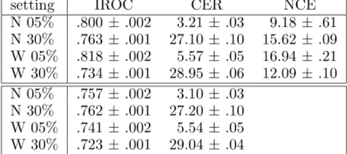
Table 2 shows the performance of the best configurations for classification and regression. The number of hidden units for each model is omitted because it has no clear correlation with performance. However, there is a clear trend in which classification models do better
setting IROC CER NCE
N 05% .800 ± .002 3.21 ± .03 9.18 ± .61 N 30% .763 ± .001 27.10 ± .10 15.62 ± .09 W 05% .818 ± .002 5.57 ± .05 16.94 ± .21 W 30% .734 ± .001 28.95 ± .06 12.09 ± .10 N 05% .757 ± .002 3.10 ± .03 N 30% .762 ± .001 27.20 ± .10 W 05% .741 ± .002 5.54 ± .05 W 30% .723 ± .001 29.04 ± .04
Table 2: Best results for classification (top box) and regression, with 95% confidence bounds. N and W stand for NIST and WERg in the problem setting column. Baseline values for CER are 3.21%, 32.5%, 5.65%, and 32.5% for each problem setting, in order. Note that the results on each line in this table are not necessarily generated by a single model.
than regression models, particularly as mea-sured by IROC. (This is not completely surpris-ing, given that classification MLPs were specifi-cally trained for the corresponding thresholds.) Globally, performance is better than the base-line in all cases except CER for the NIST 5% setting.
4.3 Feature Comparison
We compared the contributions of all features, both as individual confidence scores and as part of feature groups used to train MLPs. To group features, we classified them in two indepen-dent ways according to whether they apply to the source sentence, the target hypothesis, or both; and according to whether they depend on the base model or could be calculated with-out knowledge of it. We also treated the base-model’s scores as group on their own. All fea-ture experiments were performed only for the NIST 30% setting.
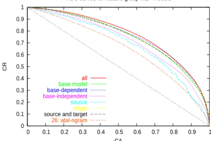
Results are shown in table 3 and figure 1. The most striking observation is that the MLP trained on only the twelve feature functions from the base model is almost as good as the one trained on all features. Another pattern is that features that depend on the base model are more useful that those that do not, and fea-tures that apply to the target hypothesis are more useful than ones that apply only to the source sentence (as well as, to a much lesser ex-tent, those that apply to a source/target pair). A final conclusion is that a model that has been trained on labelled data—regardless of the fea-ture set used—is better at discriminating than any single feature on its own.
0 0.1 0.2 0.3 0.4 0.5 0.6 0.7 0.8 0.9 1 0 0.1 0.2 0.3 0.4 0.5 0.6 0.7 0.8 0.9 1 CR CA
ROC curves for feature-group MLP models
all base model base-dependent base-independent source target source and target 26: atal-ngram
Figure 1: ROC curves for models trained on dif-ferent feature groups. Note that the “wiggly” ap-pearance of the curve for the source group is due to the fact that these features are invariant over all entries in a given nbest list, which leads the model to assign large blocks of examples exactly the same probability of correctness.
G IROC CER NCE
All .763 ± .001 27.10 ± .10 15.62 ± .09 Base .746 ± .001 27.82 ± .09 13.97 ± .08 BD .754 ± .001 28.02 ± .10 14.83 ± .10 BI .712 ± .001 29.88 ± .09 9.76 ± .09 S .687 ± .002 3.41 ± .07 7.23 ± .08 T .751 ± .001 27.91 ± .08 14.48 ± .09 ST .746 ± .001 28.47 ± .10 13.62 ± .07 S1 .648 ± .001 32.14 ± .08
Table 3: Results for models trained on different feature groups. All is all features, Base is base model scores; BD and BI are base-model dependent and independent; S, T, and ST are source, target, and both; and S1 is the best single feature.
5 Word-Level Experiments
It is not intuitively clear how to classify words in MT output as correct or incorrect when compar-ing the translation to one or several references. We implemented a number of different measures that were inspired by automatic evaluation met-rics like WER and PER.
Pos: This error measure considers a word as correct if it occurs in exactly this target position in the reference translation. WER: A word is counted as correct if it is
Levenshtein-aligned to itself in the refer-ence.
PER: A word is tagged as correct if it occurs in the reference translation. The word order is completely disregarded, but the number of occurrences is taken into account.
For all error metrics, we determine the refer-ence with minimum distance to the hypothesis according to the metric under consideration and classify the words as correct or incorrect with respect to this reference.
These error metrics behave significantly dif-ferent with regard to the percentage of words that are labeled as correct. Pos is very pes-simistic with only 15% correct words on the cor-pora described in section 3.1, whereas WER la-bels 43% as correct, and PER 64%, respectively. Note that those figures are not the translation errors for the system output. They are cal-culated for every hypothesis in the N -best list (and not only for the single best translation). 5.1 Features
We used 17 features in total which we will de-scribe shortly in this section. For more details, see (Blatz et al., 2003).
SMT Model Based Features
We investigated two features that are based di-rectly on namely the Alignment Template MT model (Och and Ney, 2004). One gives the iden-tity of the so-called Alignment Template, i.e. the bilingual phrase, that was applied in the translation of the current target word. Another feature specifies whether the target word was translated by a rule based system or not. This rule based system was integrated into the trans-lation process for the transtrans-lation of special phe-nomena such as dates and time expressions. IBM Model 1
We implemented one feature that determines the average translation probability of the target word e over the source sentence words according to Model1 introduced by IBM in (Brown et al., 1993). This captures a sort of topic or semantic coherence in translations.
Word Posterior Probabilities and Related Measures
We investigated three different features intro-duced in (Ueffing et al., 2003) that are calcu-lated rather similarly: relative frequencies, rank weighted frequencies and word posterior proba-bilities. Each of them is based on determining those sentences in the N -best list that contain the word e under consideration in a certain po-sition. The first variant (called any in table 4) regards all those sentences that contain e at all, whereas the second variant (source) considers all sentences where e occurs as the translation of the same source word(s). The third variant
(target) determines only those target sentences containing e in exactly the same position. Target Language Based Features
We implemented three different features using the semantic data provided by WordNet. The first similarity feature is the average semantic similarity from the word in question to the word aligned to the same source position in each of the top three hypotheses. The two other fea-tures come from WordNet’s polysemy count, for details see (Blatz et al., 2003).
Two more target language based features were implemented. One is a basic syntax check that looks to highlight hypotheses with mis-matched parentheses and/or quotation marks. The second feature counts the number of oc-curences in the sentence for each word in the target sentence.
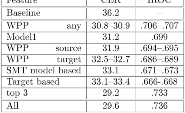
5.2 Performance of Single Features Using the Naive Bayes classifier, we tested the performance of single features for word confi-dence estimation. Additionally, we combined the best 3 and all 17 features with the same clas-sifier. Table 4 shows the confidence estimation performance of single features in terms of CER and IROC using the error measure PER for la-beling words as correct or incorrect. The fea-tures which yield the best results are the word posterior probability, rank weighted frequency, and relative frequency (WPP) with respect to occurrence of the word in any position in the target sentence. Those three features give a sig-nificant improvement over the baseline of more than 5% absolute in CER. The feature based on Model1 also discriminates very well, followed closely by the WPP with regard to the aligned source position(s).
The combination of three of the best performing features (word posterior probabilities with re-spect to different criteria and the Model1 based feature) yields a significant improvement over the performance of any of the single features. There is no significant change in CER or IROC if more information is added by combining all 17 features.
5.3 Comparison of Different Models For word level confidence estimation, we investi-gated several different MLP architectures, with the number of hidden units ranging from 0 to 20. Figure 2 compares the tagging performance for different MLP architectures and for the Naive Bayes classifier, including all features.
Feature CER IROC Baseline 36.2 – WPP any 30.8–30.9 .706–.707 Model1 31.2 .699 WPP source 31.9 .694–.695 WPP target 32.5–32.7 .686–.689 SMT model based 33.1 .671–.673 Target based 33.1–33.4 .666-.668 top 3 29.2 .733 All 29.6 .736
Table 4: CER [%] and IROC for single features and their combination using Naive Bayes; Word Error Measure: PER. 0 0.1 0.2 0.3 0.4 0.5 0.6 0.7 0.8 0.9 1 0 0.1 0.2 0.3 0.4 0.5 0.6 0.7 0.8 0.9 1 correct rejection [%] correct acceptance [%] NB MLP0 MLP5 MLP10 MLP20
Figure 2: ROC curves for PER, MLPs with differ-ent numbers of hidden units and Naive Bayes, com-bining all features.
We see that the Naive Bayes classifier and the MLP with zero hidden units have a very simi-lar performance. But as soon as the MLP gets more complex by the addition of more hidden units, the MLP outperforms the Naive Bayes approach significantly. There is no significant difference between the MLPs consisting of 5 to 20 hidden units.
5.4 Comparison of Word Error Measures
Table 5 compares the IROC values for word con-fidence estimation using an MLP with 20 hidden units for all the error measures described at the
Error Measure Pos WER PER IROC .734 .703 .766 Table 5: Comparison of IROC values of an MLP with 20 hidden units for different error measures (all features).
beginning of the section. We see that classifi-cation according to some of the error measures is easier to learn than according to others. The highest discriminability is obtained for the most “relaxed” measure PER, followed by Pos. As we had expected, WER is harder to learn, because the ratio of correct and incorrect words is almost equal.
6 Conclusion
We have reported on the use of various tech-niques for classifying MT output as correct or not, at both the sentence and word levels. Both levels present problems for the definition of cor-rectness. At the sentence level we resolved these problems by using automatic MT evalua-tion metrics and re-defining “correctness” to be above a certain threshold (of match to reference translations), which we feel should correspond to usability within different applications. At the word level we investigated three strategies, dif-fering in strictness, for matching corresponding words in reference translations.
Our main conclusions can be summarized as follows:
• Training a separate layer using machine-learning techniques is better than relying solely on base model scores.
• Features derived from the base model are more valuable than external ones, and should be tried first before investing effort in the implementation of complex external functions.
• Features based on nbest lists are more valu-able than ones based solely on individual hypotheses.
• Features that capture properties of the tar-get text are more valuable than those that do not.
• Multi-layer perceptrons (neural nets) out-perform naive Bayes models. MLPs with more hidden units can give better perfor-mance than those with fewer.
In future work, we look forward to using the techniques developed here within various appli-cations described in the introduction. We also intend to continue to refine our definitions of correctness to make them more stable and more broadly applicable.
Acknowledgement
This material is based upon work supported by the National Science Foundation under Grant No. 0121285.
References
C.M. Bishop. 1995. Neural Networks for Pattern Recognition. Oxford.
J. Blatz, E. Fitzgerald, G. Foster, S. Gandrabur, C. Goutte, A. Kulesza, A. Sanchis, and N. Ueffing. 2003. Confidence estimation for machine transla-tion. Final report, JHU / CLSP Summer Work-shop.
P.F. Brown, S.A. Della Pietra, V.J. Della Pietra, and R.L. Mercer. 1993. The mathematics of Ma-chine Translation: Parameter estimation. Com-putational Linguistics, 19(2):263–312.
R. Collobert, S. Bengio, and J. Mari´ethoz. 2002. Torch: a modular machine learning software li-brary. Technical Report IDIAP-RR 02-46, IDIAP. G. Doddington. 2002. Automatic evaluation of machine translation quality using n-gram co-occurrence statistics. In Proc. HLT-02.
R.O. Duda, P.E. Hart, and D.G. Stork. 2001. Pat-tern Classification. Wiley.
S. Gandrabur and G. Foster. 2003. Confidence esti-mation for text prediction. In Proc. CoNLL03. D. Guillevic, S. Gandrabur, and Y. Normandin.
2002. Robust semantic confidence scoring. In Proc. ICSLP’02.
C. Neti, S. Roukos, and E. Eide. 1997. Word-based confidence measures as a guide for stack search in speech recognition. In ICASSP’97.
G. Ngai and D. Yarowsky. 2000. Rule writing or annotation: Cost-efficient resource usage for base noun phrase chunking. In Proc. ACL’00.
NIST, editor. 2003. Proc. NIST Workshop on Ma-chine Translation Evaluation.
F.J. Och and H. Ney. 2004. The alignment tem-plate approach to statistical machine translation. Computational Linguistics. To appear.
A. Sanchis, A. Juan, and E. Vidal. 2003. Improv-ing utterance verification usImprov-ing a smoothed naive Bayes model. In ICASSP’03.
M. Siu and H. Gish. 1999. Evaluation of word con-fidence for speech recognition systems. Computer Speech and Language, 13(4).
N. Ueffing, K. Macherey, and H. Ney. 2003. Con-fidence measures for Statistical Machine Transla-tion. In Proc. MT Summit IX.
F. Wessel, R. Schl¨uter, K. Macherey, and H. Ney. 2001. Confidence measures for large vocabulary continuous speech recognition. IEEE Tr. Speech Audio Proc., 9(3).
R. Zhang and A. Rudnicky. 2001. Word level confi-dence annotation using combinations of features. In Eurospeech, pages 2105–2108.