How Income Contingent Loans could affect Return to Higher Education: a microsimulation of the French Case

HAL Id: hal-00369986

https://hal.archives-ouvertes.fr/hal-00369986

Preprint submitted on 23 Mar 2011

HAL is a multi-disciplinary open access

archive for the deposit and dissemination of sci-entific research documents, whether they are pub-lished or not. The documents may come from teaching and research institutions in France or abroad, or from public or private research centers.

L’archive ouverte pluridisciplinaire HAL, est destinée au dépôt et à la diffusion de documents scientifiques de niveau recherche, publiés ou non, émanant des établissements d’enseignement et de recherche français ou étrangers, des laboratoires publics ou privés.

How Income Contingent Loans could affect Return to

Higher Education: a microsimulation of the French Case

Pierre Courtioux

To cite this version:

Pierre Courtioux. How Income Contingent Loans could affect Return to Higher Education: a mi-crosimulation of the French Case. 2008. �hal-00369986�

How Income Contingent Loans could affect Return to Higher

Education: a microsimulation of the French Case

Pierre Courtioux (EDHEC Business School)

Abstract

The paper assesses the implementation of income contingent loan schemes for higher education (ICL) in an institutional context characterized by two main features: (i) a former tuition free system and (ii) a great heterogeneity in tertiary education’s diplomas quality and cost, which impacts the individual career paths. In this particular case, IC L implementation leads to a trade-off between increasing ‘career’ equity in terms of collective public spending versus individual gains and widening low education traps by reducing the economic incentives to pursue a tertiary education curriculum. Based on a dynamic microsimulation model we propose an ex ante evaluation of the enlargement of low education traps induced by the implementation of different ICL designs in France. We conclude that the risk of low education traps’ enlargement remains very small.

1. Introduction

The Income Contingent Loans (ICL) schemes have been implemented in some countries -noteworthy Australia and New-Zealand- mainly to develop higher education financial resources and to downsize credit shortage for low income families’ students. In an ICL financing scheme, tuition fees must be paid, but students can borrow from the State. Collecting the debt depends on the borrower capacity to pay back over her life course: above a certain income threshold, the borrower is supposed to pay back each year a fixed part of her income until her loan is recovered.

Financing higher education by ICL has been thoroughly discussed in education economics – for a review, see Chapman (2006a). Insofar as individuals finance their own higher education, ICL can be associated to a reduction in higher education subsid ies and the correspond ing tax burden; it then reduces the income regressivity of a no-charge education system; it can also diminish the problems generated by credit market failures; at last it can play a role in favour of the promotion of some career choices that are not well paid but socially desirable. Evidences on the practical consequences of implementing ICL are also documented in some

countries with different institutional designs and higher education problems they face – Chapman and Ryan (2003), Chapman (2006a). This paper assesses the question of ICL implementation in a particular case: the case of countries with (1) existing tuition- free system and (2) great heterogeneity in tertiary education’s diplomas’ quality and cost, which impacts the individuals’ career paths. We discuss the ICL implementation in this case with an ex ante evaluation for France, based on a dynamic microsimulation model.

Implementing ICL may have various consequences. First, implemented in a tuition- free system, it implies a reduction in the returns and a reduction in the gap between the individual gains and the collective cost of a degree. We focus on this aspect when we refer to the problem of equity. Second, the reduction in return may affect the individual decision to engage in tertiary education and the choice of the diploma. We do not assess directly this question; however we analyse the implication of ICL implementation on the distribution of expected gains. We focus on this aspect when we refer to the potential widening of low education trap.

The second section identifies the particular issue we asses in regard to the previous literature on ICL. We discuss the idea that in our particular case, implementing ICL leads to a trade-off between equity and the returns to higher education. Insofar as high enrolment rates in higher education are linked to the tuition- free system, increasing tuition costs to a level closer to the real education costs could lead to incentive problems. In some countries - like Australia– implementing ICL did not affect enrolment rates in tertiary education. However in countries with great heterogeneity in higher education costs for similar degrees –like France- the incentives for higher education enrolment could be substantially changed by introducing an ICL scheme, then potentially widening low education traps. In the third section, we discuss the way a dynamic microsimulation model tackling with the heterogeneity of life course considering diploma could assess this problem. Following this methodology, one can produce an ex ante evaluation of the impact of implementing an ICL schemes on the internal rate of return to higher education. We present a dynamic microsimulation model which illustrates the main features of the French case: especially career diversity considering diploma and the transfers’ system. In a fo urth section, we present the results of the simulation for different ICL schemes and their potential impact on internal rates of return. We then discuss the risk of enlarging low education traps in implementing ICL.

In this section, we identify key concepts to evaluate ICL implementation in France.We discuss the risk of enlarging low education traps when implementing an ICL system consistent with higher education’s real costs in a formerly tuition-free tertiary education system. Enlargement of low education traps could then be defined as the individual choice of not completing tertiary education because of changes in the money incentives to enter higher education.

In a first sub-section, we review the equity problem of ICL implementation and focus on what we identify as the career equity issue. We argue that the quantification of the trade-off between equity and low education traps remains a crucial problem which is context related. In a second sub-section, we point out the France as a polar case characterized by a concentration of higher education subsidies and a related differentiation of individual career. In this country, considering the actual higher education framework, implementing a higher education financing arrangement with a higher level of equity could lead to reduced returns to higher education.

2.1. Income Contingent Loan implementation: learning from international comparisons There are several motivations to implement ICL scheme for higher education: (i) generalize a financial arrangement less costly than scholarship, (ii) increase enrolment rate of students with poor family background, (iii) enable individuals to access not well paid careers which however produce wide positive externality, (iv) increase resources for higher education, (v) implement a financial arrangement more progressive with income –see Chapman (2006b) for a review. The relative importance of these motivations differ according to countries and the problems their educational system faces. For instance the need of resources for higher education, the will to downsize the importance of default protection in the repayment of a loan, and the will to decrease the regressivity of a no-charge system seem important objectives considered for the launching of ICL schemes in Australia and New Zealand. In the United States, it is the problem of conventional loan repayments and their implication for career choices which seems to have been central in the decision of implementing an ICL scheme -Chapman (2006a). In our particular case –e.g. tuition-free higher educational system with a great heterogeneity in tertiary education’s diplomas real cost –the scope of the benefits of an ICL implementation need to be precisely defined.

In a first hand, the ICL scheme could increase resources for higher education. Insofar as higher educational costs are already subsidized –e.g. financed by taxes-, the increase in resources is linked to the collection of the debt over the life course. This means that the

increase in resources available is a long term objective of the ICL implementation. Moreover, without a reform of the financial arrangements between Universities and State, implementing an ICL scheme collected by tax administration has no direct effect on Universities financial resources. We do not focus on this particular point.

In a second hand, the ICL scheme could increase equity. From an income analysis point of view, a tuition free higher education system is regressive insofar as higher education enrolment is linked to family income. This first income-regressive effect could be called the ‘family’ effect. It was expected to be small in a tuition-free higher education system –the actual income-regressive ‘family’ effect could remain in a no charge system, as suggested by the Australian debates in the 80’s (Chapman, 2006b). This first income-regressive ‘family’ effect is reinforced by an income-regressive ‘career’ effect for higher educated workers due to the wage premium attached to their diploma. If the differential wage premium of the different diploma s is linked to the real teaching costs, an ICL scheme which charges the students according to their real teaching costs is supposed to reduce the ‘career’ income-regressive effect of higher education.

Considering the particular case of a no-charge higher education system with a great heterogeneity in tertiary education costs, the main goal of implementing an ICL scheme could be to reduce the ‘career’ income regressive effect.

However, a main drawback of implementing ICL in a tuition-free system is that it reduces return to higher education. The students enrolled in higher education have to pay back their education costs –or a part of it- over their life course. This change increases equity. Indeed, in the former system, the training cost was entirely paid by the State, whereas the diploma benefits are mainly captured by the forme r student –nevertheless a part of this wage premium is paid back to the State by means of progressive taxes and some benefits can be collective through externalities. In the new situation the diploma cost is paid by the State and the former student. Implementing ICL scheme could then produce low education traps if the net wage premium for higher education is substantially reduced. The incentive to complete a higher education degree is downsized. With imperfect information, this effect could counter-balance the effect of increasing ‘career’ equity in so far as the risk of having high educated poor careers could only be supported by students from higher income families. Low education traps could then be defined as a global incentives’ scheme which favours the choice of not pursuing tertiary education.

Few evaluations which assess the problem of low education traps for poor background individuals linked to ICL implementation are available. They concern mainly the Australian

and the New Zealand cases which are generally considered as successes. The New Zealand case is the most far away from the case we assess in this paper, because ICL scheme was implemented in a higher education system with already existing fees for higher education. However, the available evaluations point out some interesting results reported in Chapman (2006a). For instance, Maani and Warner (2000) note a decrease in Maoris’ enrolment in higher education following the ICL implementation –historically in this country the Maoris constitute an ethnic group with relatively poor background. However, LaRocque (2005) considering the period after the 2000’s reform which tends to introduce more income progressive measures in the ICL scheme finds an increase in the Maoris’ enrolment.

The Australian experience is closer to the case we assess insofar as ICL schemes were implemented in a tuition- free higher education system. The available evaluation tend s to show that there is no effect on poor background individuals enrolment rate in higher education: Andrew (1999), Long et al. (1999), Marks et al. (2000), Chapman and Ryan (2002) found no evidence in this perspective, whereas Aungles et al. (2002) notes a decrease in poor background individuals enrolment rate after 1996 ICL’s reform, but the robustness of the result is questioned –see Chapman (2006a) for a comment.

When one considers implemented ICL policies, there is a tendency to link real higher education cost and ICL schemes, but it remains relatively underdeveloped. For instance, in Australia, the Higher Education Contribution Scheme (HECS) changes of 1996 could be interpreted as a reform in this way. The HECS is an ICL scheme that was launched in 1989 with a uniform charge whatever is the subject area of the student. The 1996’s reform introduces thr ee differentiated charge s by broad subject area. According to Chapman (1998), this differential charge reform transformed the Australian higher education system into a hybrid model: this new arrangement goes further in closing the gap between fees and costs, but it is not actually consistent with a pure cost recovery model. Moreover, from a European point of view, considering the Lisbon Strategy and its related guidelines for education, introducing higher fees for scientific diploma seems not consistent with the so-called ‘Education and Training 2010’ guidelines: one of the main goal is to increase recruitment in scientific and technical studies –see for instance Commission of the European Communities (2005).

From a more general point a view, ICL is a tool to develop ‘career’ equity; it reduces the gap between individual costs and individual return to education over the life course. In this regard, the few existing experiments are not ‘purely’ transferable, because one needs to identify the degree of polarization of higher education subsidies in the national system, as well as the

distribution of career under a given national socio- fiscal regime. The question of how far national policy can go in reducing income-regressive ‘career’ effect of higher education without creating low education traps remains a crucial problem in the discussion of ICL implementation, and more generally in promoting the ICL principle. This question is context related.

2.2. Equity and the diversity in Higher Education Cost: The French Case

Considering the question of developing ‘career’ equity with ICL in a higher education tuition-free system, France is interesting when one considers the great heterogeneity of tertiary education’s paths and of their corresponding costs. This heterogene ity goes beyond the evidence that scientific diplomas are generally more costly than other diplomas, and relates to the different institutions in charge of higher education paths and their place in the educational system.

Traditionally, at the end of High School, students have to choose between two paths: the State Universities and the Higher Education’s Schools (Grandes écoles). The Universities education path is a quasi no-charge system whatever the subject area chosen by the student. The higher educatio n’s School path is a two steps path. The first step consists of two years in a Preparatory class to higher education Schools (Classe préparatoire aux grandes écoles) which is subsidized by the State and free from charges. The second step is a three years’ step in a Higher Education School. For this second step the choice of the student subject area has financial consequences: Engineering Schools are subsidized by the State, whereas Business Schools are not largely subsidized and charge their students with high fees. Aside these two traditional main paths, there is some other specific diplomas: the Higher Technician Certificated (Brevet de Technician du Supérieur) diploma is prepared in two years in specific schools, whereas the University Institute of Techno logy Diploma (Diplôme Universitaire de

Technologie) and the Scientific and Technological University Diploma (Diplôme d’Etude Universitaire Scientifique et Technique) are two years specialized diplomas prepared in some

Universities.

The amount of public spending for a student is thus in France strongly related to her higher education path. These differences stem mainly from staff spending: Preparatory Classes and higher education Schools are mainly based on small classes’ pedagogy, whereas University’s courses are mainly done in amphitheatres.

Few statistics are available on diploma’s real cost in France. The table 1 gives an idea of the different costs of higher education paths corresponding to the part of the cost subsidized by

the State. The costs presented in this table are an evaluation based on the Zuber (2004) results, with some additional hypotheses concerning University cost for a year. We assume that all students follow the cheapest courses, for instance Law and Economics courses for a two years university degree. Following the Zuber (2004) results, we cannot present differentiated costs between the University diplomas; however these costs are probably higher for the University Institute of Technology Diploma (DUT) and the Scientific and Technological University Diploma (DEUST) than those of the regular University first degree (DEUG).

Table 1. Subsidized Higher Education Costs according to Education Path

Part of the 1970's generation

Public Higher Education Costs in € (2005)

No Higher Education Diploma 67.8% 0

Two years graduates 15.4% 13,298

DEUG (University) 1.5% 4,905

DUT/DEUST (University) 2.0% 4,905

BTS 8.9% 18,491

Other Higher Technician Diploma 0.6% 18,491

Paramedical Diploma 2.3% 4,764

Three years graduates 5.6% 14,072

Licence (University) 3.9% 8,486

Others three year graduates 1.6% 27,737

Four years graduates 3.9% 12,066

Master (University) 3.9% 12,066

Five years graduates 6.0% 32,709

DEA (University) 1.2% 17,805

DESS (University) 1.9% 17,805

Business Schools 0.9% 25,391

Engineering Schools 1.6% 58,838

Most 'prestigious' Engineering Schools 0.4% 127,527

More than five years graduates 1.4% 75,768

PhD (Medical Degree excluded) 0.7% 35,021

PhD (Medical Degree) 0.7% 113,892

Total 100% 6,288

Source: Zuber (2004), French Labour Force Survey 1990-2005 (Insee) – author’s calculation.

Differences in individual higher education costs stem from the number of years of education, the education path and the major.The cost of an additional year of higher education differs greatly according to the education path. The average cost per year for a two years University diploma is 2,453 euros, whereas the average cost per year for an Engineering School diploma

is near five times higher. When we consider also the years in Preparatory schools, the total cost of an Engineering School diploma is twelve times larger. This difference is only partially explained by the increasing cost of a year of higher education with the level of education. When one considers the same level of education, Engineering School costs are more than three times higher than the same level University degree. When one considers the most ‘prestigious’ Engineering School which represent around 1.9% of the total engineer degrees, the subsidized cost is more than sixteen time higher than a five years’ University degree. One can argue that these cost differences could be explained by the fact that scientific courses which constitute the main part of Engineering School curriculum are more costly. As shown in the previous section, implementing an ICL with a difference in tuition fees by major is not consistent with the Lisbon Strategy. However, according to Zuber (2004) evaluations, the differences in costs still remain. If one only considers the scientific major at University, Engineering Schools remain one and a half more costly. Moreover the cost gap between the most famous Engineering Schools and the other five years degree remains.

To conclude, French higher education system is characterized by education paths which differ by their selectivity and the costs paid by the State. Insofar as this higher education impacts individual careers, charging the diploma according to their collective cost could introduce more equity. Considering the implementation of an ICL scheme consistent with the Lisbon Strategy, the great diversity of degree cost goes beyond the traditional differences between scientific and other major fields of education. In France, this is mainly due to the diversity of higher education paths.

3. Analysing Higher Education Output over the Life course with a dynamic

microsimulation model

According to the traditional approach in education economics, education can be considered as a part of human capital which impacts earnings over the life course. The gains of this investment can be assessed by computing the individual internal rate of return of one additional year of education. Since the seminal Mincer (1974), measuring internal rate of return to education has become an important dimension of the analysis of education choices, which put the stress on controlling endogeneity -Heckman et al (2006). A complementary approach, still under developed in education economics, is the dynamic microsimulation method which aims at taking into account the complexity of national socio- fiscal regimes – for instance, Harding (1993), Mitton et al. (2000). These methods lead to the computation and

the analysis of ex post internal rate of return to education. They simulate the diversity of career in a given tax and transfer regime: basically, the micro- units are considered one year older each new step of the simulation. This ageing process affects the probability of changing labour market position, wages and the corresponding taxes and transfers. Considering education economics, the advantage of a dynamic microsimulation approach is to include in the calculation of the internal rate of education the whole tax and benefit system: for instance, a more complete calculation of education internal rate can be produced if pension schemes and more generally the last part of the life course are taken into account. As other empirical micro approaches, microsimulation enables an analysis of the distribution of individual internal rates of return to education for a given diploma.

To evaluate the distribution of internal rate of return to higher education, we have to produce individual chronicles of income s and taxes based on diploma characteristics. Harding (1995) analyses the ICL implementation in Australia on the basis of a ‘general’ dynamic microsimulation model which produces no specific results concerning education output. Her main focus is the forecast of the percentage of individuals who will pay back their loan and the differences between male and female considering this point. Vandenberghe and Debande (2007) produce a comparative microsimulation analysis of ICL schemes implementation for three countries –Belgium, Germany and United-Kingdom- ; however, they also retained a very aggregated variable for higher education diplomas. As shown in the previous section, when one considers higher education costs, this level of aggregation is not sufficient to assess particular cases like France.

A dynamic microsimulation model can be defined by the data it uses and the integrated ageing process.

We simulate the life course of 34,643 individuals who represent the ind ividuals born in 1970 –around 850,000 persons- in terms of sex, diploma and entering labour force’s ages. The relative percentage of each case is approximated on the basis of the French Labour Force Survey (FLFS) 2003-2005 considering the persons born in the 1968-1972 period. Actually, the real cost of teaching differs greatly between Engineering schools according to their ‘prestige’ e.g. their rank in the French higher education system - for more details see Zuber (2004). We decided to take into account this differentiation between Engineering Schools. Because classification in the French Labour Force Survey 2003-2005 (FLFS) doesn’t allow the statistician to distinguish those who got their degree from a Prestigious Engineering School from the others, we proceed to a partic ular methodology explained in section 6.5 in order to estimate wage equations.

The modelled ageing process simulates the annual individual transitions between three main states: inactivity, employment and unemployment –for more details see section 6.2. The simulation begins at sixteen which is the legal age for the end of compulsory schooling. A Mincer’s equation estimated by diploma is used to simulate the wage for individuals in employment position. The equations corresponding to the transition process and the wages simulation are estimated on the FLFS 2003-2005. Then we simulate the main features of the French socio-fiscal regime: unemployment benefits, retirement pensions and income tax –See section 6 for more details. The probability to survive is calculated until the individual is 100 – we then assume that she dies.

To calculate the internal rate of return at sixteen (r ), we need all the financial flows linked to _i

an investment: the internal rate of return is the rate of actualisation which makes the sum of these financial flows equal to zero. This condition can be written as follows:

0 ) 1 ( 84 1 = + − = =

∑

Where F is the net financial flow at age (a+15).The microsimulation approach enables us to _ia

apprehend the financial flows by diplomas all over the life course. These flows are growth earnings, which mix gains from all education years including primary and secondary schooling. To have an appraisal of the net impact of higher education, we decided to assume that the net financial flows linked to higher education is the difference between the individual net income and the expected income for the persons without tertiary diploma of the same age.

a ia ia ia ia ia ia W D R T O Gd F =( + + − )− − 0

Where W is the individual wage at the age (a+15), D the unemployment benefit, R the ia

retirement benefit and T the individual tax (individual income tax and ICL annuity), G 0d _a is

the income flow mean at the age (a+15) of the individuals who do not have a higher education degree. The opportunity (O_dxai) costs of an individual i, with a dx diploma level are calculated

as follows:

}

{

dxai MAX GLF GLF GLF

0 =

dxai

O if ALF_i >a

Where ALF is the age of entering the labour force of an individual i, and i GLFdxa the mean

of the gains at age (a+15) of the individuals with the dx higher education level who are in the labour force.

Two limits of dynamic microsimulation are generally admitted: (i) the dynamic of ageing is sensitive to assumptions –or implicit assumptions- about the macro conditions; (ii) without the modelling of behavioural response, the ex ante analysis of a programme imple mentation remains a ‘morning after’ analysis and could then be misleading if implementing such a programme implies behaviour modification. Considering the first point, the implicit assumption of our model is that the situation of the 2003-2005 reflects the wage s and the transitions perspectives as well as their heterogeneity for the 1970’s generation. The results we produce could be misleading if for instance there was a technological shock which should modify relative transition probabilities or wages during the period we simulate. Considering the second point, the model describes forecast of career heterogeneity without behaviour adjustment to the policy implementation. In this sense, it is a comprehensive simulation of internal rate for higher education diversity.

From a rational choice point of view, the evaluation of the impact of ICL implementation on the expected internal rate of return to higher education could be interpreted as measuring the potential change in incentives to comp lete a higher education degree: the expectation of internal rate of return and its variability, as well as her own qualities and aptitudes to learn are parts of the information set used by the student to determine her Higher educational strategy. If, for a given diploma, an important part of individual expected rate of return to higher education became negative or null with the implementation of ICL schemes, this could be interpreted as a potential enlargement of a low education traps.

4. An evaluation of ICL implementation

This section presents the results of our simulation of different ICL schemes. It appears that in spite of differentiated potential impact on macro level, the ICL schemes retained here have small impact on rate of return to higher education diploma; moreover they do not change the diplomas hierarchy. In the first subsection we focus on the design of the different schemes we simulate and their different macro impact. In the second one, we present the result considering the distribution of the diplomas’ rate of return.

4-1-The differences in the ICL schemes design and their macro impact

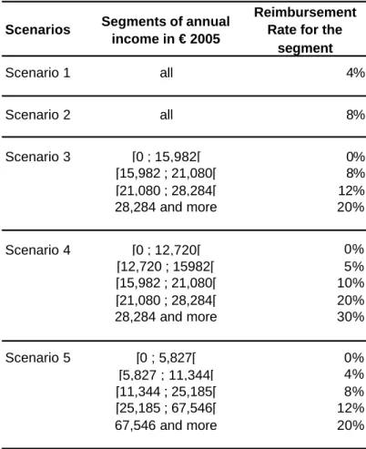
To measure how ICL could affect return to higher education, we simulate five different schemes that we compare to the reference which is the estimation of return to higher education in the present French case. The designs of the different schemes simulated are synthesized in table 2.

Table 2. The ICL schemes simulated

Scenarios Segments of annual income in € 2005

Reimbursement Rate for the

segment Scenario 1 all 4% Scenario 2 all 8% Scenario 3 [0 ; 15,982[ 0% [15,982 ; 21,080[ 8% [21,080 ; 28,284[ 12% 28,284 and more 20% Scenario 4 [0 ; 12,720[ 0% [12,720 ; 15982[ 5% [15,982 ; 21,080[ 10% [21,080 ; 28,284[ 20% 28,284 and more 30% Scenario 5 [0 ; 5,827[ 0% [5,827 ; 11,344[ 4% [11,344 ; 25,185[ 8% [25,185 ; 67,546[ 12% 67,546 and more 20%

In the two first schemes, we assume that the annual reimbursement is a fixed amount of the current income respectively 4% and 8%, whatever is the level of income. Insofar as there is no threshold of exemption to reimbursements, they do not correspond to the very ICL principle. These two scenarios are benchmarks, notably to evaluate the macro aspects of reimbursement. The scenario 3 and the scenario 4 have a design corresponding to the percentiles of hourly wages normalised on an annual basis. The reimbursement threshold of the scenario 3 is given by the median; the other thresholds of the other segments are respectively given by the third quartile and the 90th percentile. The reimbursement threshold of the scenario 4 is fixed on the first quartile; the thresholds of the others income segments are respectively given by the median, the third quartile and the 90th percentile. The last simulation is more embedded in the French tax system. The reimbursement thresholds correspond to the different thresholds of the French income tax. Technically the threshold of ICL’s reimbursement is largely below the fifth percentile of hourly wage. This means that the individuals who do not pay back ICL annuity are those who stay out the labour force or those who are without current income because of a long unemployment period. Comparing to the benchmarks the reimbursement rates are lower for the lower segments of income.

It is important to note that the different reimburseme nt schemes considered here differ significantly from the ones experimented in Australia. In Australia, when the current income is above the reimbursement threshold, the former student has to pay back a fixed part of her whole current income, whereas in the schemes we evaluate the rate of reimbursement is applied to the corresponding segment of the current income.

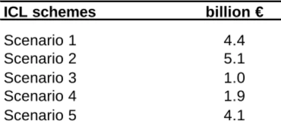
Of course, the different ICL schemes impacts on individuals have to be related to the financial resources they produce for the State. As noted earlier, the financial resources corresponding to a fully developed ICL scheme is only a long term goal. However, it has to be noticed that this amount varies according to the selected ICL scheme –see table 3.

Table 3. The different ICL schemes revenues (in 2005 €)

ICL schemes billion €

Scenario 1 4.4

Scenario 2 5.1

Scenario 3 1.0

Scenario 4 1.9

Scenario 5 4.1

Source: author’s calculations.

Note: to calculate the ICL schemes aggregate amount, we assume that the total population is composed of overlapping generations with the characteristics of the 1970’s one; the whole simulation of the 1970’s generation life course is then considered as cross -section data.

Scenario 1 and scenario 2 are not income progressive, but only income proportional: fully developed, they lead to a flow between four and five billions euros. The amount is very sensitive to the reimbursement threshold. Scenario 3 fixes it at the level of the median hourly wage and scenario 4 at the level of the first quartile of hourly wage ; this leads to a decrease of more than half of the outcomes compared to the benchmarks. The last scenario whic h is an income progressive version of the two first scenarios with a very low reimbursement threshold have a total amount more close to the benchmarks.

Considering respectively the GDP of France and Australia and the Australian HECS revenue in 2004-2005 which are available in Chapman (2006b, p.81), one can argue that the ICL of the fourth scenario provide comparable revenues to the Australian situation. However, beyond these macro considerations, it is important to consider the individual level and the impact of such scheme on internal rate of return to higher education.

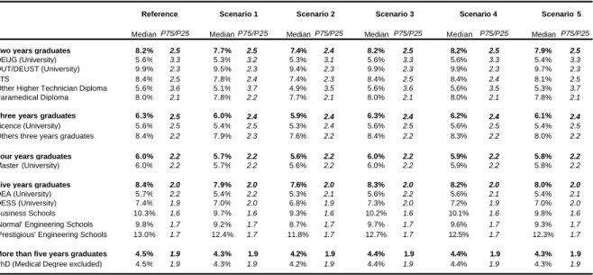
4-2-The impact on the distribution of individual rates of return to higher education Table 4 presents the results of the simulations considering the internal rate of return to higher education. A first set of comments concerns the actual return to higher education in France. The level of return does not increase with the years of higher education completed. The two years graduates have a relatively high median rate (8.2%); the median rate decreases sharply for the three years (6.3%) and slightly for the four years graduate (6%). The five years graduates have rate which is close to the two years graduates whereas there is an important decrease median rate for the PhD (4.5%). This quite surprising result is explained by the heterogeneity of higher education paths exposed in section 2.2. When one considers for instance the regular University curriculum, the returns to higher education are not so

surprising: if the DEUG rate is close to the Licence rate, it is significantly lower than the Master rate. This trend pursues for the more applied University degree –the so called ‘DESS’- but it decreases for the more general University Degree –the so called ‘DEA’.

More generally, the results concerning the completed five years or more diplomas have to be interpreted carefully: the relative low rates of return to University diploma s is linked to their relatively small part in the high wage sectors, where they compete with engineers. Similarly, the relative ly low rate of return to other PhD diplomas could be explained by the relatively small part of scientific and technical majors, which remains Engineering School’s speciality in French higher education system. This trend is certainly reinforced by specific career choice of PhD graduates, notably in the education sector, which are not well paid considering the level of education completed for PhD diplomas. Moreover, the PhDs’ tend to enter lately in the labour force; it mechanically impacts negatively the rate of return for an equivalent first wage. Concerning the medical PhD diplomas, we choose to not reproduce the results, because they are based on the estimation of wage equations whereas an important part of these persons engages in a self-employment career –see 6-3 for more details.

Not surprisingly, the diplomas with the highe st rates of return are those of the ‘most prestigious’ Engineering Schools (13%). They are followed by Business School degrees (10.3%). The other Engineering Schools degrees have a median rate of return equivalent to the rate of very specialized two years degree completed at University –the DUT and DEUST degrees- which do not correspond to the regular University education path: 9.8-9.9%. Some other very specialized two or three years degrees have also high rate of return to diploma (around 8%): BTS, three years graduates not completed at university and paramedical diploma.

Table 4. Return to Higher Education

Median P75/P25 Median P75/P25 Median P75/P25 Median P75/P25 Median P75/P25 Median P75/P25

Two years graduates 8.2% 2.5 7.7% 2.5 7.4% 2.4 8.2% 2.5 8.2% 2.5 7.9% 2.5

DEUG (University) 5.6% 3.3 5.3% 3.2 5.3% 3.1 5.6% 3.3 5.6% 3.3 5.4% 3.3

DUT/DEUST (University) 9.9% 2.3 9.5% 2.3 9.4% 2.3 9.9% 2.3 9.9% 2.3 9.7% 2.3

BTS 8.4% 2.5 7.8% 2.4 7.4% 2.3 8.4% 2.5 8.4% 2.4 8.1% 2.5

Other Higher Technician Diploma 5.6% 3.6 5.1% 3.7 4.9% 3.5 5.6% 3.6 5.6% 3.5 5.3% 3.7

Paramedical Diploma 8.0% 2.1 7.8% 2.2 7.7% 2.1 8.0% 2.1 8.0% 2.1 7.8% 2.1

Three years graduates 6.3% 2.5 6.0% 2.4 5.9% 2.4 6.3% 2.4 6.2% 2.4 6.1% 2.4

Licence (University) 5.6% 2.5 5.4% 2.5 5.3% 2.4 5.6% 2.5 5.6% 2.5 5.4% 2.5

Others three years graduates 8.4% 2.2 7.9% 2.3 7.6% 2.2 8.4% 2.2 8.3% 2.2 8.0% 2.2

Four years graduates 6.0% 2.2 5.7% 2.2 5.6% 2.2 6.0% 2.2 5.9% 2.2 5.8% 2.2

Master (University) 6.0% 2.2 5.7% 2.2 5.6% 2.2 6.0% 2.2 5.9% 2.2 5.8% 2.2

Five years graduates 8.4% 2.0 7.9% 2.0 7.6% 2.0 8.3% 2.0 8.2% 2.0 8.0% 2.0

DEA (University) 5.7% 2.2 5.4% 2.2 5.3% 2.1 5.6% 2.2 5.6% 2.1 5.4% 2.1

DESS (University) 7.4% 1.9 7.0% 2.0 6.8% 1.9 7.3% 2.0 7.2% 1.9 7.0% 2.0

Business Schools 10.3% 1.6 9.7% 1.6 9.3% 1.6 10.2% 1.6 10.1% 1.6 9.8% 1.6

'Normal' Engineering Schools 9.8% 1.7 9.2% 1.7 8.7% 1.7 9.7% 1.7 9.6% 1.7 9.3% 1.7

'Prestigious' Engineering Schools 13.0% 1.7 12.4% 1.7 11.8% 1.7 12.7% 1.7 12.5% 1.7 12.3% 1.7

More than five years graduates 4.5% 1.9 4.3% 1.9 4.2% 1.9 4.4% 1.9 4.4% 1.9 4.3% 1.9

PhD (Medical Degree excluded) 4.5% 1.9 4.3% 1.9 4.2% 1.9 4.4% 1.9 4.4% 1.9 4.3% 1.9

Scenario 4 Scenario 5 Reference Scenario 1 Scenario 2 Scenario 3

Source: author’s calculations.

Note: the simulation concerns the 1970’s generation.

A higher rate of return is not the only output that could explain enrolment in higher education. Higher diplomas are expected to secure careers which could be measured by distribution statistics like the distance between percentiles of rate of return to diploma – the P75/P25 columns of table 4. In this perspective, the heterogeneity of careers is reduced with the years of higher education completed. Generally when considering diplomas at the same level of education, the higher is the return the smaller is the distribution variance or interquartile range.

The ICL schemes which uniformly charge a fixed amount of the current income until the debt is recovered have a small impact on the median rate of return to higher education. For a charging rate of 8% of current income (scenario 2), the maximum decrease in rate of return to diploma is 1.2 point. It concerns the ‘most prestigious’ Engineering School. This kind of ICL schemes has quasi no impacts on rates of return distribution whatever is the level of education or the diploma: the maximum is an increase in P75/P25 of 0.2 point for the DEUG University degree.

When one considers the ICL schemes with income-progressive reimbursement rate (scenario 3, 4 and 5), the maximum decrease in the rate of return is 0.7 point. Like for other scenarios the maximum decrease concerns the ‘most prestigious’ Engineering Schools. Scenarios 1 and 2 which have a higher reimbursement threshold than the scenario 3, do not change the median rate of return for two years degree and slightly decrease the return for three and four years

degree. Like the uniformly charged ICL schemes the progressive ICL schemes has quasi no impact on rates of return’s distribution.

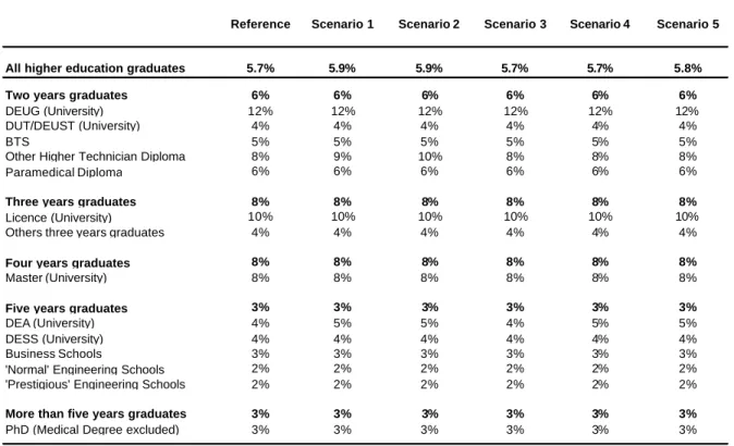
Noteworthy, the diplomas hierarchy remains unchanged whatever is the ICL scheme considered, which means that the relative financial incentives to complete a diploma will not be affected by the introduction of an ICL scheme. However, an ex ante evaluation of ICL implementation has to consider if it potentially increases low education traps. In this perspective, the table 5 presents the proportion of the individual rates of return to higher education which are negative; this means that the earnings of these persons with a tertiary education are inferior to the mean earnings of individuals who did not complete a higher education degree. From a rational point of view considering expecting gains -without considering the individual talents for education-, the decision to complete higher education for these level of degree has a very uncertain outcome.

Table 5. Proportion of Negative Individual Returns to Higher Education

Reference Scenario 1 Scenario 2 Scenario 3 Scenario 4 Scenario 5

All higher education graduates 5.7% 5.9% 5.9% 5.7% 5.7% 5.8%

Two years graduates 6% 6% 6% 6% 6% 6%

DEUG (University) 12% 12% 12% 12% 12% 12%

DUT/DEUST (University) 4% 4% 4% 4% 4% 4%

BTS 5% 5% 5% 5% 5% 5%

Other Higher Technician Diploma 8% 9% 10% 8% 8% 8%

Paramedical Diploma 6% 6% 6% 6% 6% 6%

Three years graduates 8% 8% 8% 8% 8% 8%

Licence (University) 10% 10% 10% 10% 10% 10%

Others three years graduates 4% 4% 4% 4% 4% 4%

Four years graduates 8% 8% 8% 8% 8% 8%

Master (University) 8% 8% 8% 8% 8% 8%

Five years graduates 3% 3% 3% 3% 3% 3%

DEA (University) 4% 5% 5% 4% 5% 5%

DESS (University) 4% 4% 4% 4% 4% 4%

Business Schools 3% 3% 3% 3% 3% 3%

'Normal' Engineering Schools 2% 2% 2% 2% 2% 2%

'Prestigious' Engineering Schools 2% 2% 2% 2% 2% 2%

More than five years graduates 3% 3% 3% 3% 3% 3%

PhD (Medical Degree excluded) 3% 3% 3% 3% 3% 3%

Source: author’s calculations.

Note: the simulation concerns the 1970’s generation.

A first range of comments concerns the part of individual negative return to higher education in the reference situation - e.g. without any ICL scheme implementation. Among the higher education graduates they are about 6%. There are two kinds of explanations for this situation. In a first hand, this negative rate could be related to career choices –entirely or partially

constrained by the institutional framework. For instance women could decide to complete higher education but will quit the labour force for child care; in doing so, their individual rate of return to higher education decreases, even if the welfare provided by this education choice is better than the choice of not completing a higher education degree. In a second hand, this situation could be explained by imperfect information on the hierarchy of diplomas expected returns and/or on student knowledge of its own ability to gain from a completed diploma on the labour market considering local conditions, etc.

Insofar as the education process is long, one expects that the part of negative return to higher education will decrease. Our results show (table 4) that it is not verified. The two years degrees which have a rate close to the mean, whereas there is an increase in this rate for the three and four years graduates. As for the median rate of return to diploma, this can be explained by diplomas heterogeneity. When one considers the regular University path –e.g. DEUG, Licence, Master, DEA/DESS and PhD-, the proportion decreases.

With a risk of 2-3%, Engineering Schools and Business Schools are associated with the smallest risk of negative return. The higher rates concern the two years graduates of the University regular education path which reaches 12%. More generally, the University regular education path’s diplomas have a relatively important part of negative returns until the master degree (8%). An explanation of this concentration of the risks of negative returns on the University path is that having a University diploma is a signal that the student has not been able to complete a higher degree following the regular University education path; this leads to a more important risk of junked career.

The impact of ICL schemes implementation on the part of negative returns to higher education remains small. According to the schemes considered, it increases the global part from 0.1 point to 0.2 point. However, when one considers specific diplomas, the risk increase could be a little more important –but always below one point. The more vulnerable diplomas are the University’s five years general degree –DEA- and the ‘Other Higher Technician’ Diplomas.

5. Conclusion

In this paper we analysed the question of implementing ICL schemes for higher education in the case of an institutional context characterized by a former tuition free system and a great heterogeneity in tertiary education diplomas quality and cost which impact the individual’s careers. We discuss the problem of equity in this context and argue that the principal

justification of ICL implementation is the development of ‘career’ equity, with a related risk: the creation of low education traps. Based on a microsimulation of the French case, which is characterized by a great heterogeneity of higher education diplomas, we show that this risk remains small whatever is the particular design of the ICL scheme imp lemented. Moreover a more income-progressive scheme leads to contain the progression of these low education traps measured by the part of negative individual rates of return to higher education. More generally, the tertiary education diplomas hierarchy is not affected by an ICL implementation. Concerning higher education policy, this paper shows that implementing ICL scheme could be extended to countries with complex and heterogeneous tertiary education system: it has a very small impact on return to higher education. This could lead to increase ‘career’ equity - in this view, our results complement those of Vandenberghe and Debande (2007) for a more extreme country case considering the heterogeneity of tertiary education’s costs. Moreover, the ICL implementation could lead to collect additional resources which could be invested in tertiary education. However, from a welfare point of view, complementary evaluations should be produced concerning the impact of the different ICL schemes on households’ disposable income over the life course to have a more complete evaluation of the implementation of this kind of schemes and the corresponding living standard risks.

6-

Annex: the microsimulation model

The microsimulation model aims at simulating the individual sources of income over the ir life course considering the diploma they completed. In this annex, we present the architecture and the different hypotheses of the dynamic microsimulation model which we use in the paper. In a first sub-section we present the main hypotheses that are made to simulate the aggregate labour force participation of a given generation over its life course. These results are used in the model for the statistical alignment of individual transitions. In a second sub-section we present the main hypotheses concerning the simulation of individual transitions. In a third sub-section, we present the main hypotheses concerning wage simulation. In a fourth one, we present the way we assess the case of the ‘most prestigious’ Engineering Schools. In the last sub-section, we shortly describe the main features of the French socio-fiscal regime, which are taken into account in the model.

6-1-Modelling generational labour force participation and unemployment rate over the life course

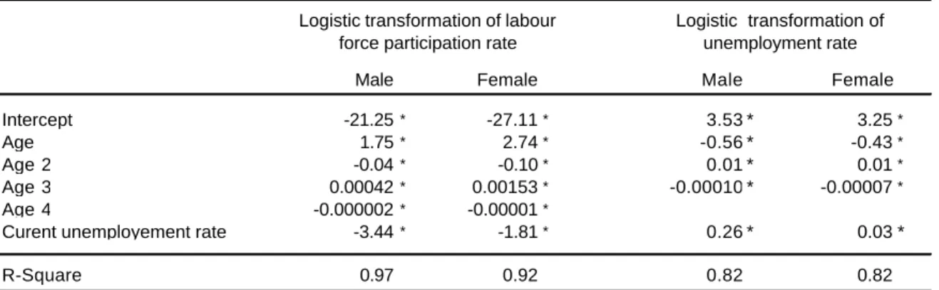
A first step consists of modelling the rate of labour force participation and the unemployment rate over the life course for a given generation. The French Labour Force Survey 1968-2005 is used to construct segments of labour participation rate and unemployment rate according to age and generation. For instance, the generation born in 1950 has available data from the age 18 to 55, the generation born in 1960 from the age 16 to 45, the generation born in 1970 from 16 to 35, etc. The model is estimated separately for males and females; it includes different specifications of age, the current unemployment rate for a generation at a given age and generations’ dummies. The main results of the estimations are presented in table 6.

Table 6. Estimation of Labour Force Participation and Unemployment Rate Models

Male Female Male Female Intercept -21.25* -27.11* 3.53 * 3.25*

Age 1.75* 2.74* -0.56 * -0.43*

Age 2 -0.04* -0.10* 0.01 * 0.01*

Age 3 0.00042* _0.00153* _{-0.00010 * -0.00007}*

Age 4 -0.000002* -0.00001*

Curent unemployement rate -3.44* -1.81* 0.26 * 0.03 *

R-Square 0.97 0.92 0.82 0.82

Logistic transformation of labour force participation rate

Logistic transformation of unemployment rate

Source: Labour Force Survey 1968-2005 (Insee) - author’s calculation.

Note: taking 1970 for reference, this model is estimated with dummies for each generation, they are not reproduced here; (*) for 1% level of significance.

The figures 1 and 2 present the results that are used in the simulation. They represent the rate of labour force participation and the unemployment rates over the life course, which are simulated for the 1970’s generation. For these simulations, we assume a current unemployment rate at 8% which corresponds to the French unemployment rate in 2008.

Figure 1. Labour Force Participation over the Life Course 0.00 0.10 0.20 0.30 0.40 0.50 0.60 0.70 0.80 0.90 1.00 16 21 26 31 36 41 46 51 56 61 66 71 76 81 86 91 96 Male Female

Source: author’s calculations.

Note: simulation is based on the hypothesis of a current employment rate 8% for the 1970’s generation over its life course.

Figure 2. Unemployment Rate over the Life Course

0.00 0.05 0.10 0.15 0.20 0.25 0.30 0.35 0.40 16 21 26 31 36 41 46 51 56 61 66 71 76 81 86 91 96 Male Female

Source: author’s calculations.

Note: simulation is based on the hypothesis of current employment rate of 8% for the 1970’s generation over its life course.

6-2-Modelling individual transitions

In the microsimulation model, the transitions between inactivity, employment and unemployment are modelled. More precisely, five states are modelled: inactivity, self-employment, employment in public sector, employment in private sector and unemployment.

The microsimulation of transitions over the life course replicates the same pattern for each year. It proceeds as follows. First, the individual probability of transition to activity is calculated and resolved by comparing it to a randomised variable. The resolving process includes a global alignment to the generation’s rates which calculation has been presented in the previous sub-section. Then, knowing that the individual is active, the probability of being self-employed is calculated and resolved. Then, knowing that the individual is active and not self-employed, the probability of being in employment in the public sector is calculated and resolved –we assume that the public sector constitutes a fixed part of employment which corresponds to the mean in regards of the 1968-2003’s period: 20%. Then, knowing that the individual is active but neither in self- employment nor in public sector, the probability of having a job in the private sector is calculated and resolved. The individual in unemployment are those who remain in an unaffected state at the end of the process.

The individual probability of transition is calculated using binomial logit models, which are estimated on the French Labour Force Survey 2003-2007. The variables of the modelling include the former position -which explains an important part of the transition probability-, some variables describing the socio-economic status, and diploma. The results are presented in table 7. It should be noted that the socio-economic variables concerning the family’s position –number of children if female, young children if female- are not included in the microsimulation of individual transition. However they are included in the estimations to capture the effect of the other variables ceteris paribus.

Table 7. Estimation of Transition Models Intercept 0.261 * 2.196 * 1.434 * 2.108 * Former position Inactive ref -5.438 * -5.336 * -1.834 * Unemployment 2.489 * -6.610 * -6.341 * -3.091 * Self-Employment 5.057 * ref -5.555 * -1.834 *

Employment (public sector) 4.166 * -10.020 * ref -1.874 *

Employment (private sector) 3.794 * -8.122 * -6.326 * ref

Socio-economic status

Female -0.230 * -0.601 * 0.548 * -0.072 *

Number of Children (if female) -0.089 * 0.066 * 0.008 * -0.091 *

Young Children (if female) -1.579 * 0.126 * 0.143 * 0.101 *

Age 55 and more -1.491 *

Age 60 and more -1.373 *

Age 65 and more -0.352 *

Years of experience -0.018 * 0.040 * 0.067 * 0.045 *

Years of experience (square) -0.00003 * -0.001 * -0.001 *

Out of the Labour force duration (in years) -0.365 *

Long term unemployment -13.459 ** -16.551 *

Diploma

No Higher Education Diploma

CAP/BEP 0.354 * -0.054 * 0.553 * 0.300 *

Bac Général 0.262 * 0.359 * 0.500 * 0.337 *

Bac Professionnel 0.914 * 0.295 * 0.083 * 0.653 *

Bac Technique 0.495 * 0.056 * 0.593 * 0.451 *

Capacité en Droit (1) 0.934 * 0.163 ** -0.841 * -0.396 *

Two years graduates

DEUG (University) 0.078 * 1.036 * 0.470 * 0.124 *

DUT/DEUST (University) 0.772 * -0.285 * 0.275 * 0.848 *

BTS 0.617 * 0.471 * 0.008 ns 0.681 *

Other Higher Technician Diploma 0.068 * 0.691 * 0.110 * -0.042 *

Paramedical Diploma 0.376 * 2.421 * 3.606 * 1.121 *

Three years graduates

Licence (University) 0.139 * 0.576 * 1.212 * 0.272 *

Others three year graduates 0.739 * 0.905 * 0.302 * 0.613 *

Four years graduates

Master (University) 0.314 * 0.637 * 0.844 * 0.202 *

Five years graduates

DEA (University) 0.511 * 0.242 * 0.826 * 0.190 *

DESS (University) 0.859 * -0.112 * 0.429 * 0.391 *

Business Schools 1.164 * -0.464 * -0.626 * 0.529 *

Enginering Schools 0.827 * 0.671 * 0.151 * 0.634 *

More than five years graduates

PhD (Medical Degree excluded) 0.935 * 0.344 * 1.362 * 0.422 *

PhD (Medical Degree) 0.694 * 0.796 * 3.223 * 1.205 *

Sommers' D 0.955 0.958 0.911 0.72

P. Conc. 97.7 97.6 95.2 85.6

P. Disc. 2.2 1.9 4.2 13.5

P. Tied 0.1 0.5 0.6 0.9

(public sector) (private sector) Transition to activity Transition to self-employment Transition to employment Transition to employment

Source: French Labour Force Survey 2003-2005 (Insee) – author’s calculations.

Note: (*) for 1% and (**) for 5% level of significance. (1) Capacité en droit is a university law degree which do not imply to previously succeed in Bac degree, it concerns almost 0.7% of the 1970’s generation.

6-3-Modelling wages

To model wages, we estimate separately Mincer’s earnings equations by diplomas. Hourly wages -as available in the FLFS 2003-2005- is the explained variable. The model aims at capturing differentiated wage profiles over the career considering diplomas; the traditional experience effe ct is then estimated by diploma. The model includes additional variables to estimate the ‘real specific’ effect of diploma on earnings over the career. Because of this role, limited to control, some of these variables are not included in the simulation of wages:

-To capture a potential generation effect we control by the part of unemployment among young people –under 25 years- at the age of entering the labour force. This estimated effect is included in the wage simulation. To simulate wages we assume that this rate is constant over the period we simulate (8%).

-To capture the career effect for women, we control the wage equation by a dummy. However this effect is not included in the simulations. We assume that the gender differences in the generation aggregate rate of labour force participation and unemployment rate that are introduced in the microsimulation already simulate the specificity of women careers in our model.

-To capture the specificity of civil servant’s wage careers, a dummy is included in the estimation which is also used for the wage simulation.

-To capture sector wage specificities, a set of dummies is introduced in the estimation. For the wage simulation, we assume that an individual makes her whole career in the same sector. This sector is imputed randomly based on the observed repartition in the FLFS 2003-2005 of the different diplomas in the different economic sectors.

-The working time is introduced to control. For the simulations, we fixed the working time arbitrarily to 150 hours per month which suppose that all jobs are full- time jobs.

Because of a small number of observations for some diplomas, we decided to pool some diplomas for estimations and to capture the specific effect of a given diploma by a dummy. The pooling process is based on the proximity of diplomas regarding their situation in the labour market based on data analysis. When the results of the data analysis are not sufficient, the pooling process is based on the proximity of diplomas considering their higher education level. Finally, eight earning equations are estimated with six equations concerning higher education diplomas. The results of the estimations are reported in table 8.

The individual residuals corresponding to the estimations are stocked and used during the simulation process. Based on a random process, the microsimulation gives each simulated individual an observed residual according to the earning equation he is related considering its diploma. During the dynamic simulation process, the residual is conserved until the individual leaves employment; when he finds a new job, a new residual is then randomly matched. Unfortunately, data concerning earnings of self-employment in the FLFS are not available. In the simulation we decid ed to impute wage s as a proxy of self-employment earnings.

Table 8. Estimation of Earning Equations by Diploma

Intercept 2.2* 2.3* 2.2* 2.2* 2.1* 2.7* 2.6* 3.0* Years of experience 0.012* 0.030* 0.020* 0.030* 0.026* 0.037* 0.040* 0.055* Years of experience (square) -0.0001* -0.0005* -0.0001* -0.0002ns -0.0003* -0.0005* -0.0006* -0.0010* Female -0.14* -0.12* -0.14* -0.16* -0.11* -0.13* -0.12* -0.16* Civil Servant 0.18* 0.05** 0.13* 0.05** 0.07* 0.17* 0.01ns 0.13* Number of hours (per month) -0.001* -0.001* -0.001* -0.002* -0.001* -0.003* -0.001* -0.003* Young unemployment rate -0.08ns -1.54* -0.04ns 1.27ns 0.90* 0.04n s 0.19ns -1.85* Economic sector

Manufactures and construction 0.003ns 0.030** 0.007ns 0.037** 0.033* 0.025n s 0.110* 0.026n s Energy sector 0.254* 0.195* 0.230* 0.082* 0.166* 0.198* 0.201* 0.150* Finance sector 0.117* 0.090* 0.063* 0.081* 0.063* 0.080* 0.071* 0.051n s Services for firms -0.025* -0.018ns -0.015** 0.039* 0.004ns 0.029* * 0.041* 0.034*** Services for consumers -0.166* -0.122* -0.145* -0.114* -0.181* -0.152* -0.253* -0.140* Administration -0.134* -0.100* -0.078* -0.070* -0.058* -0.095* -0.086* -0.242* Other sectors -0.049* -0.074* -0.063* -0.055* -0.028* -0.086* -0.084* 0.120* Diploma

No higer education diploma

Without diploma -0.06*

CAP/BEP ref.

General Bac ref.

Professionnal Bac

Technical Bac -0.04*

Capacité en Droit (3) -0.10**

Higher education diploma

DEUG (University) 0.10*

DUT/DEUST (University)

BTS ref.

Other Higher Technician Diploma 0.00ns

Paramedical Diploma 0.17*

Licence (University) -0.08*

Other Three Years Graduate 0.13*

Master (University) ref.

DEA (University) -0.01ns

DESS (University) ref.

Business School 0.07*

Engineering School

PhD (Medical Degree excluded) 0.06*

PHhD (Medical Degree) 0.29* R-square 0.27 0.36 0.41 0.51 0.47 0.49 0.45 0.55 Without diploma or CAP/BEP Professionnal Bac General and Technical Bac, Capacité en droit (3) and DEUG DUT/DEUST BTS, Other Higher Technicians and Paramedical Licence, Autre Bac+3 et Maîtrise DESS, DEA, Business School, PhD Engineering School (1)

Source: French Labour Force Survey 2003-2005 (Insee) – author’s calculation.

Note: (*) for 1% and (**) for 5% level of significance; (ns) for no significance. (1) The intercept presented here is not used in this form in the simulations cf.6-4; (2) Capacité en droit is a university law degree which do not imply to previously succeed in Bac degree, it concerns almost 0.7% of the 1970’s generation.

6-4-The case of ‘prestigious ’ Engineering Schools

In the FLFS 2003-2005 there is no data concerning the ‘most prestigious’ Schools of the French higher education system. However, for the FLFS 1990-2003 it is possible to identify some individuals with a degree from the ‘most prestigious’ Higher Education Schools. It is an ad hoc classification some classes of which mixes engineers, but also some Law Schools, and High Administration Schools, etc. –for a description of this class, see for instance Albouy and Wanecq (2003). When one estimates on the FLFS 1990-2002 a wage equation with the specification exposed in section 6.3 , in a first hand for the ‘most prestigious’ Schools and in a second hand for this schools and the other Engineering Schools, one could note that 1) the main difference concerns the intercept of the equation which is higher for the ‘most prestigious’ schools (table 9), and that the coefficients are not directly comparable with those of the equation estimated on the FLFS 2003-2005 -this could be due to a major change in data collection in 2003.

It is possible to estimate a wage equation for the ‘most prestigious’ Engineering School for the 2003-2005’s period, making the following assumptions: 1) the ‘most prestigious’ Engineering Schools do not differ from the ‘most prestigious’ Higher Education Schools category considering the coefficients estimated in the wage equation; 2) only the level of the intercept differs between coefficients of the wage equation when one considers the engineers graduated from the ‘most prestigious’ Schools and the other engineers; 3) the proportion between the intercepts is the same whatever the period considered. The level of the intercept used in the simulation depending on the engineer’s type is presented in the table 9.

Table 9. Estimation of Earning functions for different types of engineers

Intercept used in the simulations 3.01(1) 3.20 (3) 2.97(3)

Estimation of wage equation on FLFS 1990-2002

Intercept 2.63* 2.79* 2.59(2)

Years of experience 0.051* 0.050*

Years of experience (square) -0.0009* -0.0007*

Female -0.15* -0.15*

Civil servant 0.04* -0.04837ns

Number of hours (per month) -0.002* -0.009*

Youth unemployment rate 0.25ns 0.69ns

Economic sector

Manufactures and construction 0.047* -0.009ns Energy sector 0.142* 0.164* Finance sector 0.128* 0.120* Services for firms 0.026* -0.017ns Services for consumers -0.220* -0.185* Administration -0.115* -0.106* Other sectors 0.011ns 0.035ns R-square 0.24 0.25 The 'most prestigious' Schools and 'normal' Engineering Schools The 'most prestigious' Schools The 'normal' Engineering Schools

Source: French Labour Force Survey 1990-2002 (Insee) – author’s calculation.

Note: (*) for 1% and (ns) for no significance. (1) This intercept correspond to the one which is presented in the table 8, last column, (2) this intercept could be computed from the two others intercept and the probability of being from a prestigious school (19.9%), (3) this intercept is computed from the intercept estimated with the FLFS 1990-2002 and from the intercept for engineers’ wage equation whatever the type is estimated with the FLFS 2003-2005.

After determining the way to simulate the engineers’ wage according to their type, it is important to determine the very type of the engineers in our simulations. With our input data constituted with the FLFS 2003-2005, it is not possible to know the real type of the engineers. We decided to duplicate each engineer observation (one for the ‘most prestigious’ Schools, one for the others) and to modify their weight according to their individual probability of being of one particular type. The individual probability is estimated as follows. First, we simulate a wage for the individual:

i i

i X u

Y =β +

Where Y is the log of the wage simulated, _i β the coefficients of the engineer wage equation presented in table 8,X the individual characteristics and _i u a residual drawn from the _i

residual pool obtained with the estimatio n of the engineer wage equation using FLFS 2003-2005 data. The conditional probability of being graduated from a ‘most prestigious’ Engineering School is then compute, using the wage equation for this type of engineer (presented supra).

(

)

where σ is standard deviation of engineers’ wage graduated from the ‘most prestigious’ ₁ School which is computed using the FLFS 1990-2002, and β corresponds to coefficients of ₁ the wage equation retained for the engineers graduated from the most ‘prestigious’ School. The conditional probability for an engineer to be graduated from another School can then be written as follows:

(

)

where σ is standard deviation of engineers’ wage graduated from a ‘normal’ School (which ₂ is computed using the FLFS 1990-2002), and β corresponds to coefficients of the wage ₂ equation retained for the engineers graduated from a ‘normal’ School. If we assume that the

statistical structure of the population is the same and that the proportion of engineers

stemming from the ‘most prestigious School’ is the same for the two periods (P_PES), we can

compute an estimation of an individual probability of being graduated from one of the ‘most

prestigious’ school (P_PESi) as follows (Bayer’s rule ):

(

)

This probability is weighted with a coefficient to align the proportion of individuals with a

diploma of a ‘prestigious’ Engineering School to the observed proportion on the 1990-2002

period (19.9%).

6-5-Modelling the French socio-fiscal regime

The microsimulation takes into account the main features of the French socio-fiscal regime: the unemployment allocation, the retirement pensions and the income tax. According to the French social legislation, the calculation of workers’ rights for unemployment benefit and retirement pensions is linked to growth wages (salaire brut) which is not available in the FLFS. We assume that the growth wage constitutes a fixed part (120%) of the net wage which is available in FLFS.

The regular unemployment allowance is simulated: the Allocation d’aide au retour à l’emploi (ARE). Considering their past wages and their employment duration, the amount of the allowance is calculated for the individuals who become unemployed.

The three main parts of the pension system are simulated. The basic pension is calculated based on the best 25 years which are simulated. The complementary pensions which differ according to the status are also calculated. The upper white collars (cadres) have a specific scheme. We assume that the individual with a five years higher education degree or more are ‘cadre’. The complementary pensions are based on payroll taxes actually paid over the career. The civil servants’ regime is also simulated, it concerns individuals who have worked more than 41 years in the public sector; their pension corresponds to a fixed part of their last wage. The French income tax is not based on individuals but on a particular definition of a household. Theoretically, the tax amount varies considering the number of persons (including children) who compose this ‘fiscal household’. In our simulation, we assume that the individual is single.

.

Acknowledgments

The estimations used for microsimulation in this paper are made on three sets of data: the French Labour Force Survey for 2003-2005 which is available online (http://www.insee.fr), the French Labour Force Survey 1968-2002 which is available for researchers from the