Study of an optimal heating command law for structures with non-negligible thermal inertia in varying outdoor conditions

HAL Id: hal-03145348

https://hal.inria.fr/hal-03145348

HAL is a multi-disciplinary open access archive for the deposit and dissemination of sci-entific research documents, whether they are pub-lished or not. The documents may come from teaching and research institutions in France or abroad, or from public or private research centers.

L’archive ouverte pluridisciplinaire HAL, est destinée au dépôt et à la diffusion de documents scientifiques de niveau recherche, publiés ou non, émanant des établissements d’enseignement et de recherche français ou étrangers, des laboratoires publics ou privés.

Study of an optimal heating command law for structures

with non-negligible thermal inertia in varying outdoor

conditions

Nicolas Le Touz, Thibaud Toullier, Jean Dumoulin

To cite this version:

Nicolas Le Touz, Thibaud Toullier, Jean Dumoulin. Study of an optimal heating command law for structures with non-negligible thermal inertia in varying outdoor conditions. Smart Structures and Systems, Korea : Techno-Press, 2021, 27 (2), pp.379-386. �10.12989/sss.2021.27.2.379�. �hal-03145348�

Study of an optimal heating command law for structures with

non-negligible thermal inertia in varying outdoor conditions

Nicolas Le Touz1,2a, Thibaud Toullier1band Jean Dumoulin

*

1_{Université Gustave Eiffel, Inria, COSYS-SII, I4S Team, F-44344 Bouguenais, France} 2_{CEA DAM F-46000 Gramat, France}

(Received keep as black, Revised keep as black, Accepted keep as black)

Abstract. In this numerical study, an optimal energetic control model applied to local heating sources to prevent black-ice occurrence at transport infrastructure surface is addressed.

The heat transfer Finite Element Model developed and boundary conditions hypothesis considered are firstly presented. Several heat powering strategies, in time and space, are then introduced. Secondly, control laws are presented with the objective of preventing ice formation while avoiding excessive en-ergy consumption by taking also into account weather forecast information. In particular, the adjoint state method is adapted for the case of an operation without some continuous properties (discontinuous time heat sources). In such case, a projection from the space of continuous time functions to a piecewise con-stant one is proposed.

To perform optimal control, the adjoint state method is addressed and discussed for the different power-ing solutions. To preserve some specific technical components and maintain their lifetime, operational constraints are considered and different formulations for the control law are proposed.

Time dependent convecto-radiative boundary conditions are introduced in the model by extracting infor-mation from existing weather databases. Extension to updated inline weather forecast services is also presented and discussed. The final minimization problem considered has to act on both energy consump-tion and non-freezing surface temperature by integrating these specific constraints. As a consequence, the final optimal solution is estimated by an algorithm relying on the combination of adjoint state method and gradient descent that fits mathematical constraints.

Results obtained by numerical simulations for different operative conditions with various weather condi-tions are presented and discussed. Finally, conclusion and perspectives are proposed.

Keywords: Optimal control; convecto-radiative boundary conditions; weather forecast; adjoint state method; finite element method; model predictive control

1. Introduction

In this study we present an optimal control law to heat the surface of transport infrastructure, with non-negligible thermal inertia, to prevent icing by knowing future environmental conditions.

*Corresponding author, Sr Researcher, Ph.D., E-mail: jean.dumoulin@univ-eiffel.fr a

Researcher, Ph.D., E-mail: nicolas.letouz@cea.fr

In practise, the main solution that is used to prevent black ice from occurring is to pour salt at the surface of the structure. However, this solution has a lot of drawbacks: cost of the salt, damages on vehicles, on infrastructures, pollution (Biezma 2007, Dai et al. 2012, Murray 1976). Other solutions based on heating the surface have also been developed. Two main ways exist in the literature. First, a heat fluid that behaves as a heat source can flow inside ducts that are buried in the structure (Pan 2015) or in a porous layer (Ifsttar 2015, Asfour et al. 2016, Le Touz et al. 2017). These solutions nonetheless require tanks to store the fluid. Another solution is to use an electric wire also buried (Yehia 2000). With the Joule effect, this power cable allows heating the structure if the electric power is sufficient. This study deals with such solution with a particular focus on the energetic optimization, illustrated by a numerical study case.

In this study, a formulation of the problem is first introduced and a direct thermal model is pre-sented to predict the thermal field in the structure from the knowledge of environmental conditions. With the adjoint state method, the optimal evolution of the electric heat sources can be computed in the case of continuous evolution.

Some operation constraints are then added. In particular, a switching time is set up: during each of these periods the heat sources remain constant. Then the computation of the heat sources for an all-or-nothing operation is introduced. A minimization process is also proposed, based on the adjoint state method initially introduced for the continuous case.

A study case based on simulated real environmental conditions forecasts, using a weather data base, is then presented and the different methods are applied and compared. Results are finally dis-cussed, conclusions and prospects are proposed.

2. Formulation of the problem

2.1 Geometry and heat sources considerations for icing avoidance

To prevent black-ice from occurring under adverse environmental conditions (Fig. 1), a given part Γtarget of the surface of the structure, submitted to the adverse solicitations, is considered. It is supposed that if the temperature T on Γtarget is higher than a given setpoint Tsp, then there is no risk of icing. If environmental conditions are adverse, particularly if it can be predicted that

T (Γtarget) < Tsp, heat sources S may be activated. These sources represent the Joule effect induced by electric resistances. Here, four heat sources are considered with the same geometry and a uniform heat density in space.

2.2 Temperature setpoints definitions

The choice of the threshold temperature Tspis linked to the condition of no icing and should be equal at least to the temperature at which water can condense into ice at the surface of the structure.

In a first approach, this setpoint can be taken equal to the melting temperature of ice, i. e. 0◦C with a margin, for example 4◦C. With such an approach, the threshold is Tsp= +4◦C.

Another solution consists in using the temperature at which the water vapor in the air condensate into ice on any solid. This temperature is the frost point denoted here by Tf. It can be evaluated from air temperature, humidity and ambient pressure (Buck 1981). With the same margin, this leads to

Tsp= Tf+ 4. The choice of the setpoint does not affect the algorithm presented hereafter that aims at computing the heat sources evolutions. In the rest of this paper the setpoint taken equal to +4◦C will be considered. Nonetheless, the more the setpoint is high, the higher the heat consumption will be. A discussion on the choice of the setpoint is proposed in (Le Touz 2019).

2.3 Environmental contributions

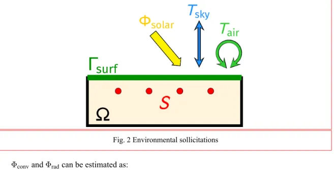
The studied structure is supposed to be submitted to environmental constraints only at its sur-rounding boundary. Other boundaries are assumed adiabatic. Three contributions are taken into account here and result in heat flux at the interface Γsurfschematized in Fig. 2: Φconvfor convective exchange with ambient air, Φskyfor radiative exchange with the sky and Φsolfor solar radiation.

Fig. 2 Environmental sollicitations

Φconvand Φradcan be estimated as:

Φconv=hconv(Tair− Tsurf) (1)

Φsky=4εσTsky3 (

Tsky− Tsurf )

(2) Where hconvis the convective exchange coefficient, a function of the wind velocity, computed here with the MacAdams correlation (Palyvos 2008). ε is the emissivity of the surrounding surface and σ the Stefan’s constant.

Four data from weather predictions are also required: air temperature, sky temperature or sky radiation density, wind velocity and solar radiation density. These data can be fetched from differ-ent forecasts sources databases such as Météo France AROME model (Seity 2011) or Copernicus Climate Data Store (CopernicusDataStore 2020) which provide application programming interface (API). When all the data are not available, it is possible to derive some quantities from literature’s correlations. For instance, the frost point can be obtained from the dew point, itself obtained from the relative humidity (Buck 1981). An example of the evolution of these parameters is shown in the numerical study case application (see Figs. 5 and 6).

2.4 Prediction of the temperature field

The temperature at the surface is here deduced from the temperature field in the structure. This one is governed by the heat equation given in Eq. (3) with boundary conditions of Eq. (4). The initial temperature is supposed to be known: T (t = 0) = T0.

(ρc)∂T

∂t − ∇ · (k∇T ) = q (3)

k· ∇T = hconv(Tair− T ) + 4εσTsky3 (Tsky− T ) + Φsol (4) A finite element formulation for spatial solving and a Crank-Nicolson scheme for temporal di-mension are used (Gartling 2010). From the knowledge of the geometry, environmental conditions and thermal properties, the temperature field can also be computed as a function of time and position in the structure.

3. Formulation of control law

In this study, the four heat sources are controlled simultaneously through the command law q(t), computed as the solution of an optimization problem. Furthermore, some constraints are imposed on the evolution and/or the maximal value of this source.

3.1 Optimization problem

The initial problem consists in computing q(t)∈ U such that T (Γtarget)≥ Tsp. To avoid an infi-nite number of solutions to this problem, the heat consumption is also minimized. This optimization problem is written under a weak formulation in Eq. (5), including the condition on the setpoint in the function to minimize. Because J ≥ 0, a solution to this problem exists.

find q = arg min ˜ q∈U J (˜q) with J (q) = 1 2∥(Tsp− T ) +_∥2 M +₂ϵ∥q∥2U (5)

where (·)+_{refers to the positive part: (x)}+_{= max (0, x).}

In a first approach, the spaceU can be considered as L2([0, ta]), the space of continuous functions

with integrable square. M = L2(Γtarget, [0, ta]) is the space of continuous and square integrable

functions in Γtarget× [0, ta]. ∥ · ∥U and∥ · ∥M are the norm for usual inner product respectively in U and M .

The minimization problem Eq. (5) includes also a residual term1₂∥(Tsp− T )+∥2_M corresponding to the respect of the condition on the setpoint and a consumption term ₂ϵ∥q∥2

The coefficient ϵ is chosen such that the solution allows to respect the constraint T (Γtarget)≥ Tsp with a fixed tolerance ∆T ≈ 0.1◦C in the present study. For a surface Γtarget of 1 m2, a value

ϵ = 10−12is used. Increasing the value of ϵ will increase the weight of the heat consumption and also increase the difference between setpoint and surface temperature when positive.

To minimize J , the gradient of this functional is computed with the adjoint state method (Lions 1971). Because ₂ϵ∥q∥2_U can be seen as a Tikhonov term (Tikhonov 1963), the problem is well-posed and such a solution exists. This method allows to get the gradient of the residual term∥(Tsp− T )∥2_M as an inner product of the spaceU where lies the heat source q. The gradient of the functional related to q can also be written as Eq. (6). For a given time t, the gradient can be deduced and is written in Eq. (7). J′(q)δq =⟨δq, (∫ S δT∗d Ω ) + ϵq⟩_U (6) ∂J ∂q(t) = ∫ S δT∗d Ω + ϵq(t) (7)

Where⟨·, ·⟩_U refers to the usual inner product inU and δT∗is the solution to the adjoint problem. This one is determined from the direct problem of equations Eq. (3) and Eq. (4) and from the expression of the functional J of Eq. (5). The adjoint problem is given in Eq. (8) and Eq. (9).

− (ρc)∂δT∗ ∂t − ∇ · (k∇δT ∗_{) =−(T} sp− T )+δΓtarget (8) k· ∇δT∗ =−(hconv+ 4εσTsky3 ) δT∗on Γsurf (9)

The system of equations Eqs. (8) and (9) has the same structure than Eqs. (3) and (4). The main difference between the two resides in considering a reverse time and a heat source at the surface with the term−(Tsp− T )+. This is the propagation in the reverse time of this source in the whole domain Ω and particularly in heating wire S that creates non-null values of the gradient of J with Eq. (6).

The same methods as for the direct problem can also be used to solve this new system, with the finite element method coupled to a Crank-Nicolson scheme for temporal dependence.

To get the optimal heat source evolution q ∈ U , the temperature field in the structure is firstly computed from an initial heat source evolution q0. Then the conjugate gradient method is applied: at each iteration adjoint problem is solved to get δT∗, the gradient J′(q)δq and also adjust heat source

q. Once the conjugate gradient has converged to ˜q, the temperature field is computed from this heat

source ˜q and the conjugate gradient is applied again. This algorithm is applied until ˜q converges or a

maximum number of iteration is reached.

3.2 Adaptation to operation constraints

In Section 3.1, it has been considered that the space in which the heat source q is defined was

U0 = L2([0, ta]). Such assumption implies a continuous evolution of q without a maximum heat

source limit. To take into account the real operation of the studied system, adaptations are considered in this section with spacesU different of U0.

3.2.1 Adaptation to time discretization

In reality, computation of temperature field is discretized with a time step, here equal to 10 min largely lower than the variations of the environmental conditions (sampled at one hour with respect to the data based used here). Heat source is also discretized with the same time grid. Integral terms are computed with linear interpolations. Moreover, to avoid too frequent commutations, heat source is sampled with a commutation time higher than the computation time step, here equal to one hour.

q is also defined as q(t ∈ [ tn, tn+1[) = qn. By noting C (tn) such a space,U = C (tn) and the

expression of the gradient given in Eq. (6) can also be reused with the inner product associated toU to obtain Eq. (10). ∂J ∂qn = ∫ tn+1 t=tn ((∫ S δT∗d Ω ) + ϵqn ) d t (10)

An adaptation can also be proposed for the case of N independent sources, each source i being on a subdomain Si ⊂ Ω with S =

⊕N

i=1Si. The spaceU becomes U = (C (tn))N and gradient of

the functional J respect to qi,nthe ith source in time interval [ tn, tn+1[ is deduced from the usual

inner product onU or directly from Eq. (10) and is written in Eq. (11). Heat sources can also be desynchronized or be considered as space dependant. Only the expression of the inner product in the spaceU needs to be known to get the gradient.

∂J ∂qi,n = ∫ ti,n+1 t=ti,n ((∫ Si δT∗d Ω ) + ϵqi,n ) d t (11)

For all these adaptations, the algorithm given at the end of Section 3.1 can be used, only the number of unknowns vary.

3.2.2 Adaptation to a maximum heat source

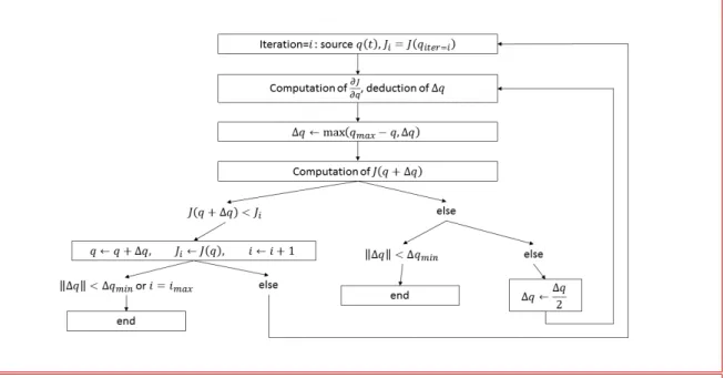
In real operation, the heat source cannot reach any value and is bounded between 0 and a given maximum value qmax. In this case, J is set to +∞ for any q /∈ U0 withU0 the subset ofU that contains the elements bounded between 0 and qmax. Gradient of J is also computed with two stages. A first evaluation comes from Eq. (12) and a correction is made to take into account the infinite values of J with Eq. (13). J′(q)δq =⟨δq, (∫ S δT∗d Ω ) + ϵq⟩_U (12) J′(q)δqn← max (0, J′(q)δqn) if qn= qmax (13) For each iteration i on the conjugate gradient method, an increment ∆q can still be computed as

qiter=i = qiter=i−1 + ∆q based on the gradient of J . However, the new value of q may not be in

U with the conjugate gradient. To stay in this set of functions, it is proposed to take ∆q such that qiter=i ∈ [0, qmax] with ∆q ← min (qmax− qiter=i−1, ∆q). The complete process is schematized in Fig. 3.

3.2.3 All or nothing operating mode

In this operating mode, the heat source can only be equal to two values at each time interval: 0 and qmax. Unlike previous operations, the number of heat source evolution sequences is not infinite: only 2Ntime _{sequences exist with N}

Fig. 3 Flowchart representing the optimization of the heat source bounded between 0 and qmax.

U ⊂ U0. There is also a solution to the optimization problem which can be obtained by computing the functional for all the elements ofU .

We propose however to use an iterative way to find a satisfying heat source evolution with a reduced number of calculations by computing the gradient of the functional J inU0 and not inU where it is not defined.

The algorithm is the following: from an initial evolution of heat source inU0, the gradient is computed inU0. Heat source for time intervals in which q = 0 and with gradient values higher than a given threshold are switched to qmax if the new value of J is lower than the previous. Then the threshold in reduced while new switches from q = 0 to q = qmaxentail decrease of J .

When the threshold reaches 0 or if there are no more switches, a similar operation is carried out for negative values of gradient. Threshold is set to a negative value and heat source switches from

qmaxto 0 for time intervals when gradient is lower than this threshold if the new value of J is lower than the previous. While J decreases, the threshold increases and new switches happen.

The gradient of the functional is then computed for this evolution of q. This process is repeated until there are no more switches. Because of the finished number of elements inU0, there is con-vergence to a solution. However, this solution may not be the optimal solution. This process is schematized in Fig. 4.

3.3 Actualization of weather forecasts

In this research paper, weather forecasts are actually weather records that come from the Me-teoNorm database (MeMe-teoNorm 2020). In a real operation, data may come from live forecasts as explained in Section 2.3. However, these data are both not exact and only available for a finite time horizon. As a consequence, data are fetched regularly (for instance each 3 hours with the model

Fig. 4 Flowchart representing the optimization of the heat source in an all-or-nothing operating mode.

AROME of Météo France (Seity 2011)) and the optimisation computation is restarted accordingly. To take into account these actualizations, the evolution of heat source is also udpated. First, heat source is computed over the time interval [0, ta]. When weather forecast is actualized, at t = ∆tact, a new evolution of q in [∆tact, ta+ ∆tact] is computed with methods presented in previous sections. To initialize the optimization process, the initial value of q is taken as the previously computed heat source on [∆tact, ta].

4. Application to a numerical study case

These different operations are applied to a study case of ten days in january for a chosen temperate oceanic climate (representative of western region in France). The associated temporal evolution of the environmental conditions is shown in Figs. 5 and 6.

Fig. 6 Environmental conditions for the selected period and location: wind speed and solar radiation.

Fig. 5 Environmental conditions for the selected period and location: air temperature and sky temperature.

Without heating, the surface temperature can be computed with the direct model. Fig. 7 shows this evolution. Temperature at the surface can decrease below 0◦C during the night which is particularly the case here during the eighth day.

0

2

4

6

8

10

time [in days]

0

20

40

60

80

x

[a

.u

.]

-5

0

5

10

15

T

[

C

]

Fig. 7 Evolution of the surface temperature at the selected location without any heating control.

Fig. 8 shows the surface temperature during the same period when heat source is activated and optimized for a setpoint equal to +4◦C without any predefined power limit. T the condition on the surface temperature higher than the setpoint with the tolerance of 0.1◦C is respected on the whole target surface.

0

2

4

6

8

10

time [in days]

0

20

40

60

80

x

[a

.u

.]

-5

0

5

10

15

T

[

C

]

Fig. 8 Evolution of the surface temperature at the selected location with an optimal heat source for a setpoint equals to +4◦C without any predefined power limit.

Results obtained are presented in Fig. 9:

• optimal control: optimal control is applied without bounding of heat source

• optimal control, qmax = 160 W : optimal control is applied with the total heat source between 0 and 160 W

• optimal control, qmax= 40 W : optimal control is applied with the total heat source between 0 and 40 W

• all-or-nothing: operation with total heat source (i. e. for the four sources) equal to 0 or 160 W

Fig. 9 Optimized heat source evolution for different operating modes, from top to down graph: optimal control without any power limitation, with qmax= 160W, with qmax= 40W

This figure also shows that operation in optimal control with and without power limit at 160 W are quite the same during the first five days for which heat source stays below the limitation.

On the contrary, during the five last days, operation with power limit entails a heat source equal to this limit most of the time. During this period, heat source evolution is closed to operation in all or nothing mode.

From the computed temperatures on Γtargetfor these various operations, the gap g with the setpoint can be evaluated. It is defined here from Eq. (14), where|Γtarget| is the area of Γtarget.

g(t) = ∫ x∈Γtarget(Tsp− T (x, t)) +_{d S} |Γtarget| (14) Fig. 10 shows the evolution of this gap for the four operation modes and without heating. Without heating and with a maximal heat source at 40 W, the surface temperature often decreases below the setpoint with gaps that can exceed 5◦C. With heat source maximum at 160 W (both optimal control and all or nothing), the gap reaches at the maximum 1◦C and less than 0.3◦C without constraint on the maximum heat source.

Δ

T

Fig. 10 Gap evolution : Temperature difference between the mean surface temperature and the set-point temperature, in log-scale.

Energy consumption are quite similar when heat source is bounded to 160 W. Without constraint on maximum heat source, consumption is higher but gap to setpoint is also reduced. For a heat source bounded at 40 W, heat consumption is lower but the objective of preventing from icing is not reached.

Table 1 Energy consumption for various operation modes

Mode Consumption [kWh] Maximum gap with setpoint [◦C] Optimal control - without power limitation 32.6 0.19 Optimal control - qmax= 160 W 25.7 1.3

Optimal control - qmax= 40 W 8.6 6.7

Optimal control - all-or-nothing: 0 or 160W 27.0 1.3

Thus, the lower the maximum heat source is, the lower the heat consumption will be, and the lower the setpoint temperature will be respected.

5. Conclusion

In this paper, control of a heating system to prevent black ice from occurring at the surface of transport infrastructures has been described. The command law relies on a direct model for the ther-mal diffusion based on the finite element method and on an adjoint state problem that has the same structure than the direct one. Solution of this adjoint problem allows to solve a minimization problem that involves energy consumption and respect of a setpoint for the surface temperature. From weather forecasts, an optimal temporal evolution for heat source can be computed.

Some adaptations caused by physical limitations of the device have been proposed and applied on a study case. Results show the possibility of using such command laws as long as weather forecasts are reliable. To go further, a validation of the approach suggested above will be performed on a mock-up. Other numerical approaches can also be studied, particularly to take into account the uncertainties around these weather forecasts and the response to the direct model. A probabilistic approach could be for example added by giving the probability for the risk of black ice occurring.

In future work, we will exploit the possibility of achieving greater energy savings by considering different setpoints like the frost temperature for optimal control.

Acknowledgements

Authors acknowledge 5th Generation Road (R5G ©) incitative research program of Université Gustave Eiffel (Previously IFSTTAR) for its overall support and The French Ministry of “Transition Ecologique et Solidaire” for also supporting part of this work under grant agreement DGITM N 17/389.

References

Asfour, S., Bernardin, F., Toussaint, E. and Piau, J.-M. (2016), “Hydrothermal modeling of porous pavement for its de-freezing.”, Applied Thermal Engineering, 107, 493–500, https://doi.org/10.1016/j.applthermaleng. 2016.06.138.

Biezma, M. V. and Schalack, F. (2007), “Collapse of steel bridge.”, J. Perform. Constr. Facil., 21, 398–405, https://doi.org/10.1061/(ASCE)0887-3828(2007)21:5(398).

Applied Meteorology, 20, 1527–1532, https://doi.org/10.1175/1520-0450(1981)020<1527:NEFCVP>2.0. CO;2.

Dai, H. L., Zhang, K. L., Xu, X. L. and Yu, H. Y. (2012), “Evaluation on the effects of deicing chemicals on soil and water environment”, Procedia Environmental Sciences, 13, 2122–2130, https://doi.org/10.1016/j. proenv.2012.01.201.

Gartling, J. N. and Reddy, D. K. (2010), “The Finite Element Method in Heat Transfer and Fluid Dynam-ics”, CRC series in computational mechanics and applied analysis. CRC Press, https://doi.org/10.1201/ 9781439882573.

Lions, J.-L. (1971), Optimal Control of Systems Governed by Partial Differential Equations, Springer-Verlag Berlin Heidelberg, Germany

Le Touz, N. and Dumoulin, J. (2019), “Study of an optimal command law combining weather forecast and energy reduction for transport structure surface de-icing by Joule effect.”, in Proceedings of Ancrisst 2019. Murray, D. M. and Ernst, U. F. W. (1976), “ An economic analysis of the environmental impact of highway deicing”, Technical Report, Municipal Environmental Research Laboratory, Office of Research and Devel-opment, U.S. Environmental Protection Agency

Pan, P., Wu, S., Xiao, Y. and Liu, G. (2015), “A review on hydronic asphalt pavement for energy harvesting and snow melting”, Renewable and Sustainable Energy Reviews, 48, 624–634, https://doi.org/10.1016/j. rser.2015.04.029.

Seity, Y., Brousseau, P., Malardel, S., Hello, G., Bénard, P., Bouttier, F., Lac, C. and Masson, V. (2011), “The AROME-France Convective-Scale Operational Model”, Monthly Weather Review, 139, 976–991, https: //doi.org/10.1175/2010MWR3425.1.

Yehia, S. A. and Tuan, C. Y. (2000), “Thin conductive concrete overlay for bridge deck deicing and anti-icing”, Transportation Research Record, 1698, 45–53, https://doi.org/10.3141/1698-07.

Copernicus Climate Change Service Climate Data Store (CDS), June 2020. https://cds.climate.copernicus.eu/. Tikhonov, A. N. (1963), “Solution of incorrectly formulated problems and the regularization method”, Doklady

Mathematics, 4, 501–504.

MeteoNorm, June 2020. https://meteonorm.com/en/.

Ifsttar mock-up at COP21 in 2015, “The Hybrid Solar Road”, Press Release, last access July 1st 2020, available at ”http://www.ifsttar.fr/fileadmin/redaction/5_ressources-en-ligne/Communication/ Espace_presse/Dossiers_de_presse/Route_solaire_En.pdf”

Le Touz N., Toullier T. and Dumoulin J.,“Infrared thermography applied to the study of heated and solar pavements: from numerical modeling to small scale laboratory experiments”, Proceedings of SPIE,dx.doi. org/10.1117/12.2262778

Palyvos, J.A (2008), “A survey of wind convection coefficient correlations for building envelope energy systems modeling”, Applied Thermal Engineering, 28, 801–808, https://doi.org/10.1016/j.applthermaleng. 2007.12.005.