GREY-BOX MODELLING FOR NATURALLY VENTILATED BUILDINGS

(1)

HAL Id: cea-01615331

https://hal-cea.archives-ouvertes.fr/cea-01615331

Submitted on 12 Oct 2017

HAL is a multi-disciplinary open access

archive for the deposit and dissemination of

sci-entific research documents, whether they are

pub-lished or not. The documents may come from

teaching and research institutions in France or

abroad, or from public or private research centers.

L’archive ouverte pluridisciplinaire HAL, est

destinée au dépôt et à la diffusion de documents

scientifiques de niveau recherche, publiés ou non,

émanant des établissements d’enseignement et de

recherche français ou étrangers, des laboratoires

publics ou privés.

Ghjuvan Faggianelli, Adrien Brun, Etienne Wurtz, Marc Muselli

To cite this version:

Ghjuvan Faggianelli, Adrien Brun, Etienne Wurtz, Marc Muselli. GREY-BOX MODELLING FOR

NATURALLY VENTILATED BUILDINGS. 14th Conference of International Building Performance

Simulation Association, Dec 2015, Hyderabad, India. �cea-01615331�

(2)

GREY-BOX MODELLING FOR NATURALLY VENTILATED BUILDINGS

Ghjuvan Antone Faggianelli

1

_{, Adrien Brun}

2

_{, Etienne Wurtz}

2

_{and Marc Muselli}

1 1

_{Universit´e de Corse, UMR CNRS 6134 SPE, Ajaccio, France}

2

_{CEA, Service Bâtiment et Systèmes Thermiques à l’INES, Le Bourget du Lac, France}

ABSTRACT

Among passive strategies to reduce energy consump-tion in buildings, we focus on natural ventilaconsump-tion, which can bring an important decrease in temperature during summer depending on climate. Despite its sim-plicity, it needs particular attention to be efficient and can be improved with building control.

In this paper, we focus on a simplified thermal model based on an electrical analogy (6R2C), coupled with a statistical airflow model and calibrated for a residen-tial building in Mediterranean climate. A full-scale experiment on this building, located in a coastal area of Corsica, allows to build and test models adapted to the case study. Both simulations and measurements are used to calibrate and test the simplified model. It is shown that the calibration phase has a great impact on model performance. An adapted calibration thus allows to reach very low errors, far bellow 0.5◦C on average, during the whole summer period. An appli-cation of this model is also proposed to control night ventilation in order to limit the number of operating cycles (windows opening and closing) and avoid over-cooling.

INTRODUCTION

Building energy simulation is commonly used for de-cision support in order to design buildings and sys-tems or estimate energy consumption. For such ap-plications, detailed models with validated software as EnergyPlus (Crawley et al., 2001) and TrnSys (Klein et al., 2010) can be relevant. However, their lack of flexibility and the high level of detail required as input are an important limitation for real-time monitoring or control. These applications, generally based on a com-promise between simulations and measurements, need flexibility and low calculation time. The model should be able to work in real-time with few data measured on site and building. Even if a reliable building model is essential, that leads to the development of simplified models which can be calibrated to measurements. For control purpose and energy saving strategies, thermal physics is generally modeled using an electrical anal-ogy. These kind of models, called grey-box models, present several advantages:

• Conservation of the physical meaning. • Clear graphical representation (RC-network). • Formulation of the system as a state space which

is easy to solve.

• Prediction of long-term energy performance with short term operation data monitoring (Wang and Xu, 2006).

The electrical analogy is based on a set of thermal resistances (R) and capacities (C) which represents the complexity of the model. We find in literature a large amount of models to describe walls and build-ing with different number of resistances and capaci-ties: 3R2C (Zayane, 2011; Coley and Penman, 1996), 6R2C (Berthou et al., 2014), 8R3C (Hazyuk et al., 2012), 3R4C (Fraisse et al., 2002), 8R7C (Wang and Xu, 2006) or even 25R10C (Kummert et al., 2001). Determining appropriate model architecture is an im-portant issue based on a compromise between com-plexity (state space dimensions and number of param-eters) and accuracy. The choice of the degree of com-plexity (model order) depends on different parameters as the type of building, systems and application. . . Here, we focus on a naturally ventilated building, lo-cated in a coastal area of Corsica. A thermal and an airflow model have been coupled in order to assess the effect of natural ventilation on air temperature. The airflow model is built with a minimal set of data by us-ing a statistical approach. Major part of this paper fo-cuses on performance evaluation of the thermal model on our case study. We aim to study the impact of the calibration phase on model reliability and robustness, which should be treated carefully (Liu et al., 2003). The set of coefficients to optimize, the length of the pe-riod, the weather conditions and internal solicitations during the calibration phase can provide significantly different results on a given structure (xRyC). It is thus required to test the model under different conditions to ensure its reliability for building control.

CASE STUDY

Building description

The building studied here is a residential building composed of twenty rooms spread over two floors with a nearly south-east orientation (Fig. 1). It is located

(3)

in a coastal zone of Corsica (France), at the Scien-tific Institute of Cargese (IESC) which has a latitude of 42.1◦, a longitude of 8.6◦ and an altitude of about 13m. Each room of the building is identical and in cross-ventilation configuration.

In this study, a second floor room with the following characteristics (from the inside to the outside) has been instrumented:

• The external wooden walls have a high level of insulation with 19 mm gypsum board, 50 mm wood fibre, 120 mm cellulose wadding and 16mm wood panel.

• The partition walls have a high thermal inertia with 180mm high density concrete.

• The partition floor is made of 150 mm high den-sity concrete.

• The roof is made of 180 mm of high density con-crete, 180mm of cellulose wadding and 19 mm gypsum board.

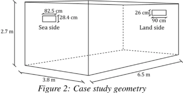
Figure 1: Residential building of IESC Here, we consider the configuration presented in Fig. 2. The two openings on opposite walls have the same area and the same height above ground which simplify the natural ventilation behavior, assuming an unidirectional flow based on the virtual stream tube phenomenon (Murakami et al., 1991). The airflow model thus only takes into account the wind effect and the thermal buoyancy is neglected (British Standards Institution, 1991). 82.5 cm 28.4 cm 2.7 m 3.8 m 6.5 m 26 cm 90 cm Sea side Land side

Figure 2: Case study geometry

Site and building instrumentation

To test or build new models it is necessary to obtain reliable data. However, a complete building energy model requires numerous boundary conditions (tem-perature, humidity, wind speed and direction, solar

ra-diations. . . ). This includes two categories of measure-ments:

• The weather conditions which affect the building. • The building response to the solicitations (air

temperature, airflow rate. . . ).

Depending on the accuracy expected, the set of quired measurements is variable. It is possible to re-duce this instrumentation using different models and correlations to get all the data required. Here, the aim is to get a simple model to optimize windows control during warm season, in an occupied building. It is thus important to use the least possible sensors on site and building.

For this experiment, we only measure the following data:

• Global horizontal irradiance (1 pyranometer, Kipp & Zonen CMP6);

• Outside temperature (1 temperature probe, Vaisala HMP110 with solar radiation shield); • Inside temperature (1 Resistance thermometer,

Pt100 with four-wire configuration);

• Wind speed and direction (1 ultrasonic anemome-ter, Vaisala WMT52).

This instrumentation has been set up during a period of nearly two summer months, from July 02 to August 19 with a 20s time step. It constitutes the minimal set of data, based on only 4 sensors, which will be used to calibrate and test the simplified model.

For the missing data, we use the following correla-tions:

Solar radiations

Direct and diffuse components must be deduced from global irradiance. Many empirical and parametric models allow to perform direct and diffuse decom-position but they may require numerous parameters (Wong and Chow, 2001). Simple clear sky models, as Erbs’ model (Erbs et al., 1982), only require global irradiance but lead to higher uncertainties. However, they appear to be an interesting approach to reduce the number of sensors and still give good results in our latitudes (Notton et al., 2006).

Finally, we rely on EnergyPlus software (Crawley et al., 2001) to preprocess the transmitted and incident solar radiation to the zone and exterior walls.

Sky temperature

The sky temperature is estimated from the outside tem-perature,To, by Swinbank model (Swinbank, 1963):

Tsky = 0.0552 To1.5 (1)

Airflow rate

To calculate the airflow rate with a minimum informa-tion, building energy simulation software often pro-pose empirical models. However, they are based on parameters which can be difficult to evaluate (pressure and discharge coefficient) and present very high un-certainties (Freire et al., 2013). Here, we use an

(4)

artifi-cial neural network based on wind speed and direction measurement and especially built for this experimental configuration.

BUILDING THERMAL MODEL

Model presentation

Thermal physics within the zone is modelled using an electrical analogy. We propose a rather simple second order lumped model developed under MATLAB envi-ronment. Its structure (6R2C) is presented in Fig 3.

Φi b b b bb bb b b b b Rs,i Rm,12 Rm,22 Rs,e Φs,i Φm Φs,e Rf i Ci Cm Ti Ts,i Tm Ts,e Te TGLO,e RGLO,e 1 Figure 3: 6R2C model

The analogy is based on the following assumptions: • All walls are assimilated to one wall with

equiv-alent propertiesCm,Rm.

• This wall is represented by a 2R1C model where the 2 resistances,Rm,12andRm,22(withRmthe

total resistance), are between both sides of the wall capacityCm.

• Absorbed solar radiations for the external walls are integrated in the flowΦs,e, and applied on the

external node of the equivalent wall.

• Heat transfer through low inertia elements (glaz-ing, doors and ventilation) are represented by Rf i.

• Internal loads and a part of solar radiations through glazing are integrated in the flowΦi.

• Φs,i represents the flow injected into the inner

surface of the building. It integrates the solar flow through glazing absorbed by inner surface as well as the radiative part of the internal loads. • Φmis a flow injected inside the wall, allowing to

model an active floor/wall component. As it is not used during summer, it has a value of zero in this study.

• Convective heat transfer between internal air and inner wall surface are integrated inRs,i.

• Convective heat transfer between external air and outer wall surface are integrated inRs,e.

• Infrared radiation between external wall and en-vironment (long wavelength) is represented by RGLO,e.

The system of equation is derived from heat balance on air volume (i), on inner wall surface (s, i), on inner

wall (m) and on the outer wall surface (s, e):

Ci dTi dt = Te− Ti Rf i +Ts,i− Ti Rs,i + Φi (2) 0 = Ti− Ts,i Rs,i +Tm− Ts,i Rm,12 + Φs,i (3) Cm dTm dt = Ts,e− Tm Rm,22 +Ts,i− Tm Rm,12 + Φm(4) 0 = Tm− Ts,e Rm,22 +Te− Ts,e Rs,e (5) +TGLO,e− Ts,e RGLO,e + Φs,e With: • Rm,12= 1/(UmSm) × (1 − γm) • Rm,22= 1/(UmSm) × γm • Rs,i= 1/(hciSm) • Rs,e= 1/(hceSm) • RGLO,e= 1/(hr Sm)

Finally, we also use a coefficientγCLOto spread the

solar gain between internal air node (Φi) and inner

wall surface (Φs,i).

The values of all these parameters (Um,hci,hce,hr,

γm and γCLO) and some resistances and capacities

(Rf i, Cm and Ci) are defined by model calibration

which will be developed in further section. This rep-resents a total of 9 parameters.

In order to consider the effect of variable airflow rate, we integrate a specific flowΦv:

Φv(t) = [To(t) − Ti(t − 1)] Qv(t) Cpairρair (6)

Where Qv is the airflow rate in m3_.h−1_, _Cp air the

specific heat capacity of air in J.(kg.K)−1 _and_ρ air

the density of air inkg.m−3_.

A coefficientγvis used to spread it between the

inter-nal air node and the inner surface of the room. This flow is only considered when the airflow rate is vari-able. In this condition, the coefficientγv is also

cali-brated, increasing the number of parameters to 10. The system is then converted into a state-space rep-resentation and the resolution is given by an implicit Euler method:

dX

dt = Γ × X + ξ × ST (7) Wheret is the time, X a vector of state function, ST a

vector of solicitations andΓ and ξ are coefficient ma-trices.

Model performances

To test the model performances, it is necessary to have reliable data during a sufficient period and various conditions. The data from the experimentation will be used to test the model under real conditions but do not allow to properly assess the model performances. For this purpose, we will rely on EnergyPlus which is

(5)

a validated building energy simulation software (Hen-ninger et al., 2004). It presents the advantage to al-low the control of many parameters during the simula-tion such as weather condisimula-tions, internal loads, airflow rate. . . and thus to test the model with the desired con-ditions. Here, it will be used as a reference to calibrate the simplified RC model and calculate the error. The EnergyPlus model (which will be called EP model) is a detailed model of one room (Fig.2) with adiabatic boundary conditions for internal walls. When the building is not ventilated, we consider an air infiltration of 0.2ACH. The weather file used for the simulation is based on a typical meteorological year (T M Y 2 file) from the city of Ajaccio (about 20 km from Cargese).

In this paper, we focus on some of these tests which are representatives of the overall results and allow to draw some conclusions. For each test, we use common parameters for the following points:

• Tests are performed on extended summer period: from June 01 to September 30.

• The calibration of the RC model is done during 15 days: from June 01 to June 15, with aP SO al-gorithm (Particle Swarm Optimization) based on M SE error function (Mean Squared Error). • The simulations are run with a 5-minute time

step.

Constant airflow rate

As a first step, the RC model is tested with a constant airflow rate of 3ACH, to assess the impact of weather and internal loads variations. For the Case 1, we con-sider the following internal loads with a daily profile:

• Occupant: 70 W from 10pm to 8am, 120 W from 8am to 9am and from 7pm to 10pm.

• Lighting: 60 W from 7am to 9am and from 8pm to 11pm.

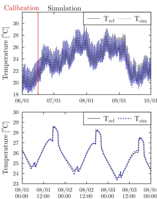
• Electric equipment: 250 W from 7pm to 10pm. The Fig. 4 presents the comparison of the two mod-els during the whole period (top) and with a zoom on a few days (bottom) to clearly show the temperature profile. There are important variations due to weather conditions with lower temperatures at beginning and end of the period: between 18 and 24◦C from 06/01 to 06/15 and from 09/10 to 10/01 while the temperature can reach 30◦C in midsummer. Moreover, important internal loads during evenings also affect the temper-ature profile. This first case is thus representative of weather conditions and internal loads effects on tem-perature.

In terms of errors, we observe aM AE of 0.07◦_{C for}

the calibration and 0.20◦C for the simulation. These results are thus very satisfying and show the capability of the simplified model to take into account variations in weather conditions and internal loads. However, a daily profile of internal loads is used in this case, which simplify the model calibration. To assess the

Figure 4: Comparison between reference EP model and simplified RC model on Case 1

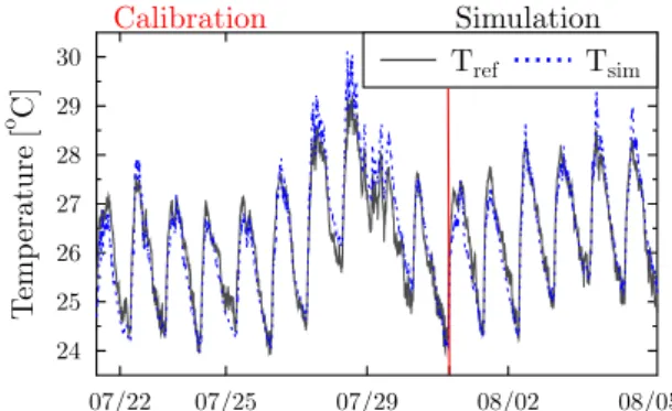
least favorable situation, Case 2, we use the same pa-rameters as in Case 1 but we do not take into account the internal loads until 08/01, during simulation. As observed in Fig. 5, this leads to a significant loss of accuracy as soon as the internal loads are added in the simulation. Even if the two models present a similar trend, an error up to 2◦C is regularly reached.

To improve this result, it is necessary to take into ac-count internal loads during calibration. However, a real building may present variations in its use over time and we cannot consider only one daily or weekly profile. A compromise could be achieved by includ-ing different types of internal loads in the calibration phase: periods with no internal loads (building not oc-cupied) and variables internal loads during day and night. In Case 3, we propose a simplified example to show the interest of this method:

(6)

• From 06/01 to 06/10 (begin of calibration): no internal loads.

• From 06/11 to 06/15 (end of calibration): internal loads same as for Case 1.

• From 06/16 to 07/31 (begin of simulation): no internal loads.

• From 08/01 to 09/30 (end of simulation): internal loads same as for Case 1.

Here, we consider only 4 days with internal loads dur-ing calibration. Durdur-ing simulation, they will only ap-pear one and a half months later. It is thus an interest-ing case to assess the robustness of the model.

The Fig. 6 shows that this time, the RC model fits the EP model with a better accuracy and reaches aM AE of 0.10 ◦C for the calibration and 0.17 ◦_{C for the}

whole simulation. On 08/01, when we add internal loads in the simulation, the model is now able to fol-low the changes in temperature profile.

These first tests highlight the importance of the cali-bration phase. A relevant calicali-bration is essential to get a reliable model which can be used on a long period. Moreover, Case 3 shows that a degree of freedom is still possible as long as we consider realistic internal loads according to the building use.

Controlled ventilation

As the simplified model gives satisfying results with constant airflow, we can now focus on the effects of a variable rate in model performances. Before consider-ing natural ventilation, we propose in Case 4 to asses a controlled ventilation system with the following rates:

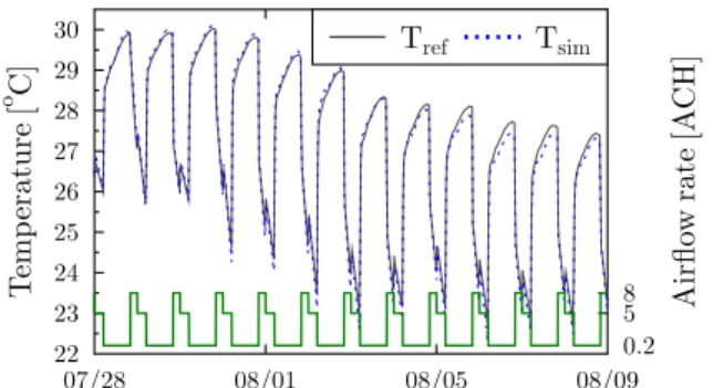
• 0.2 ACH from 7am to 10pm. • 8 ACH from 10pm to 2am. • 5 ACH from 2am to 7am.

We also introduced some constant internal loads (60W for lighting and 100 W for occupants) to sim-ulate the presence of an occupant in the building. To present the trends of the the temperatures, we still focus on the period of 07/28 to 08/09, around the mid-dle of the simulation (Fig. 7). Here, theM AE reaches 0.06◦C for the calibration and 0.15◦_{C for the whole}

simulation. As for internal loads, the variations of

air-Figure 7: Comparison between reference EP model and simplified RC model on Case 4

flow rate do not affect the model accuracy if they are taken into account during the calibration phase. Natural ventilation

To conclude these tests, we focus on natural ventila-tion. In Case 5, we consider that the building is always ventilated with a realistic airflow rate directly related to the wind profile (speed and direction) and to the opening geometry (position and surface). This leads to very variable airflow rates, from near 0 to 40ACH which will have a great impact on temperature. Inter-nal loads are also the same as in Case 1 but their impact will be low here, due to the continuous use of natural ventilation.

The Fig. 8 shows that the RC model is still very accu-rate even with an airflow accu-rate fluctuating widely. Here, we observe a very low error with aM AE of 0.09◦_C

for the calibration and 0.11◦C for the simulation. This result thus gives confidence in its use for natural ven-tilation control. However, we still have to take care of the calibration phase. To control windows opening and closing, it will be required to use different peri-ods during calibration: with and without internal loads and with and without airflow rate with different and realistic variations. As an example, we show in Fig. 9 (Case 6) the effect of closing windows during simula-tion while the model is only calibrated with continuous natural ventilation.

(7)

closed, we observe an important error increasing over time. In the end of August this error exceeds 4 ◦C. However, from 09/01 when the windows are opened again, the error decreases, becoming insignificant a few days after. As the natural ventilation brings a high airflow rate with important heat transfer, we observe a fast convergence of the simulation. This confirms the robustness of the simplified model when used with known phenomena, included in calibration. As for internal loads, the effect of calibration is critical for model performance. In the same way, the error in this example could be greatly reduced by including a short period without ventilation during calibration.

Experimental study

There is an important difference between using a building model from a simulation software where all parameters can be known and a real building with many uncertainties. Indeed, it will be necessary to use real measurements and some correlations which will add errors in the model. Here, we focus on the real building and measurements presented above. The aim will be to calibrate the RC model with these data and to compare its response with the temperature measured in the room.

The main sources of uncertainties are supposed to be the effect of solar radiation, estimated with only global horizontal irradiance, and of airflow rate, estimated with a statistical model based on wind speed and di-rection (Faggianelli et al., 2015). These kinds of un-certainties are unavoidable in real case studies. It is thus interesting to assess their impact on model per-formance. As we do not have a long period of us-able data, we use 10 days for model calibration and 6 days of simulation. This represents 5 fewer days for model calibration in comparison with the previous tests, which is also less favorable. A last change con-cerns the time step, which is now set to one minute (obtained by average of the 20s measurements). For this test (Fig. 10), we observe aM AE of 0.39◦_C

for the calibration and 0.31 ◦C for the simulation. Even if the errors are higher than those obtained by comparison with EnergyPlus, these results are still sat-isfying considering all the uncertainties (error bellow

Figure 10: Comparison between real measurements and simplified RC model

0.5◦C on average). Although this test does not allow to assess the performance on a whole summer period, it is thus promising for using the simplified model in order to control natural ventilation in the building.

BUILDING CONTROL APPLICATION

To highlight the possibilities of use of the model, we present an example for night ventilation control in the residential building of IESC. The aim will thus be to monitor the indoor temperature in order to ensure thermal comfort. This requires to control windows opening for natural ventilation while taking care to not overcool the building. When there is no risk of overcooling, it may be better to use more simple ap-proaches such as real time measurement of the temper-ature difference between outside and inside the build-ing. We will thus focus here on the problem of au-tomatic control on a specific case, chosen to illustrate this application.

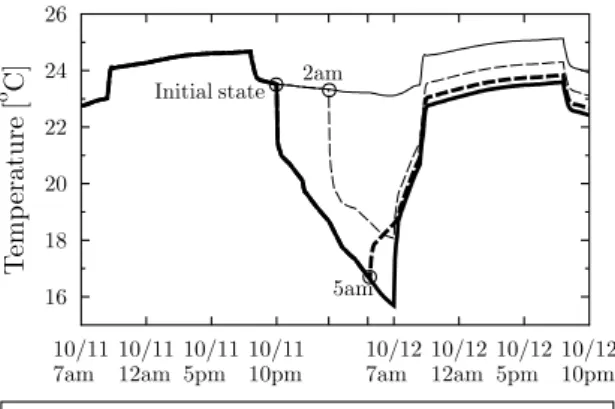
The main issue in automatic systems is the number of operating cycles. A high number of cycles per night will decrease the lifetime of the system and will induce discomfort for building occupant (engine noise). The use of a simplified model with predictive data is gener-ally a good way to provide energy efficient and com-fortable building (Ma et al., 2012; Candanedo et al., 2013). Here, the model can be used to minimize the number of operating cycles and approach a setpoint temperature at a given time. In this example, we allow only one change in windows state (opening or closing) and we want to reach a setpoint temperature of 18◦C at 7am. From predictive data (weather conditions), the model is able to calculate the best time to change the windows state by means of successive simulations. If we want to use it in the evening, around 10pm, we need a forecast horizon of about 9h. These data can be obtained from some weather data providers or by local predictive models. As the use of predictive data introduces more uncertainties in the model, we will calculate the time with a low resolution, in hour. For this example, we will use EnergyPlus to generate a set of data instead of using real predictive data.

(8)

October 12. To provide a more visual case, we use the following assumptions for the simulation:

• Important internal loads during day: 200 W (electric equipment) from 9am to 10pm.

• No night ventilation from October 01 to October 10: low internal loads dissipation and heat stored in walls.

• The control is used from October 11, 10pm to Oc-tober 12, 7pm and the windows are closed before and after this period.

• Important airflow rate between October 11 and October 12 to ensure an efficient night ventila-tion.

Figure 11: Effect of different control strategies

In Fig. 11, we present 4 possibilities. Two of them are the solutions calculated by the model:

• Windows opened at 10pm and closed at 5am. • Windows closed at 10pm and opened at 2am. The other two are obtained without control, with win-dows open or closed all night long. The results ob-tained with the different possibilities are resumed in Table 1. The two solutions given by the model are Table 1: Temperature depending on the strategy used

Windows state 10/12 at 7am Open 15.7 Open then closed at 5am 18.5 Closed 23.1 Closed then open at 2am 18.1

acceptable with a temperature close to the setpoint at 7am (differences between 0.1 and 0.5 ◦C). Without control, the temperature will be too low (2.3 ◦C less than the setpoint) or too high (5.1 ◦C more than the setpoint).

As the building has an important inertia, one night of natural ventilation will not be sufficient to remove heat in walls and store cold instead. This is clearly observed at 7am: when the windows are closed, the temperature increases quickly. In addition to show the benefit of control, this example highlights the interest

of using an adapted strategy at the earliest to avoid this kind of situation.

CONCLUSION

This paper is focused on calibration and test of a grey-box thermal model coupled to a black-grey-box airflow model. These models represent a naturally ventilated room and could be used for building control optimiza-tion applicaoptimiza-tions. A comparison with the validated software EnergyPlus has shown the importance of the calibration phase which impacts directly the model performance. An adapted calibration allows to reach very low errors, far bellow 0.5◦C on average, during the whole summer period. This result has been ob-served on different cases with important variations on weather conditions, internal loads and airflow rates. A full-scale experiment on a real building located in a coastal area of Corsica also confirmed the robustness of the simplified model even if confronted to many sources of uncertainty.

The results presented in this paper are thus promising and show the interest of this approach to control and optimize natural ventilation in buildings. An example of application has been also proposed for night venti-lation control in order to limit the number of windows opening/closing cycles and avoid overcooling. The de-velopment of adapted algorithms for real time and pre-dictive control appears as a perspective of this study.

REFERENCES

Berthou, T., Stabat, P., Salvazet, R., and Marchio, D. 2014. Development and validation of a gray box model to predict thermal behavior of occupied office buildings. Energy and Buildings, 74:91–100. British Standards Institution 1991. Code of practice

for ventilation principles and designing for natural ventilation. BS 5925. London.

Candanedo, J. A., Dehkordi, V. R., and Lopez, P. 2013. A control-oriented simplified building mod-elling strategy. In Proceedings of Building Simula-tion 2013: 13th Conference of InternaSimula-tional Build-ing Performance Simulation Association.

Coley, D. A. and Penman, J. M. 1996. Simplified ther-mal response modelling in building energy manage-ment. paper III: demonstration of a working con-troller. Building and Environment, 31(2):93–97. Crawley, D. B. et al. 2001. EnergyPlus: creating

a new-generation building energy simulation pro-gram. Energy and Buildings, 33(4):319–331. Erbs, D. G., Klein, S. A., and Duffie, J. A. 1982.

Es-timation of the diffuse radiation fraction for hourly, daily and monthly-average global radiation. Solar Energy, 28(4):293–302.

Faggianelli, G. A., Brun, A., Wurtz, E., and Muselli, M. 2015. Assessment of different airflow modelling

(9)

approaches on a naturally ventilated Mediterranean building. Energy and Buildings.

Fraisse, G., Viardot, C., Lafabrie, O., and Achard, G. 2002. Development of a simplified and accurate building model based on electrical analogy. Energy and Buildings, 34(10):1017–1031.

Freire, R. Z., Abadie, M. O., and Mendes, N. 2013. On the improvement of natural ventilation models. Energy and Buildings, 62:222–229.

Hazyuk, I., Ghiaus, C., and Penhouet, D. 2012. Op-timal temperature control of intermittently heated buildings using model predictive control: Part II – control algorithm. Building and Environment, 51(0):388–394.

Henninger, R. H., Witte, M. J., and Crawley, D. B. 2004. Analytical and comparative testing of Ener-gyPlus using IEA HVAC BESTEST e100e200 test suite. Energy and Buildings, 36(8):855–863. Klein, S. et al. 2010. TRNSYS 17: A Transient

Sys-tem Simulation Program, Solar Energy Laboratory. University of Wisconsin, Madison, USA.

Kummert, M., Andr´e, P., and Nicolas, J. 2001. Op-timal heating control in a passive solar commercial building. Solar Energy, 69:103–116.

Liu, M., Claridge, D., Bensouda, N., Heinemeier, K., Lee, S., and Wei, G. 2003. Manual of procedures for calibrating simulations of building systems. Techni-cal report, California Energy Commission.

Ma, Y., Kelman, A., Daly, A., and Borrelli, F. 2012. Predictive control for energy efficient buildings with thermal storage: Modeling, stimulation, and experi-ments. IEEE Control Systems, 32(1):44–64. Murakami, S., Kato, S., Akabayashi, S., Mizutani, K.,

and Kim, Y.-D. 1991. Wind tunnel test on velocity-pressure field of cross-ventilation with open win-dows. In ASHRAE Transactions, volume 97, pages 525–538, New York.

Notton, G., Poggi, P., and Cristofari, C. 2006. Pre-dicting hourly solar irradiations on inclined sur-faces based on the horizontal measurements: Per-formances of the association of well-known math-ematical models. Energy Conversion and Manage-ment, 47(13–14):1816–1829.

Swinbank, W. C. 1963. Long-wave radiation from clear skies. Quarterly Journal of the Royal Mete-orological Society, 89(381):339–348.

Wang, S. and Xu, X. 2006. Simplified building model for transient thermal performance estimation using GA-based parameter identification. International Journal of Thermal Sciences, 45(4):419–432. Wong, L. and Chow, W. 2001. Solar radiation model.

Applied Energy, 69(3):191–224.

Zayane, C. 2011. Identification d’un modèle de com-portement thermique de bâtiment à partir de sa courbe de charge. PhD thesis.