HAL Id: hal-01969722
https://hal.archives-ouvertes.fr/hal-01969722
Submitted on 14 Jan 2019
HAL is a multi-disciplinary open access
archive for the deposit and dissemination of
sci-entific research documents, whether they are
pub-lished or not. The documents may come from
teaching and research institutions in France or
abroad, or from public or private research centers.
L’archive ouverte pluridisciplinaire HAL, est
destinée au dépôt et à la diffusion de documents
scientifiques de niveau recherche, publiés ou non,
émanant des établissements d’enseignement et de
recherche français ou étrangers, des laboratoires
publics ou privés.
Spectroscopic determination of kinetic parameters for
frequency sweeping Alfvén eigenmodes
Maxime Lesur, Y. Idomura, K. Shinohara, X. Garbet
To cite this version:
Maxime Lesur, Y. Idomura, K. Shinohara, X. Garbet. Spectroscopic determination of kinetic
param-eters for frequency sweeping Alfvén eigenmodes. Physics of Plasmas, American Institute of Physics,
2010, 17 (12), pp.122311. �10.1063/1.3500224�. �hal-01969722�
Spectroscopic determination of kinetic parameters for frequency sweeping
Alfvén eigenmodes
M. Lesur,1,2Y. Idomura,1K. Shinohara,3X. Garbet,2and the JT-60 Team3
1
Japan Atomic Energy Agency, Higashi-Ueno 6-9-3, Taitou, Tokyo 110-0015, Japan 2
IRFM, Commissariat à l’Energie Atomique, F-13108 Saint Paul Lez Durance, France 3
Japan Atomic Energy Agency, Mukouyama 801-1, Naka, Ibaraki 311-0193, Japan
共Received 29 March 2010; accepted 21 September 2010; published online 17 December 2010兲 A method for analyzing fundamental kinetic plasma parameters, such as linear drive and external damping rate, based on experimental observations of chirping Alfvén eigenmodes, is presented. The method, which relies on new semiempirical laws for nonlinear chirping characteristics, consists of fitting procedures between the so-called Berk–Breizman model and the experiment in a quasiperiodic chirping regime. This approach is applied to the toroidicity induced Alfvén eigenmode 共TAE兲 on JT-60 Upgrade 共JT-60U兲 关N. Oyama et al., Nucl. Fusion 49, 104007 共2009兲兴, which yields an estimation of the kinetic parameters and suggests the existence of TAEs far from marginal stability. Two collision models are considered, and it is shown that dynamical friction and velocity-space diffusion are essential to reproduce nonlinear features observed in experiments. The results are validated by recovering measured growth and decay of perturbation amplitude and by estimating collision frequencies from experimental equilibrium data. © 2010 American Institute of Physics. 关doi:10.1063/1.3500224兴
I. INTRODUCTION
In an ignited tokamak, the confinement of␣-particles is critical to prevent damages on the first wall and to achieve break even. A major concern is that high energy ions can excite plasma instabilities in the frequency range of Alfvén eigenmodes 共AEs兲, which significantly enhance their trans-port. Ever since the recognition of this issue in the 1970s, considerable progress has been made in the theoretical un-derstanding of the principal Alfvénic instabilities. However, the estimation of the mode growth rate␥is complex, and the question of their stability in ITER 共Ref. 1兲 remains to be
clarified. Linear theory predicts that the toroidicity induced Alfvén eigenmode2 共TAE兲 is stable when the continuous damping of the background plasma exceeds the drive of fast particles. Thus, accurate estimations of fundamental kinetic parameters such as the linear drive␥Land the damping rate
␥d are needed, especially if the system is close to marginal
stability, where ␥ is sensitive to small variations. For this class of instabilities, the growth rate can be estimated either by linear stability codes such asPENN,3TASK/WM,4NOVA-K,5 or CASTOR-K共Ref. 6兲 or by gyrokinetic or drift-kinetic
per-turbative nonlinear initial value codes such asFAC共Ref.7兲 or
HAGIS.8The analysis requires internal diagnostics that are not always available. The global damping involves complicated mechanisms with details still under debate. Experimentally, ␥d can be estimated by active measurements of externally
injected perturbations.9,10 However, the applicability of this technique is limited to dedicated experiments, and this pre-vents robust linear predictions of the stability of AEs. More-over, the existence of unstable AEs in a regime where linear theory predicts␥⬍0, or subcritical AEs, has not been ruled out. Therefore, nonlinear analysis is needed to assess the stability.
In general, these instabilities are described in a
three-dimensional 共3D兲 configuration space. However, near the resonant surface, it is possible to obtain a new set of vari-ables in which the plasma is described by a one-dimensional 共1D兲 Hamiltonian in two conjugated variables11–14
if we as-sume an isolated single resonance. In this sense, the problem of AEs is homothetic to a simple 1D single mode bump-on-tail instability. The so-called Berk–Breizman 共BB兲 problem11,12,15 is a generalization of the bump-on-tail prob-lem, where we take into account an external wave damping accounting for background dissipative mechanisms at a rate ␥dand a collision operator. Observed quantitative similarities
between BB nonlinear theory and both global TAE simulations13,16and experiments17,18are an indication of the validity of this reduction of dimensionality.
A feature of the nonlinear evolution of AEs, the fre-quency sweeping 共chirping兲 of the resonant frequency by 10%–30% on a timescale much faster than the equilibrium evolution, has been observed in the plasma core region of tokamaks JT-60U,19 DIII-D,20 the Small Tight Aspect Ratio Tokamak,21 the Mega Amp Spherical Tokamak 共MAST兲,16 and the National Spherical Torus Experiment22 and in stell-erators such as the Compact Helical Stellerator,23 and the Large Helical Device.24 In general, two branches coexist, with their frequency sweeping downwardly共down-chirping兲 for one, upwardly共up-chirping兲 for the other. In most of the experiments, chirping events are quasiperiodic, with a period of the order of a millisecond. In many experiments, asym-metric chirping has been observed, with the amplitude of down-chirping branches significantly dominating up-chirping ones.
Qualitatively similar chirping modes are spontaneously generated by the BB model, and theory relates the time evo-lution of the frequency shift with␥Land␥d.25 In this work,
we identify a regime where chirping events are
cal. This regime exists whether the collision model is annihilation/creation type or takes into account dynamical friction and velocity-space diffusion. We recall the equations of the BB model and numerically investigate nonlinear chirping features for both collision operators in Sec. II. In a previous work,26 we showed that the nonlinear time evolu-tion of chirping in 1D simulaevolu-tions can be used to retrieve fundamental kinetic parameters with a good precision, which suggests that it is possible to retrieve kinetic parameters from experimental observations of chirping AEs. We propose a new method to estimate␥L,␥d,␥, and collision frequencies
from the spectrogram of magnetic field variations measured by a Mirnov coil at the edge of the plasma. This method, which relies on a fitting of normalized chirping characteris-tics between the experiment and BB simulations, is described and applied to JT-60U AE experiments in Sec. III. We show that the BB model can successfully reproduce features ob-served in the experiment only if the collision operator in-cludes drag and diffusion terms. In Sec. IV, an independent estimation of collision frequencies is obtained from experi-mental equilibrium measurements, and compared with the values obtained with our fitting procedure.
II. NONLINEAR FREQUENCY SWEEPING A. The Berk–Breizman model
We adopt a perturbative approach and cast the so-called BB model27in a reduced form that describes the time evolu-tion of the beam particles only.28The main hypothesis of this model is that the bulk particles interact adiabatically with the wave so that their contribution to the Lagrangian can be expressed as a part of the electric field. In this model, the real frequency of the wave is imposed as =p, where p
⬅共4n0q2/m兲1/2 is the plasma frequency 共in cgs units兲, q and m are the electronic charge and mass, and n0is the total plasma density. The evolution of the beam distribution, f共x,v,t兲, is given by the kinetic equation
f t +v f x+ qE˜ m f v=C共f − f0兲, 共1兲
whereC共f − f0兲 is a collision operator described below, f0共v兲 is the initial distribution function, and the pseudoelectric field E˜ is defined as
E
˜ 共x,t兲 ⬅m
q关Q共t兲cos共兲 − P共t兲sin共兲兴, 共2兲 where⬅kx−pt.
In the definition of E˜ , we assume a single mode of wave number k, reflecting the situation of a low toroidal mode number Alfvèn eigenmode, whose excited spectrum is usu-ally discrete. The evolution of the pseudoelectric field is given by dQ dt = − p 3 2n0
冕
f共x,v,t兲cos共兲dxdv −␥dQ, 共3兲 dP dt = 3p 2n0冕
f共x,v,t兲sin共兲dxdv −␥dP, 共4兲where an external wave damping has been added to model all linear dissipation mechanisms of the wave energy to the background plasma, which are not included in the previous equations. In the initial condition, we apply a small pertur-bation, f共x,v,t=0兲= f0共v兲共1+⑀cos kx兲, and the initial values of Q and P are given by solving the Poisson equation. We refer to Eqs.共1兲–共4兲as the␦f BB model, in opposition to the full-f BB model studied in Ref.26.
We define and ␥ as the real frequency and linear growth rate of the wave, respectively, including contributions of external damping and collisions. In the collisionless case, one can see from the linear dispersion relation that =p
only if f0 is symmetric around the resonant velocity, vR
⬅/k. Since we assumed=pfrom the start, we consider
only such distributions, for the model to be self-consistent. The velocity distribution of beam particles in the initial con-dition, f0, is shown in Fig.1共a兲for typical simulation param-eters. A constant slope is imposed between v = −vc and v
=vc. The zero average ensures that the plasma frequency is
not perturbed by the beam density. Smooth joins between the constant gradient region and the large velocity regions are necessary to prevent numerical oscillations atv⬇ ⫾vc. For
␥/Ⰶ1, the dispersion relation yields
␥=␥L0−␥d, 共5兲 where ␥L0⬅ 2n0 p 3 k2
冏
f0 v冏v=v
R . 共6兲Let us define␥L as the linear growth rate in the absence of
collisions and external dissipation. Note that in general,␥L0
and␥Lare slightly different. In this paper, we use␥L0solely
as a measure of the slope of the initial velocity distribution. We consider two collision models. On the one hand, a large part of existing theory takes into account collisions in the form of a Krook operator,29
-0.5 0 0.5 -vc vc -1 0 1 (v-vR) / vR (a) t = 0 Krook Drag/Diffusion -0.1 0 0.1 -0.1 0 0.1 10-2 10-1 100 0 2 4 ωb /γL νefft (b) Krook Drag/Diffusion
FIG. 1. 共Color online兲 共a兲 Distribution function normalized to
n0␥L0/共冑2vRp兲. Solid line is the initial condition, dashed lines are for
efft = 2.共b兲 Time evolution of the bounce frequency. Parameters are ␥L0
= 0.1,␥d= 0.05, andeff= 0.02. In the drag/diffusion case,d/f= 3.
CK共f − f0兲 = −a共f − f0兲, 共7兲 which is a simple model for collisional processes that tend to recover the initial distribution at a rate a, including both
source and sink of energetic particles. On the other hand, a more realistic collision operator, the one-dimensional projec-tion of a Fokker–Plank operator,30includes a dynamical fric-tion共drag兲 term and a velocity-space diffusion term,
CFP共f − f0兲 = f 2 k 共f − f0兲 v + d 3 k2 2共f − f 0兲 v2 . 共8兲
Another large part of existing theory deals with the latter operator in the absence of drag共f= 0兲. Investigations of the
effects of dynamical friction are fairly recent.30We define the effective collision frequency as eff⬅a in the Krook case
andeff⬅d3/␥L02 in the case with diffusion.
In a previous work,26we developed and validated a 1D semi-Lagrangian Vlasov code, referred to as COBBLES, in-cluding a Krook operator and extrinsic dissipation, capable of long-time, accurate nonlinear simulations of both full-f and␦f BB models. In this paper, we use the ␦f version of COBBLESto investigate the nonlinear characteristics of chirp-ing solutions. For this work, a collision operator with drag and diffusion is implemented. We confirmed quantitative agreement of nonlinear steady-state solutions between the extended code and Ref.30. Detailed verification will be in-cluded in a separate publication. Both in our simulations and in the remainder of this paper, time is normalized top
un-less some physical unit is explicitly given. When we com-pare simulation and experimental results, we simply renor-malize time by the measured AE linear frequency. In this work, all simulations are performed with Nx⫻Nv= 64
⫻2048 grid points and a time-step width 0.05. The large number of grid points in velocity space is necessary to avoid recurrence effect during the quiescent phase between two chirping events.
B. Chirping characteristics
The nonlinear behavior of an instability is determined by a competition among the drive by resonant particles, the ex-ternal damping, the particle relaxation that tends to recover the initial positive slope in the distribution function, and par-ticle trapping that tends to smooth it. Chirping solutions arise in a low collision regime when hole and clump structures11 are formed in phase-space. They belong to a chaotic regime, and each chirping event is slightly different. The velocity distribution after nonlinear saturation shown in Fig.1共a兲 il-lustrates the fact that several holes and clumps with different amplitudes can coexist. In this work, we are interested in the nonlinear chirping characteristics, averaged over a significant number of chirping events. In particular, in our simulations, the first chirping event is observed to stand out from the statistics, with a larger extent of chirping—up to twice as much as any other one of the following series of repetitive chirping. This may be due to the fact that the first chirping benefits from a perfectly constant velocity-slope, while fol-lowing events are subject to the interference of phase-space structures that remain from previous chirping events. Since
the latter condition seems more experimentally relevant, the first chirping is ignored in the present analysis.
Reference 25 shows how one can isolate one spectral component and model it by a Bernstein–Greene–Kruskal wave31to obtain the time evolution of one chirping event. In a regime where␦˙/b 2 ,␦¨/b 3 ,˙b/b 2 , andb/␦Ⰶ1, the
perturbation of the passing particle distribution is negligible, and a bounce average of the trapped particle distribution yields the frequency shift, in the collisionless limit, as
␦共t兲 =␣␥L0
冑
␥dt, 共9兲with␣⬇0.44, and a saturation level as
b⬇ 0.54␥L0, 共10兲
where the bounce frequencyb of particles that are deeply
trapped in the electrostatic potential, defined here as b4
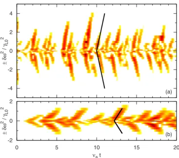
⬅k2共Q2+ P2兲, is used as a measure of the electric field am-plitude. These analytic expressions have been found to agree with 1D simulations of both ␦f and full-f BB model,25,26 with both Krook and diffusion-only collision operators, and with 3DHAGISsimulations.16Figure2共a兲shows the spectro-gram of a chirping solution in the aforementioned regime. In Sec. III, we consider frequency sweeping in a regime where ␦˙/
b
2⬇0.5, which approaches the limit of validity of the above theory.␦˙/b2 can be seen as a measure of the hole/ clump adiabaticity, and is roughly proportional to 共␥da兲1/2/␥L0 in the Krook case. When ␦˙/b
2⬇0.5, 4b/␦˙⬇2/b; in other words, a hole or a clump is
shifted by its width in a bounce time of deeply trapped par-ticles. In this regime, the previous analytic treatment is not relevant. However, numerical simulations show a similar square-root dependency of the frequency shift in time. We
-4 -2 0 2 4 ±δ ω 2 /γ L0 2 0 5 10 15 20 νat -2 0 2 ±δ ω 2 /γ L0 2 (a) (b)
FIG. 2. 共Color online兲 Spectrogram of the electric field, obtained with a moving Fourier window of size 510 for ␥L0= 0.1 and 共a兲 ␥d= 0.04,
␥da/␥L02 = 0.008, and= 1.0;共b兲␥d= 0.09,␥da/␥L02 = 0.043, and= 0.57.
Solid lines show the chirping velocity predicted by Eq.共9兲, with the correc-tion coefficient, and the chirping lifetime predicted by Eq.共12兲. Through-out this paper, the logarithmic color scale for each spectrogram spans three orders of magnitude.
introduce the effect of nonadiabaticity on chirping velocity as a correction parameter, defined as
⬅ ␦共t兲 ␣␥L0
冑
␥dt. 共11兲
is obtained numerically for␥L0/= 0.1 in Fig.3. We
con-firm that inside the validity limit of the above theory, ap-proaches unity. Even for relatively large values of ␦˙/b2,
the chirping velocity has a smooth dependency on the kinetic parameters. The latter point is crucial for the validity of the procedure described in Sec. III. The spectrograms corre-sponding to the two extreme points of Fig.3共a兲are shown in Fig.2.
The resonant velocity of a hole 共a clump兲 does not in-crease 共decrease兲 indefinitely. We define the lifetime of a chirping event as the time it takes to the corresponding power in the spectrogram to decay below a fraction e−2of the maximum amplitude reached during this chirping event. The maximum lifetimemaxis the maximum reached byduring a time-series, ignoring the first chirping event and any minor event. It is reasonable to assume that the island structure is dissipated by collisional processes, in which case the maxi-mum chirping lifetime should be of the form
max= a
a
, 共12兲
in the Krook case, and
max=d
␥L02
d3
, 共13兲
in the case with drag and diffusion when fⰆd, where a
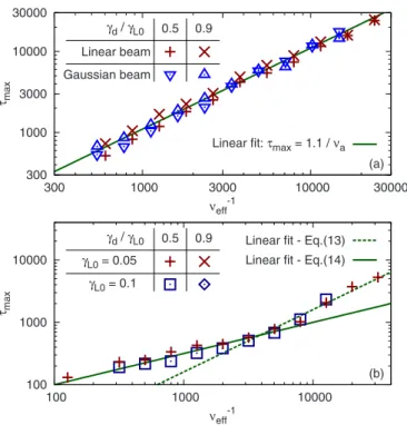
anddare constant parameters. In Fig. 4, we plot the
maxi-mum lifetime measured in COBBLES simulations where the ratio␥d/␥L0is chosen as 0.5 and 0.9, i.e., far from and close
to marginal stability, respectively. A quantitative agreement is found with Eq. 共12兲, with a= 1.1, for a−1 spanning two
orders of magnitude. With the diffusive collision operator, the chirping lifetime agrees with Eq.共13兲only for low col-lisionality. For high collisionality, diffusion affects the width of a hole or clump during the first phase of their evolution, namely, drive by free-energy extraction, which in turn affects
the decay by diffusion. Since chirping observed in experi-ments has a lifetime of the order of ⬃500, we adopt a semiempirical law obtained by a linear fit,
max=d
冉
␥L0 2 d 3冊
0.5 , 共14兲with d= 10. No repetitive chirping is found near marginal
stability for 0.05ⱕ␥L0ⱕ0.1, though longer computations may reveal this possibility.
In the following analysis of TAE experiments, Eqs.共12兲 and 共14兲 are used as diagnostics for the effective collision frequency; thus, it is important that these results are not too sensitive to the shape of the fast particles distribution. To investigate this point, we repeat the same analysis 共in the Krook case兲, this time with an initial bump-on-tail distribu-tion with a Gaussian beam instead of a constant gradient, or linear, beam. Figure4共a兲shows that the agreement is kept, even if the shape of the distribution has a significant effect on the extent of chirping as can be seen for example in Fig. 12 of Ref.26.
As long as the background plasma parameters are not significantly changed, chirping events in most tokamak ex-periments are quasiperiodic, with a quiescent phase between two chirping branches that lasts a few milliseconds. It should be noted that this statement does not seem to apply to DIII-D.20 In some parameter regimes, the chirping arising 0 0.2 0.4 0.6 0.8 1 0 0.02 0.04 β γdνeff/γL02 (a) Up-chirping Down-chirping 0 0.2 0.4 0.6 0.8 1 0.10-3 1.10-3 2.10-3 γdνeff/γL02 (b) Up-chirping Down-chirping
FIG. 3.共Color online兲 Correction to Eq.共9兲when the timescale of frequency shift is relatively short compared to the bounce period, for␥L0= 0.1. The
ratio␥d/effis such that␦共1/eff兲=0.2 in Eq.共9兲.共a兲 In the Krook case,
spectrograms for two extreme points are shown in Fig.2.共b兲 With drag and diffusion,d/f= 10. 300 3000 30000 1000 10000 300 1000 3000 10000 30000 τmax νeff-1 (a) Linear fit:τmax= 1.1 /νa Linear beam Gaussian beam γd/γL0 0.5 0.9 100 1000 10000 100 1000 10000 τmax νeff-1 (b) Linear fit - Eq.(13) Linear fit - Eq.(14) γL0= 0.05
γL0= 0.1
γd/γL0 0.5 0.9
FIG. 4. 共Color online兲 Maximum lifetime of a hole or clump, far from marginal stability,␥d/␥L0= 0.5, and near marginal stability,␥d/␥L0= 0.9.共a兲
With a Krook collision operator. The crosses correspond to the initial distri-bution shown in Fig.1共a兲, while the triangles correspond to a bump-on-tail distribution with a Gaussian beam. In both cases,␥L0= 0.05. The solid line
corresponds to Eq.共12兲.共b兲 With a diffusive collision operator 共for a linear distribution only兲 for two different values of linear drive. The dashed line corresponds to Eq.共13兲withd= 0.16, and the solid line corresponds to Eq.
共14兲withd= 10. The drag is chosen so that it does not significantly alter the
chirping lifetime,d/f= 10. An absence of points means that we do not
observe repetitive chirping before the end of the simulation共t=100 000兲.
from the BB model with Krook collisions is also quasiperi-odic, although the phase between two major chirping events is generally not as quiet as in the experiments. In a regime wherefⰆd, the chirping arising from the BB model with
drag and diffusive collisions is quasiperiodic too, but this time with clear quiescent phases in-between chirping events. In Fig. 1共b兲, which shows periodic decay and recovery of perturbation amplitude, corresponding to major chirping events, we observe qualitatively different behavior between the two collision models. In both case, no analytic theory has been developed to predict the average time between two chirping events,⌬tchirp. However, conceptually, there exists some relation with a subset of the input parameters. Thus, if we normalize time with the mode frequency, then chirping velocity, lifetime, and period are dictated by the input param-eters of the model,␥L0,␥d, anda, orfandd. In the Krook
case, we have a three-variable, three-equation system, which we solve by a fitting procedure described in Sec. III. With drag and diffusion, there is one additional degree of freedom; hence, the solution is not unique, but the boundaries of chirp-ing regime limit the possible range of input parameters.
III. ANALYSIS OF EXPERIMENTAL CHIRPING MODES
A. Fitting procedure
We consider magnetic field perturbations measured by a Mirnov coil at the edge of a fusion plasma, for a time inter-val during which quasiperiodic, perturbative chirping is ob-served, and during which background plasma parameters are not significantly changed, since a fixed mode structure is assumed to reduce the problem to a one dimensional Hamil-tonian. We also assume that frequency shifting occurs well within the gap of the Alfvén continuum, so that chirping lifetime is determined by collision processes, rather than by continuum damping. In the corresponding magnetic spectro-gram, we extract the linear mode frequency fA, the average chirping velocity d␦2/dt, the maximum chirping lifetime max, and the average chirping period ⌬tchirp. Equation 共9兲 gives a relation between linear drive and external damping,
␥L02 ␥d=
1 ␣22
d␦2
dt . 共15兲
With the Krook model, chirping is limited to a range where 0.2⬍␥d/␥L0⬍1.1.26 We found a similar constraint in our
simulations with drag and diffusion, although a full scan of parameter space remains to be done. From this observation, in both cases,␥L0is given within roughly 30% error, and␥d
within 50% error, by ␥L0⬇ 1.3
冉
1 ␣22 d␦2 dt冊
1/3 , 共16兲 ␥d⬇ 0.7冉
1 ␣22 d␦2 dt冊
1/3 . 共17兲We refine these estimations in a manner that depends on the collision model we adopt.
1. With Krook collisions
The analysis described here aims at estimating the values of␥L0,␥d, andafor which the␦f BB model fits
experimen-tal observations in terms of chirping characteristics. Equation
共12兲yields the effective collision frequency, a=
a
max
. 共18兲
Note that this effective collision frequency is meaningful only in the framework of a modelization by the simple Krook operator of all dissipative processes: particle colli-sions, particle source, and particle sink. Thus, this effective collision frequency a cannot be quantitatively compared
with experimental measurements of collision frequency un-less particle source and sink terms are fully identified as well. Equations共15兲and共18兲form a system of two equations with three unknowns. The remaining unknown is found by fitting the chirping period. In our simulations, the chirping period is estimated by searching for the dominant frequency in the Fourier spectrum of the electric field amplitude. To ensure a reasonable accuracy, simulations are performed for a time tⰇ⌬tchirp. If the experiment belongs to a regime where= 1, the above procedure is systematic. However, if is significantly smaller than unity, an iterative procedure is needed, with a feedback betweenand␥L02 ␥d.
2. With drag and diffusion
The analysis described here aims at estimating the values of␥L0,␥d,f, anddfor which the␦f BB model fits
experi-mental observations. Equations共14兲and共15兲form a system of two equations with four unknowns. The boundaries of the chirping regime yield an estimation ofdwithin 20% error,
d⬇ 1.2
冉
d max冊
2/3冉
1 ␣22 d␦2 dt冊
2/9 . 共19兲On the one hand, it is shown in Ref. 30 that for typical neutral beam-heated experiments, the ratio d/f is of the
order of unity. On the other hand, a numerical exploration of chirping regimes with drag and diffusion, which will be de-tailed in a future publication, suggests that whenfⱖd, the
drag significantly modifies the shape of chirping, to the point where we leave the regime of repetitive chirping. Thus, the relevant regime for friction isfⱗd. In this regime,⌬tchirp increases with decreasing f and ␥, and increasing d. To
refine the above estimations, and estimatef, we need a
two-dimensional scan in 共f,d兲, where we search for solutions
that fit the chirping period. In general,⫽1, and trial-and-errors are required to adjust the chirping velocity to the ex-perimental value.
B. Application to JT-60U
In JT-60U, TAEs are destabilized by a negative ion based neutral beam 共N-NB兲, which injects deuterons at Eb
= 360 keV. A distinction is made between so-called abrupt large-amplitude events共ALEs兲 and fast frequency sweeping 共fast-FS兲.32
In this paper, we focus on the latter phenomenon, which has a timescale of 1–5 ms, and with which the
asso-ciated redistribution of energetic ions is relatively small.33 ALEs are identified as energetic particle driven modes,34 have larger amplitude, shorter timescale共200–400 s兲, in-duce significant loss of energetic ions, and are out of the scope of this work since we assume a constant density of energetic ions.
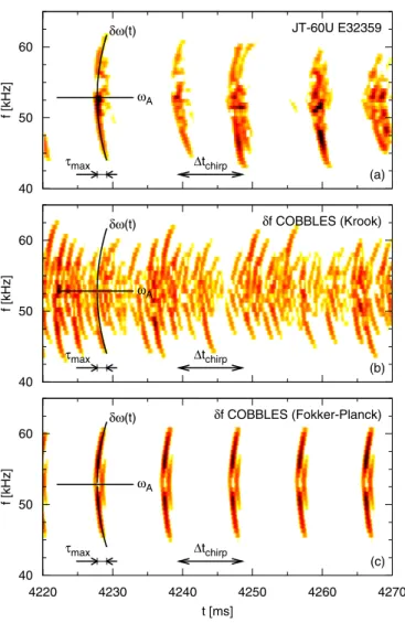
In the discharge E32359, around t = 4.2 s, frequency sweeping modes have been identified as m/n=2/1 and 3/1 TAEs.19 In the spectrogram shown in Fig.5共a兲, we measure fA= 53 kHz, d␦2/dt=6.3⫻10−5, max= 0.44⫻103, and ⌬tchirp= 3⫻103 共on average兲.
1. With Krook collisions
Equations 共15兲 and 共18兲 yield a= 0.25%, and ␥L0
冑
␥d= 1.8⫻10−2. However, the results of our analysis suggest that the plasma belongs to a regime where= 0.65, so we adjust the value of the product ␥L0
冑
␥d to 1.8⫻10−2/0.65=2.8⫻10−2.
A scan for this set of parameters is performed by chang-ing the slope of the distribution. Figure 6 shows that the chirping quasiperiod depends on␥Lin a roughly monotonous
way. Note that the scan needs to be performed on a relatively narrow range of the kinetic parameters, since the limits of subcritical regime and nonchirping共chaotic兲 regime yield a first estimate as ␥L⬃8%–12% and ␥d⬃4%–10%, in
per-centage of the mode frequencyA= 2fA. Here, the nonlin-ear stability threshold is defined as the largest value of␥Lfor
which the electric field amplitude tends to zero in the time-asymptotic limit, independently of the initial perturbation amplitude; the chaotic regime is defined and categorized in a way described in Ref. 26. We observe that the two-point correlation of electric field amplitude decreases as the system approaches marginality.
Figure5共b兲is the spectrogram for the simulation which is emphasized by a circle in Fig.6. The features of the main chirping events agree with the experimental observation. However, we observe a series of minor chirping events in between, which are absent from the experimental spectro-gram. Another caveat is that only symmetric chirping is ob-served with the ␦f BB model with Krook collisions and a linear velocity distribution. Thus, the application of this method with Krook collisions is restricted to symmetric or nearly-symmetric chirping experiments. The linear param-eters estimated from this analysis are shown in TableI. Our analysis suggests that the TAE in this discharge is marginally unstable, with␥/␥L⬃0.1, even though␥L⬍␥d, which is not
inconsistent with Eq.共5兲since␥L0⬎␥d. However, these
val-ues are inconsistent with estimations that take into account drag and diffusion processes. Since the following analysis
40 50 60 f [kHz] 40 50 60 f [kHz] 4220 4230 4240 4250 4260 4270 t [ms] 40 50 60 f [kHz] δω(t) ωA τmax Δtchirp δf COBBLES (Fokker-Planck) (c) δω(t) ωA τmax Δtchirp δf COBBLES (Krook) (b) δω(t) ωA τmax Δtchirp JT-60U E32359 (a)
FIG. 5. 共Color online兲 共a兲 Spectrogram of magnetic fluctuations during fast-FS modes in the JT-60U discharge E32359, obtained with a moving Fourier window of size 2 ms.关共b兲 and 共c兲兴 Spectrogram of the electric field where the kinetic parameters of the␦f BB model were chosen to fit the
magnetic spectrogram for JT-60U discharge E32359. The solid curve shows the analytic prediction for the chirping velocity.共b兲 Krook collisions, cor-rection parameter= 0.65. 共c兲 Friction-diffusion collisions, correction pa-rameter= 0.85. 0 2 4 6 8 10 8 8.1 8.2 8.3 8.4 8.5 8.6 8.7 Δ tchirp [10 3 ] γL[%] γ = 0 Stable JT-60U E32359 Supercritical simulation Subcritical simulation
FIG. 6. 共Color online兲 Scan of the chirping quasiperiod for the set of pa-rameters corresponding to JT-60U discharge E32359. The region where
␥/␥L⬎0.1, where ⌬tchirp⬍2⫻103is not included in this plot. Both linear
and nonlinear stability thresholds are indicated. The chirping quasiperiod agrees with the experiment for␥L⬇8.5%. The spectrogram for the circled
simulation is shown in Fig.5共b兲.
TABLE I. Frequencies and growth rates estimated from the magnetic spec-trogram of chirping TAEs, in percentage of the mode frequencyA= 2fA.
Collision model
␥L0
共%兲 共%兲␥L 共%兲␥d 共%兲a 共%兲f 共%兲d 共%兲␥
Krook 9.4 8.5 8.6 0.25 ¯ ¯ 0.7
Fokker–Planck 9.8 9.2 4.7 ¯ 0.36 1.7 4.6
shows much better agreement with the experiment, we imply that the Krook model is insufficient to describe nonlinear features related to repetition of chirping.
2. With drag and diffusion
We perform a first, rough scan in 共f,d兲 parameter
space, assuming= 1. Measuring average chirping velocity in repetitive chirping solutions yields an estimation of the correction parameter,= 0.85. Then Eqs.共16兲,共17兲, and共19兲 yield␥L0= 10⫾3%,␥d= 5⫾3%, andd= 1.7⫾0.4%. We perform
a second, more careful scan, which consists of a series of 4 ⫻8 simulations in the domain 共1.5%ⱕdⱕ2.2% and 1
ⱕd/fⱕ8兲, where␥L0and␥dare constrained by Eqs.共14兲
and 共15兲. The only repetitive chirping solution with 2500 ⬍⌬tchirp⬍3500 we found is shown in Fig. 5共c兲. We verify that chirping features measured in this simulation, d␦2/dt = 7.1⫻10−5 共6.2⫻10−5 for up-chirping and 7.9⫻10−5 for down-chirping兲,max= 0.45⫻103共0.47⫻103for up-chirping and 0.43⫻103for down-chirping兲, and ⌬t
chirp= 2.8⫻103, fit the experiment. The estimated linear parameters are shown in TableI. In theory, the solution is not unique, but the latter estimations are quite accurate because of the narrow range of periodic chirping regime. To validate this analysis, we com-pare the amplitude of perturbations in Fig. 7. Since the growth rate of chirping structure is neither␥ nor␥Land the
decay rate is not simply␥d but a function of several linear
parameters, the agreement we obtain is not trivial共we mea-sure a growth rate of 2.3% and a decay rate of 0.3%兲. For further validation, we estimate the values off andd from
plasma parameters in Sec. IV.
IV. ESTIMATION OF COLLISION FREQUENCIES A. Projection of Fokker–Planck collision operator
We consider collisions on energetic particles by thermal electrons共s=e兲, ions 共s=i兲, and carbon impurities 共s=c兲 and describe them by a Fokker–Planck collision operator35 that acts on the distribution f共x,v,t兲 of energetic particles 共s=b兲. In spherical coordinates 共v,⌰兲, neglecting gyroangle dependency,
冏
df dt冏
coll.=defl 1 2 1 sin⌰ ⌰冉
sin⌰ f ⌰冊
+ 1 v2 v冋
v 3冉
slowf + 1 2储v f v冊
册
, 共20兲 wheredefl,slow, and储are pitch-angle scattering,slowing-down, and parallel velocity diffusion rates, respectively, v储
⬅v·b=v cos ⌰ is the parallel velocity of energetic particles,
b⬅B0/B0, and B0 is the equilibrium magnetic field. We consider a TAE with toroidal mode number n, result-ing from the couplresult-ing of m and m + 1 poloidal modes. To simplify the following discussion, we consider strongly co-passing beam particles that resonate with the TAE at a ve-locityv⬇v储=vA, wherevA is the Alfvén velocity. Then, the
resonance condition is given by⍀=A, where ⍀ = nA v储 R0 − m v储 q共r兲R0 , 共21兲
R0is the major radius of the magnetic axis, q共r兲 is the safety factor, and r is the minor radius. To project the Fokker– Planck operator on the resonant surface, we follow the pro-cedure described in Refs. 11 and 30. We substitute vf by
Jb⍀f, where Pis the toroidal angular momentum, P⬅ −eb
c共r兲 + mbR0v储, 共22兲 J is the Jacobian of the coordinate transformation from v储to
⍀, J =P v储
冏
⍀ P冏v
储 =mcSmbv储 2r2ebB0 , 共23兲and S⬅rq
⬘
/q is the magnetic shear. Here, es and ms arecharge and mass of a species s, respectively, and b stands for beam particles. This procedure yields
冏
df dt冏
coll.=f 2f ⍀+d3 2f ⍀2, 共24兲 with f 2 =v储J共2储+slow−defl兲, 共25兲 d 3 =v 2 2J 2共储cos⌰ +deflsin⌰兲. 共26兲 We assume Maxwellian background distributions with same temperature T0. Typical experiments satisfy the follow-ing orderfollow-ing of thermal velocities:vTc⬍vTiⰆvAⰆvTe, while
the beam energy Eb is much larger than T0. With these as-sumptions, around the resonance,
10-4 10-3 10-2 10-1 4225 4227 4229 4231 Amplitude of perturbation (a.u.) t [ms] JT-60U E32359 Simulation
FIG. 7.共Color online兲 Evolution of the perturbation during a single chirping event. The signal is filtered between 40 and 65 kHz. In these arbitrary units, 10−3roughly corresponds to a noise level. The parameters of the simulation
are shown in TableI. For the simulation, to avoid hiding experimental data, we show the amplitude of perturbations instead of the perturbations them-selves. Note the use of arbitrary units 共we only compare normalized quantities兲.
f 2 =v储J v3
兺
s ns␥bs ms冋
erfs− 2s冑
e −s2册
, 共27兲 d 3 = J 2 2v3兺
s ns␥bs 2mbs 2再
关共2s 2− 1兲v ⬜ 2 + 2v 储 2兴erf s +2冑
s 共v 2− 3v 储 2兲e−s2冎
, 共28兲 wheres⬅v/vTs,v储=vA, ␥bs= 4eb 2 es 2 log⌳ mb , 共29兲and log⌳ is the Coulomb logarithm. Since the magnetic mo-ment is an invariant of the motion of injected beam ions from deposition to resonant surface,v⬜2=vb
2共1−R T 2/R 0 2兲, where v b
is the velocity of beam particles and RT is the tangential
radius of the beam. The equivalent collision operator in the Berk–Breizman model is obtained by substituting⍀=kv in Eq.共24兲.
B. Application to JT-60U
In the discharge E32359 around t = 4.2 s, the resonant surface of the m/n=2/1 and 3/1 TAE is located around r = 0.7 m. The magnetic shear is estimated from the q profile,36 S = 0.8. The deuteron plasma has the following characteristics: B0= 1.2 T, R0= 3.3 m, and the tangential ra-dius of the N-NB is RT= 2.6 m. At r = 0.7 m, ne= 1.4
⫻10−19 m−3, and T
0= 0.75 keV. We take into account car-bon impurities with Zeff= 2.7. With these equilibrium mea-surements, Eqs. 共27兲 and 共28兲 yield f/= 1.2% and d/
= 1.7%. Note that the electrons account for 99% off2, which reflects a high Alfvén velocity, while impurities account for 57% ofd3, which is consistent with the fact that pitch-angle scattering is more effective with heavier particles. The value ofdestimated in Sec. III B 2 quantitatively agrees with this
independent estimation. However, with our fitting procedure, f was underestimated by 70%. Though error bars in the
experimental data may account for this discrepancy, it is also possible that our model misses some mechanism that would enhance the friction.
V. CONCLUSION
In the present study, we found a regime of quasiperiodic chirping with both Krook and Fokker–Planck collision op-erators. Since quantitative agreement with theory suggests the predictability of nonlinear chirping characteristics based on fundamental linear kinetic parameters, the latter may be estimated in the opposite way from chirping data in experi-ments. More precisely, chirping velocity and lifetime yield two relations among␥L,␥d, and collision frequencies, and a
fitting of⌬tchirpyields an estimation of remaining unknowns. Note that major advantages of this technique are共1兲 kinetic parameters in the core of the plasma estimated only from the spectrogram of magnetic fluctuations measured at the edge, without expensive kinetic MHD calculations nor detailed core diagnostics, and 共2兲 unified treatments of supercritical
and subcritical AEs. We showed that drag and diffusion are essential to reproduce quiescent phases observed in experi-ments between chirping events. We confronted this proce-dure by analyzing AEs on JT-60U. We found quantitative agreement with measured magnetic fluctuations for the growth and decay of chirping structures and qualitative agreement with collision frequencies estimated from experi-mental background measurements. In these estimations, im-purities, which were not included in estimations of Ref.30, account for the main part of velocity diffusion. An effect of drag is to break the symmetry around the resonant velocity. The discrepancy between simulations and experiments in terms of asymmetry between up-shifting and down-shifting frequencies remains to be clarified. Preliminary results show that the shape of the energetic particle distribution has a sig-nificant effect on chirping asymmetry. In the present analy-sis, we chose a linear initial distribution. However, it is un-clear what shape of velocity distribution is relevant to the experiment. Many experiments in JT-60U and MAST feature repetitive chirping with velocity, lifetime, and period compa-rable to the TAE analyzed here, and we plan to apply the same procedure to these data in order to survey the depen-dency of kinetic parameters on fundamental plasma param-eters. Finally, we will work toward an analytic theory for the chirping quasiperiod, or an empirical formula, which would improve the robustness of our procedure.
ACKNOWLEDGMENTS
The main author expresses his thanks to Y. Todo, S. Pinches, and F. Zonca for crucial discussions about the ap-plicability of the BB model to fast-particle modes. This work was performed within the frame of a cothesis agreement be-tween the doctoral school of the Ecole Polytechnique, the Japan Atomic Energy Agency, and the Commissariat à l’Energie Atomique. It was supported by both the JAEA For-eign Researcher Inviting Program and the European Commu-nities under the contract of Association between EURATOM and CEA. Two of the authors, M.L. and Y.I. are supported by the MEXT under Grant No. 22866086. The views and opin-ions expressed herein do not necessarily reflect those of the European Commission. Computations were performed on Altix3700 and BX900 systems at JAEA.
1R. Aymar, V. Chuyanov, M. Huguet, Y. Shimomura, The ITER Joint
Cen-tral Team, and The ITER Home Teams,Nucl. Fusion 41, 1301共2001兲.
2C. Z. Cheng, L. Chen, and M. S. Chance,Ann. Phys. 161, 21共1985兲. 3A. Jaun, K. Appert, J. Vaclavik, and L. Villard,Comput. Phys. Commun.
92, 153共1995兲.
4A. Fukuyama and T. Akutsu, Proceedings of the 19th IAEA Fusion Energy Conference, Lyon, 2002共IAEA, Vienna, 2003兲, Vol. TH/P3-14, pp. 1–5. 5C. Z. Cheng,Phys. Rep. 211, 1共1992兲.
6D. Borba, H. L. Berk, B. N. Breizman, A. Fasoli, F. Nabais, S. D. Pinches,
S. E. Sharapov, D. Testa, and The EFDA-JET Workprogramme, Nucl.
Fusion 42, 1029共2002兲.
7J. Candy, D. Borba, H. L. Berk, G. T. A. Huysmans, and W. Kerner,Phys.
Plasmas 4, 2597共1997兲.
8S. D. Pinches, L. C. Appel, J. Candy, S. E. Sharapov, H. L. Berk, D.
Borba, B. N. Breizman, T. C. Hender, K. I. Hopcraft, G. T. A. Huysmans, and W. Kerner,Comput. Phys. Commun. 111, 133共1998兲.
9A. Fasoli, D. Borba, G. Bosia, D. J. Campbell, J. A. Dobbing, C.
Gorme-zano, J. Jacquinot, P. Lavanchy, J. B. Lister, P. Marmillod, J.-M. Moret, A. Santagiustina, and S. Sharapov,Phys. Rev. Lett. 75, 645共1995兲.
10A. Fasoli, D. Borba, B. Breizman, C. Gormezano, R. F. Heeter, A. Juan,
M. Mantsinen, S. Sharapov, and D. Testa,Phys. Plasmas 7, 1816共2000兲.
11H. L. Berk, B. N. Breizman, and M. S. Pekker, Plasma Phys. Rep. 23, 778
共1997兲.
12B. N. Breizman, H. L. Berk, M. S. Pekker, F. Porcelli, G. V. Stupakov, and
K. L. Wong,Phys. Plasmas 4, 1559共1997兲.
13H. V. Wong and H. L. Berk,Phys. Plasmas 5, 2781共1998兲.
14X. Garbet, G. Dif-Pradalier, C. Nguyen, P. Angelino, Y. Sarazin, V.
Grand-girard, P. Ghendrih, and A. Samain, in Proceedings of AIP Conference on
Theory of Fusion Plasmas, edited by O. Sauter, X. Garbet, and E. Sindoni
共AIP, Melville, NY, 2008兲, Vol. 1069, pp. 271–276.
15H. L. Berk, B. N. Breizman, and M. Pekker,Phys. Rev. Lett. 76, 1256
共1996兲.
16S. D. Pinches, H. L. Berk, M. P. Gryaznevich, S. E. Sharapov, and The
JET-EFDA Contributors,Plasma Phys. Controlled Fusion46, S47共2004兲.
17A. Fasoli, B. N. Breizman, D. Borba, R. F. Heeter, M. S. Pekker, and S. E.
Sharapov,Phys. Rev. Lett. 81, 5564共1998兲.
18R. F. Heeter, A. F. Fasoli, and S. E. Sharapov,Phys. Rev. Lett. 85, 3177
共2000兲.
19Y. Kusama, G. J. Kramer, H. Kimura, M. Saigusa, T. Ozeki, K. Tobita, T.
Oikawa, K. Shinohara, T. Kondoh, M. Moriyama, F. V. Tchernychev, M. Nemoto, A. Morioka, M. Iwase, N. Isei, T. Fujita, S. Takeji, M. Kuriyama, R. Nazikian, G. Y. Fu, K. W. Hill, and C. Z. Cheng,Nucl. Fusion39, 1837
共1999兲.
20W. W. Heidbrink,Plasma Phys. Controlled Fusion 37, 937共1995兲. 21K. G. McClements, M. P. Gryaznevich, S. E. Sharapov, R. J. Akers, L. C.
Appel, G. F. Counsell, C. M. Roach, and R. Majeski,Plasma Phys.
Con-trolled Fusion 41, 661共1999兲.
22E. D. Fredrickson, N. N. Gorelenkov, and H. L. Berk, Bull. Am. Phys.
Soc. 51共181兲, 181 共2006兲.
23M. Takechi, K. Toi, S. Takagi, G. Matsunaga, K. Ohkuni, S. Ohdachi, R.
Akiyama, D. S. Darrow, A. Fujisawa, M. Gotoh, H. Idei, H. Iguchi, M. Isobe, T. Kondo, M. Kojima, S. Kubo, S. Lee, T. Minami, S. Morita, K.
Matsuoka, S. Nishimura, S. Okamura, M. Osakabe, M. Sasao, M. Shimizu, C. Takahashi, K. Tanaka, and Y. Yoshimura,Phys. Rev. Lett. 83,
312共1999兲.
24M. Osakabe, S. Yamamoto, K. Toi, Y. Takeiri, S. Sakakibara, K. Nagaoka,
K. Tanaka, K. Narihara, and The LHD Experimental Group,Nucl. Fusion
46共10兲, S911 共2006兲.
25H. L. Berk, B. N. Breizman, and N. V. Petviashvili,Phys. Lett. A234, 213
共1997兲.
26M. Lesur, Y. Idomura, and X. Garbet,Phys. Plasmas 16, 092305共2009兲. 27B. Breizman, H. Berk, and H. Ye,Phys. Fluids B 5, 3217共1993兲. 28H. L. Berk, B. N. Breizman, and M. Pekker,Phys. Plasmas 2, 3007
共1995兲.
29P. Bhatnagar, E. Gross, and M. Krook,Phys. Rev. 94, 511共1954兲. 30M. K. Lilley, B. N. Breizman, and S. E. Sharapov,Phys. Rev. Lett. 102,
195003共2009兲.
31I. B. Bernstein, J. M. Greene, and M. D. Kruskal,Phys. Rev. 108, 546
共1957兲.
32K. Shinohara, Y. Kusama, M. Takechi, A. Morioka, M. Ishikawa, N.
Oyama, K. Tobita, T. Ozeki, S. Takeji, S. Moriyama, T. Fujita, T. Oikawa, T. Suzuki, T. Nishitani, T. Kondoh, S. Lee, M. Kuriyama, JT-60 Team, G. J. Kramer, N. N. Gorelenkov, R. Nazikian, C. Z. Cheng, G. Y. Fu, and A. Fukuyama,Nucl. Fusion 41, 603共2001兲.
33K. Shinohara, M. Takechi, M. Ishikawa, Y. Kusama, A. Morioka, N.
Oyama, K. Tobita, T. Ozeki, JT-60 Team, N. N. Gorelenkov, C. Z. Cheng, G. J. Kramer, and R. Nazikian,Nucl. Fusion 42, 942共2002兲.
34S. Briguglio, G. Fogaccia, G. Vlad, F. Zonca, K. Shinohara, M. Ishikawa,
and M. Takechi,Phys. Plasmas 14, 055904共2007兲.
35P. Helander and D. J. Sigmar, in Collisional Transport in Magnetized Plasmas, edited by P. Helander and D. J. Sigmar共Press Syndicate of the
University of Cambridge, Cambridge, 2002兲.
36N. Gorelenkov, S. Bernabei, C. Cheng, K. Hill, R. Nazikian, S. Kaye, Y.
Kusama, G. Kramer, K. Shinohara, T. Ozeki, and M. Gorelenkova,Nucl.