HAL Id: hal-03180347
https://hal.archives-ouvertes.fr/hal-03180347v2
Preprint submitted on 31 Mar 2021
HAL is a multi-disciplinary open access
archive for the deposit and dissemination of
sci-entific research documents, whether they are
pub-lished or not. The documents may come from
teaching and research institutions in France or
abroad, or from public or private research centers.
L’archive ouverte pluridisciplinaire HAL, est
destinée au dépôt et à la diffusion de documents
scientifiques de niveau recherche, publiés ou non,
émanant des établissements d’enseignement et de
recherche français ou étrangers, des laboratoires
publics ou privés.
Draw me Science - multi-level and multi-scale
reconstruction of knowledge dynamics with phylomemies
David Chavalarias, Quentin Lobbe, Alexandre Delanoë
To cite this version:
David Chavalarias, Quentin Lobbe, Alexandre Delanoë. Draw me Science - multi-level and multi-scale
reconstruction of knowledge dynamics with phylomemies. 2021. �hal-03180347v2�
Highlights
Draw me Science - multi-level and multi-scale reconstruction of knowledge dynamics with
phylomemies
David Chavalarias,Quentin Lobbé,Alexandre Delanoë
• we formalize the notion of level and scale of knowledge dynamics as complex systems,
• we propose a new class of meaning for the reconstruction of knowledge dynamics formalized by a new objective function parameterized by the level of observation,
• we properly formalize the concept of phylomemy as distinct from the concept of phylomemetic networks, • we propose a new reconstruction algorithm for phylomemetic networks reconstruction that outperforms previous
ones thanks to a new objective function,
• we show in case studies that this approach produces representations of knowledge dynamics close to the ones that can be obtained by synthesizing the points of view of experts on a given domain (glyphosate literature and knowledge and science mapping literature),
• we demonstrate with cases studies that this approach can be applied to any kind of unstructured corpora, even on relatively small data sets or short texts,
• we propose a new temporal clustering on dynamical graphs that is naturally part of the process of multi-level and multi-scale reconstruction of phylomemies,
• we integrate user preferences into our framework by providing an interaction model and contextualizing the different elements of our reconstruction workflow in the theoretical framework of the embodied cognition, • By applying our method to the state-of-the-art of this paper, we illustrate how it could be systematically applied
to generate such extended historical analysis which might be helpful to give more context to the scope and contributions of scientific papers.
Draw me Science - multi-level and multi-scale reconstruction of
knowledge dynamics with phylomemies
David
Chavalarias,
Quentin
Lobbé and
Alexandre
Delanoë
A R T I C L E I N F O Keywords:
phylomemy reconstruction knowledge dynamics
phenomenological reconstruction multi-scale and multi-level complex systems
science map co-word analysis
Abstract
The little prince asked Saint-Exupéry to draw him a sheep, but what if he had asked him to be drawn Science? How could he have done it and what could we have learned from it? In this article, we address the question of “drawing science” by taking advantage of the massive digitization of scientific production, and focusing on its body of knowledge. We demonstrate how we can reconstruct, from the massive digital traces of science, a reasonably precise and concise approximation of its dynamical structures that can be grasped by the human mind and explored interactively. For this purpose, we formalize the notion of level and scale of knowledge dynamics as complex systems and we introduce a new formal definition for phylomemetic networks as dynamical reconstruction of knowledge dynamics. We propose a new reconstruction algorithm for phylomemetic networks that outperforms previous ones and demonstrate how this approach also makes it possible to define a new temporal clustering on dynamical graphs. Finally, we show in case studies that this approach produces representations of knowledge dynamics close to the ones that can be obtained by synthesizing the points of view of experts on a given domain.
1
Introduction
1.1
The shapes of science
The little prince asked Saint-Exupéry to draw him a sheep, but what if he had asked him to be drawn Science? How could he have done it and what could we have learned from it?
Producing a global representation and understanding of the knowledge mankind has produced so far has been multi-century-old quest. In 1751, Jean le Rond d’Alembert, in his introduction of the first French Encyclopédie, stated his ambitions “to make a genealogical or encyclopedic tree which will gather the various branches of knowledge together under a single point of view and will serve to indicate their origin and their relationships to one another”1. Since then, several disciplines have investigated this question, from history and philosophy of science [17] to the emerging field of science mapping [21].
Science can be defined quite generically as “1) body of knowledge, 2) method, and 3) way of knowing” [1]. This body of knowledge is the result of the distributed interactions of thousands of scientists over the years; currently producing about two million documents per year - journal articles alone.
In this article, we will address the question of “drawing science” by taking advantage of the massive digitization of scientific production, and focusing on its body of knowledge. We demonstrate how we can reconstruct, from the massive digital traces of science, a reasonably precise and concise approximation of its structures that can be grasped by the human mind and explored interactively (an operation called phenomenological reconstruction2[4,17]). Science being a decentralized and dynamical process [36], complex systems methods are increasingly involved in the research domain of science of science (SoS) [74]. In this paper, we will model the semantic structures of science using
phy-lomemy reconstructiona method proposed by Chavalarias and Cointet [15] we are now extending to make it both more
1“former un Arbre généalogique ou encyclopédique qui les rassemble sous un même point de vûe, & qui serve à marquer leur origine & les liaisons qu’elles ont entre elles.”
2Phenomenological reconstruction is the process of choosing the appropriate data to be collected about phenomena and pre-structuring them to allow for a more comprehensive understanding in subsequent analyses. Ideally, phenomenological reconstruction may provide us with candidate concepts and relations, which, when integrated into modeling, can then serve as a basis for the human experimental work.
accurate and naturally multi-level and multi-scale. We will then demonstrate with some case studies how this achieves d’Alembert’s dream: of “[...] collecting knowledge into the smallest area possible and of placing the philosopher at a vantage point, so to speak, high above this vast labyrinth, whence he can [...] see at a glance the objects of their speculations and the operations which can be made on these objects; he can discern the general branches of human knowledge, the points that separate or unite them.”[31].
Finally, since the proposed methodology requires only time-stamped textual content, it can be applied to the re-construction of knowledge dynamics from any kind of corpora, which makes this approach very general and able to provide knowledge on any human activity, provided it leaves a digitalized written trace (e-mails, reports, patents, news, webpages, microblogs, etc.).
1.2
Levels and scales in complex systems
Complex systems display structures at all scales with a hierarchical organization reflecting the interactions between the entangled processes that sustain them [13]. Their description mobilizes the notions of ‘levels’ and ‘scales’, “level being generally defined as a domain higher than ‘scale”’ and ‘scale’ referring to the structural organization within a level [41]. In biology for example, the choice of level of observation determines what the main entities under study (individuals, organs, cells, genes, etc.) are, while the choice of a scale determines the smallest resolution adopted to describe these entities.
The method presented in this paper makes a clear distinction between these notions of level and scale in the phe-nomenological reconstruction of knowledge dynamics3, a distinction that is not made explicit by other scholars or science modeling approaches. The choice of a level of observation determines the range of intrinsic complexity of the dynamic entities we want to observe, the choice of a scale defines the extrinsic complexity of their description4. One of the main difference between level and scale is that the concept of level is ontologically linked to the notion of time since the components of a level derive their unity from some underlying dynamic process ; while the notion of scale does not necessarily imply time.
1.3
Levels of observation of Science
At a given level of observation, science is composed of different research domains whose unity over time is charac-terized by core questions and research objects. For example, at a very high level, one may find social sciences, biology,
physics, etc.; at a lower level, one will find sociology, cell biology, quantum mechanics ; and at an even lower level,
political sociology, proteomics or quantum cryptography.
Levels are sustained by socio-economic processes that guide the progress of science with more or less of a broad focus (laboratories, national and international research networks, national and international funding schemes, journals, etc.). Their sub-components are evolving socio-semantic macro-structures that are reflected by the specialization of certain journals, conferences or the presence of sub-categories in digital archives.
In this article, we will propose a definition of what the components of a level of organization of Science are. We will call these components branch of science. We will also detail a method to identify and represent them.
2
Related work
2.1
Mapping science and knowledge
Producing science maps and knowledge maps, as our in-depth analysis of 14k papers will show (see SIAppendix B
and SI Fig. 2 and 3), has been addressed by two scientific approaches, each of them having known recent developments regarding evolution, dynamics and temporality.
1. Bibliometrics is defined as the use of statistical methods to analyze digitized textual corpora. The part of this domain dealing with science mapping is divided into two major components:
• Citation and co-citation analysis (CA) emerged in the 1970s [33] with the aim of measuring and analyzing scholarly literature. Primarily focused on the assessment of scientific output, it quickly diversified with the analysis of large citation landscapes through methods such as co-citation and bibliographic coupling [39,56]. Later on, following the creation of the Web, these methods were generalized as part of the study 3Note that some scholars use the term ‘resolution’, ‘zoom’ or ‘granularity’ instead of ‘scale’.
4Are we only interested in the main concepts of the fields or in a finer granularity of a myriad of terms? Do the details of the interactions between terms matter? Does the scientific field under study evolve linearly or with ramifications? etc.
of hyperlinked data [40]. Methods to describe conceptual structures of science such as research fronts, hot
topicsand trends, etc. [71,9] came at the forefront of this research domain. Over the last decade, a growing
number of contributions have proposed temporal reconstructions of the citation landscape [20,23,12]. • Co-word analysis (CWA) is a bottom-up approach first developed by sociologists in the 1980s [11] to
reconstruct the dynamics of research themes out of words co-occurrence. It has developed in the last decade into a generic approach to map knowledge dynamics in unstructured corpora [15,68,52]. Citation and co-word analysis research areas share common objectives, namely to understand the structures of science. This is reflected by their proximity on the map of SI Fig. 2. They form a toolkit that is at the core of the bibliometrics approach to science of science. Their parallel development has quickly paved the way to hybrid research between co-word and citation analysis [6,5] or social and semantic networks [51]. Finally, the growth of scientific databases has stimulated the visualization of wide citation landscapes [57] or complex atlases of sciences [7,8].
2. Information retrieval (IR) deals with the retrieval and evaluation of information from digitized document repositories. It has mobilized latent semantic analysis and topic modeling in the early 2000s at the instigation of a community of statisticians who introduced the latent dirichlet allocation method [3]. The general context was the characterization of a collections of documents, one of the aim being to be able to structure the result of a query with a “bottom-up” approach. The use of topic modeling mostly focuses on document classification [70], recommendation [67] or sentiment analysis [43]. Some scholars also proposed methods to organize a set of retrieved documents according to their topics and temporal relationships [42,53]. More recent works started to tackle the mapping of scientific issues and their dynamics at the scale of a research area [46,35,26,54,73,38]. More recently, the idea of working on latent semantic spaces has been taken up by the research field of machine learning with approaches such as words embedding [63,61]. It has been mostly used for the purpose of information retrieval and documents classification (which is the reason why it appears in the same group as LDA in the SI Fig. 2), but can also be a useful tool to analyze science’s evolution, mostly at the micro-level of terms-to-terms similarities [49,63,61].
2.2
Mapping knowledge dynamics
Our methodology belongs to the science of science, whose first objective is the reconstruction of scientific land-scapes and their dynamics. In order to highlight the advantages and disadvantages of the methods issued from the various approaches we have just described, we have identified their key properties in SI sectionB.2.
We have used these criteria inTable 1and ??, to compare some key papers from each methodological approach. Our approach meets all of them contrary to most previous studies. Among others, none of them really formalize the distinction between the notions of ‘level’ and ‘scale’.
2.3
Phenomenological reconstruction of science with phylomemies
To observe and further understand through modeling a complex object 𝑂 ∈ , we first select the properties to be observed and measured, then reconstruct from the data collected those properties and their relations as a formal object
𝑅∈ described in a high-dimensional space. Then some dimension reduction is applied to 𝑅 to get a human-readable representation in a space . The chain ⟼ ⟼ defines what is called phenomenological reconstruction [4,17]. The quality of a phenomenological reconstruction is measured by its ability to propose, from the raw data, representations in that make sense to us and provide affordances for modeling and conceptual understanding5.
Phylomemy reconstruction is a general methodology for the processing of unstructured and dynamical textual corpora that is part of the co-word analysis framework[10]. It can be applied to any kind of corpora, from scientific papers [15,16] to news papers [18] or political discourses [52], in order to identify the topics they cover and the dynamical structures generated by the development of these topics.
In this paper, we will define formally a category of meanings conveyed by phylomemies [15] as phenomenological reconstructions. We will then show how this definition can be made operational and allow users to naturally grasp the multi-level and multi-scale structure of knowledge dynamics through the definition of 1) ⟼ , the operator that reconstructs a multi-level and multi-scale structure, and 2) ⟼ , projector that selects a level of observation and 5Even though hypotheses about the underlying processes that have generated the data could help to find the relevant phenomenological recon-struction method, a phenomenological reconrecon-struction does not make such hypotheses.
Table 1
Comparison between different approaches for the modeling of knowledge dynamics. The column ‘meaning’ indicates
whether the approach can distinguish between paradigmatic (P) and syntagmatic (M) relations among terms, process both
or one in particular, or cannot make this distinction at all. Symbol means that the feature is not part of the study or not
compatible with the approach. Abbreviations. Domains of origin: Science of Science (SoS), Information Retrieval (IR), Machine Learning (ML), Visual Analytics (VA) ; Method: Complex Network Analysis (CNA), Co-Word Analysis (CWA), Word Embedding (WE), Topic Modeling (TM), Citation Analysis (CA)
Paper Domain Focus Unit of analysis Methods Fields detection Meaning
This paper SoS corpora based text CWA COC P+S
[52] SoS corpora based text CWA COC P+S
[68] SoS corpora based text CWA COC P+S
[15] SoS corpora based text CWA COC P+S
[54] IR corpora based text CWA COC P+S
[42] IR corpora based documents CNA MGF
[61] ML corpora based codes WE P
[49] ML corpora based codes WE P
[38] IR corpora based documents TM DTM (LDA) P
[19] IR corpora based documents TM LDA P
[73] Visual analytics corpora based documents TM HLMT
[66] IR corpora based documents TM dDTM
-[26] IR corpora based documents TM HDP
[35] IR/ML corpora based documents TM PLSA
[12] SoS corpora based documents CA BC
[23] SoS corpora based documents CA BC S
[37] SoS query based documents TM + CA PLS + CA [53] IR query based documents IR
propose to explore this level in a multi-scale way. At the same time, we make tangible the different shapes generated by science, which can be visualized with an appropriate free software (cf. [44]). More discussions on the relations between the phenomenological reconstruction of science with phylomemies, formal modeling and history and philosophy of science can be found in [17].
3
Materials and methods
3.1
Generic workflow of phylomemy reconstruction
1. Indexation 2. Similarity measure 3. Fields detection (clustering) 4. Inter-temporal matching
Figure 1: Workflow of phylomemy reconstruction from raw data (digitized textual corpora) to global patterns. The output
is a set of phylomemetic branches where each node is constituted by a network of terms describing a research field. These nodes are a proxy of scientific fields and can have different statuses: emergent, branching, merging, declining. Source: [15]
The workflow of phylomemy reconstruction (cf. Figure 1and [15]) takes as input a large set of documents produced over a period of time (the raw data in ), and provides as output a structure that characterizes, at a given spatio-temporal resolution, the transformations of the knowledge domains covered by . An example of such output can be seen in the phylomemy of glyphosate-related academic literature (Figure 2) and is detailed as a case study in SI sectionF.
The workflow for phylomemy reconstruction uses advanced text-mining and complex networks analysis. It can be roughly decomposed into four operators Φ =4Φ◦3Φ◦2Φ◦1Φthat correspond to four main steps (seeFigure 1):
Figure 2: The visualization of the phylomemy 𝑔𝑙𝑦𝑝ℎ𝑜𝑠𝑎𝑡𝑒 (16,655 documents) at the level 𝜆 = 0.8 between 1995 and 2020
with branches smaller than 3 filtered out. Each connected dot represents a specific field of research described by several
key-words (as displayed for example in the magnified area: {glyphosate, herbicides,antioxidative enzyme,oxidative stress,
superoxide dismutase,reactive oxygen species}). Emerging terms are highlighted in red in the description of the field and are displayed in large fonts on this figure, close to the earliest fields that mention them. Inter-temporal matching between fields is represented by vertical links and a group of connected fields defines a branch of science. The branch highlighted by a dotted box starts in 2006 and deals with majors negative side-effects of glyphosate-based products. It was indeed in the 2000s that significant discrepancies were documented regarding the decomposition and residues of glyphosate, between laboratory experiments on glyphosate and field experiments on glyphosate-based products, raising concerns about their
effects on health and on the environment. Details about this case study are given in SI section F. An interactive version
of this visualization, available online at http://unpublished.iscpif.org/glyphosate, can be downloaded from the
archives [59] (data), [58] (explorer). See [44] for details.
1Φ. Indexation. The core vocabulary of is extracted as a list = {𝑟
𝑖 |𝑖 ∈ }, where 𝑟𝑖 are groups of terms (thereafter called roots) conveying the same meaning according to the analyst6. An ordered series ∗ = {𝑇𝑖}1≤𝑖≤𝐾, 𝑇𝑖 ⊂ , of sub-periods of is defined to determine the temporal resolution of the reconstruction. Co-occurrences of roots within the documents are then processed per period of time.
2Φ. Similarity measures. Each period-dependent, root co-occurrence matrix is transformed into a root-to-root similarity matrix after the appropriate similarity measure has been chosen. This choice should be oriented by the research question at stake, as described for example in [28] or [69]. Depending on the question, two reconstructions using two distinct classes of similarity measures may prove complementary (see also SI.B). 3Φ. Fields detection and clustering. Within each period, the completion of2Φ◦1Φresults in temporal series of
networks of roots similarities. A community detection algorithm7is then applied to identify, within these net-works and for each period of time 𝑇𝑖 ⊂ , important sub-units constituting “fields of knowledge”, i.e. dense networks of multi-terms characterizing key research questions. Research on community detection algorithms has been very prolific [32] and several algorithms with different intrinsic spatial resolution could potentially be 6These groups could be obvious e.g. {decision-making processes, decision making process, decision making processes} or more customized to the analyst’s point of view, e.g. {advertising, advertisement, advertisements, advertiser}.
suitable at this step. The result of fields detection is a temporal series of clusters of roots 𝐶𝑗 computed over ∗: ∗ = {𝑇|𝑇 ∈ ∗}where 𝑇 = {𝐶
𝑗|𝑗 ∈ 𝐽𝑇,}and 𝐶𝑗 = {𝑟𝑖 |𝑟𝑖 ∈ , 𝑖 ∈ 𝑗 ⊂ }. We will note =⋃𝑇∈∗𝑇 the set of all clusters over all periods.
4Φ. Inter-temporal matching. Once the fields of knowledge have been identified as a temporal series of clusters, inter-temporal matching reconstructs the lineage between these clusters. This inter-temporal matching operation brings time into play. Consequently, this is where the notion of level arises. The result of4Φis an evolving structure describing the evolution of large knowledge domains and it has been called a phylomemetic network [15].
Steps 1 to 3 are very common steps in science and knowledge mapping literature in which, at each stage, several options are available to the modeler according to his/her initial research questions8. In the following sections, we will focus on4Φand how it can convey the notions of level and scale, setting arbitrary parameters for1Φto3Φ. The reader interested in these particular steps can find more examples and technical details in [15,24,14,27].
3.2
Method of reconstruction of the dynamics
The most general assumption on the evolution of fields of knowledge, subsequently defined has roots clusters, is that some are likely to emerge, split, merge or die (see [48] for pioneer work or [50] for a review). The problem can be formulated as follows: find, for any cluster 𝐶𝑇 at period 𝑇 , the combination of clusters from previous periods, if any, that could best account for the presence of 𝐶𝑇 at 𝑇 (the ‘parents’ of 𝐶𝑇), as well as the set of clusters from subsequent periods that could be the continuation of cluster 𝐶𝑇 (the children of 𝐶𝑇). This is achieved through the definition of some parentage metrics and the selection of the most relevant ‘parents’ and ‘sons’ for each cluster, when they exist.
Once chosen a parentage metrics, computing the weighted inter-temporal associations between clusters is the easy part. The hard part is to choose the one to keep.
First, since filtering out some inter-temporal associations has a direct impact on the overall connectivity of the dynamic structure, and consequently on the number of sub-components, the interpretation of the final result depends strongly on the pruning procedure.
Second, since the goal is to highlight the continuities in the evolution of clusters, parents and children of a particular cluster will be looked for as close in time as possible. The trade-off between association strength and highlight of continuities in evolution is not straightforward. When allowing matching between non-consecutive periods, this trade-off directly influences the average time difference between related fields and the global understanding of the final output.
As we will see, this entanglement between the granularity of the macro-structures revealed by a temporal recon-struction and the timescale of inter-temporal matching is where the multi-level aspect of phylomemy comes into play.
3.2.1 Upstream and downstream inter-temporal matching
An up-stream inter-temporal matching function is based on a similarity measure Δ ∶ × () → [0, 1] that defines the ‘strength of association’ between any clusters 𝐶𝑇 ∈ and any set of clusters {𝐶
𝑗}𝑗 ⊂ () belonging to strict anterior periods 𝑇′(noted 𝑇′ ≺≺ 𝑇)9. Starting from a cluster similarity function Δ, Chavalarias and Cointet [15] proposed to find for every period 𝑇 ∈ ∗, for every cluster 𝐶𝑇 computed over the period 𝑇 and for every threshold
𝛿≥ 0 the closest satisfactory set of ‘parents’4Φ≺ 𝛿(𝐶
𝑇)according to Δ with their association strength: 4 Φ≺𝛿(𝐶𝑇) = ({𝐶𝑗 ∈ 𝜅𝐶≺𝑇}, 𝑤) Where: • 𝜅≺ 𝐶𝑇 = arg 𝑚𝑎𝑥Δ(𝐶𝑇,𝜅)[ arg 𝑚𝑖𝑛{𝜏(𝐶𝑇,𝜅)|𝜅⊂𝑇 ′≺≺𝑇,Δ(𝐶𝑇,𝜅)≥𝛿}𝜅], • 𝑇′≺≺𝑇
= {𝐶𝑇′∈|𝑇′≺≺ 𝑇}is the set of all clusters of whose period is strictly anterior to 𝑇 ,
8For example, step 1.2 can proceed from advanced text-mining on the corpora, or be made via external ontologies or thesaurus (e.g. PubMed Mesh).
• 𝜏(𝐶𝑇, 𝜅)is the minimum amount of time elapsed between the period 𝑇 and the periods of the clusters constituting
𝜅10.
• 𝑤 = Δ(𝐶𝑇, 𝜅≺
𝐶𝑇
)
∈ [0, 1]is the association strength between 𝐶𝑇 and its “parents”.
As the definitions of parents and children of a cluster are symmetrical with respect to time, inter-temporal match-ing is consequently symmetrized by considermatch-ing both the up-stream4Φ≺
𝛿(𝐶
𝑇)and the symmetric down-stream inter-temporal matching function4Φ≻
𝛿(𝐶𝑇), where the association strength between any clusters 𝐶𝑇 ∈ and any set of clusters {𝐶𝑗}𝑗 ⊂() belonging to strict posterior period 𝑇′′(noted 𝑇′′≻≻ 𝑇) is also processed (see SIC.4for full description).
We thus define4Φ ∶ × [0, 1] ⟼ ((), 𝑤)2defined as11:4Φ
𝛿(𝐶) = ((4Φ ≺ 𝛿(𝐶),
4Φ≻ 𝛿(𝐶))
3.2.2 Phylomemies as foliation on temporal series of clustering
Thereafter, we will work with the following definitions:
Definition: Temporal series of clustering∗.Let ∗be an ordered set and = {𝑟
𝑖|𝑖 ∈ } be a set of elements. A temporal series of clustering over is defined as ∗= {𝑇|𝑇 ∈ ∗}where 𝑇 = {𝐶𝑇
𝑗 |𝐶 𝑇
𝑗 ⊂()}𝑗∈𝐽𝑇.
Definition: Foliation on a temporal series of clustering(cf. Figure 3). Let ∗ = {𝑇|𝑇 ∈ ∗}be a temporal series of clustering and =⋃𝑇∈∗𝑇, a foliation on ∗is defined as a function Φ ∶∶ × [0, 1] ⟼ (() × [0, 1])2 such as:
1. ∀𝐶 ∈ 𝑇,∀𝛿 ∈ [0, 1], Φ(𝐶, 𝛿)(1, 1) ⊂(𝑇′≺≺𝑇)(parents of 𝑇 at 𝛿, associated with strength Φ(𝐶, 𝛿)(1, 2)), 2. ∀𝐶 ∈ 𝑇,∀𝛿 ∈ [0, 1], Φ(𝐶, 𝛿)(2, 1) ⊂(𝑇′≻≻𝑇
)(children of 𝑇 at 𝛿, associated with strength Φ(𝐶, 𝛿)(2, 2)),
Definition: Phylomemy. A phylomemy 𝜙 is a foliation on a temporal series of clustering ∗. It describes, for any cluster 𝐶𝑇
𝑗 in temporal components of
∗and any threshold 𝛿, the relevant inheritance linkages of 𝐶𝑇
𝑗 . Consequently, for the study of knowledge dynamics, is the space of all foliations on temporal series of roots clustering.
Definition: Weighted inheritance networks. Let ∗ = {𝑇|𝑇 ∈ ∗} be a temporal series of clustering. A weighted inheritance network 𝜑 ∶ ⟼ (() × [0, 1])2is a function defined over the set of nodes =⋃
𝑇∈∗𝑇 such as ∀𝐶𝑇 𝑗 ∈; 𝜑(𝐶 𝑇 𝑗 )(1, 1) ⊂( 𝑇′≺≺𝑇 )and 𝜑(𝐶𝑗𝑇)(2, 1) ⊂(𝑇′≻≻𝑇 )12.
Definition: Phylomemetic network. Let 𝜙 be a phylomemy over ∗ and Π ∶ ⟼ [0, 1], a phylomemetic
networkis defined by 𝜑Π= {(𝐶𝑗𝑇,4Φ≺Π(𝐶𝑇
𝑗)(𝐶
𝑇 𝑗))|𝐶
𝑇
𝑗 ∈}. It is a plaque of the phylomemy 𝜙 that defines a weighted inheritance networks over a temporal series of root clusters. It is thereafter possible to visualize the inheritance patterns of 𝜑Πin in order to understand the structure of 𝜙 (cf.Figure 2and [44]).
is consequently the space of all weighted inheritance networks of root clusters, and phylomemetic networks are elements of that can be defined as a plaque of a particular phylomemy.
10Their approach makes it possible to have several sets of parents for a given cluster although this situation is quite rare. Also, since a given cluster could be in the set of parents of several subsequent clusters, a cluster might have many children.
11It is worth mentioning that this function looks for the first correspondence that, from a temporal point of view, satisfies a given threshold 𝛿, instead of looking for all potential correspondences for all time and taking the optimum - an approach adopted among all the works referenced in
??that are going beyond the simple correspondence between consecutive periods.
12We note 𝜑(𝐶𝑇)(1, 1)the first component of the first tuple of 𝜑(𝐶𝑇) = ((, 𝑤
1), (, 𝑤2)), i.e. , and 𝜑(𝐶𝑇)(2, 1)the first component of the second tuple, i.e. .
Figure 3: Local structure of a foliation on a temporal series of clustering ∗parameterized by 𝛿. Locally, above the cluster
𝐴 ∈ 𝑇 ⊂ ∗ from period 𝑇 , 𝛿 parameterized the different sets of parents and children of 𝐴 for different satisfaction
threshold in inter-temporal matching. As we raise 𝛿, the parents and children of 𝐴 might change. At 𝛿0, clusters 𝐵 and
𝐶 ∈𝑇−1 are the parents of 𝐴 ; but when we raise 𝛿 to 𝛿
1, the pair {𝐵, 𝐶} of parents is no longer valid for 𝐴 and the
cluster 𝐹 from a former period 𝑇 − 2 has to be mobilized to describe the lineage of 𝐴 as the child of {F}. Eventually, some branches might split or merge due to these reconfigurations (e.g. here the segment starting from 𝐸 becomes the
starting of a new branch at 𝛿2). A phylomemy is a foliation over a temporal series of clustering ∗.
3.2.3 Quality assessment of phylomemetic networks and levels of observation
To assess the quality of a phenomenological reconstruction, [22] make the distinction between “interpretation as the facility with which an analyst makes inferences about the underlying data and trust as the actual and perceived accuracy of an analyst’s inferences.”
Reconstructions of knowledge dynamics, regardless of the methodology (cf.section 2), generally offer rich oppor-tunities for interpretation because one naturally interprets salient events in the reconstruction (e.g. split, emergence, etc. of fields/clusters) as related to the fate of scientific fields. This richness of interpretability is however rarely backed with a high level of trust. The distinction between phylomemies belonging to and phylomemetic lattices that belongs to gives more theoretical grounding to the assessment of trust of phenomenological reconstruction.
In the framework of this generalization, [15] appear to have studied the specific case where the operators ⟼ are all uniform projectors Π = 𝛿, i.e. 𝜑𝛿 = {(𝐶𝑗𝑇,
4Φ≺
𝛿(𝐶𝑗𝑇))|𝐶 𝑇
𝑗 ∈}. The results obtained so far by [15] show that, for a wide range of 𝛿 values, there are robust correlations between the structural properties of fields assessed at specific period 𝑇 , and their dynamical properties inferred from their position in the branches of 𝜑𝛿 (i.e. emergent, declining, etc. seeFigure 2). This observation means that we can trust the interpretation our common sense associates to the fact that a field occupies some salient position in a phylomemy.
There is no reason to think however that a uniform projector Π𝛿 will provide the same level of description for all knowledge domains. Moreover, since no objective function has been proposed to help the analyst interpret and choose the value of 𝛿, there are some concerns about the actual as opposed to perceived accuracy of inferences one can make when comparing branches of a phylomemy or interpreting their distribution.
To get around this problem, we propose a class of meanings for the operation ⟼ that is commonly under-standable. In order to do so, let’s come back to D’Alembert’s dream to “distinguish the general branches of human knowledge” and let’s imagine D’Alembert asking someone (𝑥) ∶ “draw me a branch of knowledge that deals with
𝑥”, the same way we could have asked him: “give me a chapter of the Encyclopedia that deals with 𝑥”.
If we have at our disposal a phylomemy of science 𝜙 ∈ over the temporal series of clustering ∗of roots , for all 𝑥 in , we can draw inspiration from information retrieval to shape an answer to (𝑥).
An answer to D’Alembert’s question could consist in pointing to a given phylomemetic branch 𝐵𝑘⊂ 𝜑containing some elements of 𝑥: “here is the temporal description of a domain of research concerned by 𝑥” ; where :
• 𝜑 =⋃𝑘𝐵𝑘∈ is a representation of a phylomemy 𝜙, • 𝑥is the set of all fields containing 𝑥,
• 𝑥are the periods covered by 𝑥,
Let’s note 𝐵𝑘the set of all the fields of the branch 𝐵𝑘, we propose two metrics to assess the relevance of 𝐵𝑘to (𝑥):
• The precision 𝜉𝑘 𝑥=
|𝑥∩𝐵𝑘|𝑥|
|𝐵𝑘| of 𝐵𝑘against 𝑥. It is related to the probability to observe 𝑥 by choosing at random
a cluster in 𝐵𝑘within 𝑥, • The recall 𝜌𝑘
𝑥 =
|𝑥∩𝐵𝑘|
|𝑥| of 𝐵𝑘against 𝑥. It is related to the probability to be in 𝐵𝑘when choosing a cluster
about 𝑥 at random in 𝜙.
An answer 𝐵𝑘to (𝑥) will be all the more precise regarding 𝑥 that its precision 𝜉𝑥𝑘is high. But it will provide all the more information about the different historical contexts of 𝑥 that its recall is high. Precision and recall are generally antagonistic and consequently, the questioner has to indicate the desired ‘trade-off’ in his/her question.
The quality of an answer (𝑥) can be assessed with respect to the desired level of trade-off 𝜆 ∈ [0 1] between precision and recall with the following 𝐹 -score function:
𝐹𝜆(𝑥, 𝑘) =(1 + 𝑓 (𝜆) 2).(𝜉𝑘 𝑥.𝜌 𝑘 𝑥) 𝜌𝑘 𝑥+ 𝑓 (𝜆)2.𝜉𝑥𝑘 where 𝑓(𝜆) = 𝑡𝑎𝑛(𝜋.𝜆
2 ). For 𝜆 = 0, only the precision counts, whereas for 𝜆 = 1, only the recall counts13.
Several branches could mention 𝑥, which means that we also have to know which 𝐵𝑘to propose first as an answer. For this reason, we introduce a generic choice function Ψ (a random variable to be determined later) that tells which branch among the branches containing 𝑥 will be the first to be examined by D’Alembert.
The objective function for the evaluation of the relevance of 𝜙 in answering (𝑥) thus becomes:
𝐹𝜆𝑥(𝜑) = Σ𝐵
𝑘∈𝜑|𝐵𝑘∩𝑥≠∅Ψ𝑥(𝑘).𝐹𝜆(𝑥, 𝑘) (1)
If we wanted to provide D’Alembert with independent answers for every 𝑥, we could search, for each question (𝑥), the phylomemetic network with the best 𝐹𝑥
𝜆 score. However, this would prevent D’Alembert from having a global vision of science and of the articulation between its different branches: answers based on different queries will indeed not necessarily be comparable.
In order to provide a global representation 𝜑 of a domain of science, we thus have to assess the relevance of a particular phylomemetic network for its ability to answer any question (𝑥) D’Alembert might ask about elements of . Since some 𝑥 may interest D’Alembert more than others, the optimal 𝜑 should take into account the interest profile of D’Alembert for elements of . We will call Ξ the choice function over that determines the probability of D’Alembert asking for a particular 𝑥.
Given the choice functions Ξ and Ψ, the global 𝐹 -score of a representation 𝜑 of a phylomemy can be defined as:
𝐹𝜆(𝜑) = Σ𝑥∈Ξ(𝑥).𝐹𝜆𝑥(𝜑) (2)
Note that Ξ is a property of the questioner whereas Ψ can be a property of either the respondent or the questioner. Ξand Ψ are both random variables on which the meaning of a given phylomemy projection 𝜑 will depend. We will see insection 6how these two functions can be determined empirically.
Branches with high recall for a given 𝑥 will tend to be more complex to interpret because the contexts in which 𝑥 is set are very varied and provide a huge amount of information, whereas branches with high precision for a given 𝑥 will tend to be simpler because they target very homogeneous contexts.
Consequently, 𝐹𝜆is a score of quality whose parameter 𝜆 can be related to a desired level of observation. For high
𝜆values, the phylomemies with the highest 𝐹𝜆score will be the ones that include large complex branches whereas for
low 𝜆 values, phylomemies with small homogeneous branches will score the highest.
The objective function 𝐹𝜆 gives meaning to the problem of choosing a projector ⟼ : given a level of
observation of a phylomemy 𝜙, what is the best projector to optimize the information conveyed by the corresponding
phylomemetic network?The next section proposes an approach to solve this problem.
13We consider for 𝐹
3.2.4 Adaptive inter-temporal matching and step phylomemetic networks
Let’s consider a reconstruction operator4Φ ∶ × [0, 1] ⟼ ((), 𝑤)2that from a partial phylomemy reconstruc-tion workflow (steps 1 to 3), reconstructs the inter-temporal matching links from a set of clusters. For any desired scale of observation 𝜆 of 𝜙, we can evaluate any projection 𝜑 in with 𝐹𝜆(𝜑).
As mentioned in3.2.3, work on phylomemy reconstruction have so far only taken into account uniform projectors. Here, we propose to consider a new class of adaptive projectors that, as we will show, are naturally parameterized by the level of observation 𝜆 defined over , adapt to the internal dynamics of each branch of science and outperform uniform projectors.
Definition: Let Π ∶ ⟼ be a projector, 𝜙 ∈ a phylomemy and 𝜑 =4ΦΠ(𝜙) = ⋃
𝑘𝐵𝑘a phylomemetic network. Let 𝐵𝑘be the set of clusters of ∗such as4ΦΠ(𝐵𝑘) = 𝐵𝑘. Π is a uniform step projector for 𝜙 if and only if:
∀𝐵𝑘, ∃𝛿 ∈ [0, 1], ∀𝐶 ∈𝐵𝑘,4ΦΠ(𝐶) =4Φ𝛿(𝐶)
Definition: 𝜑is a step phylomemetic network if and only if there is a phylomemy 𝜙 and a uniform step projector Π ∶ ⟼ such as 𝜑 =4Φ
Π(𝜙).
Step phylomemetic networksare projections of phylomemies of particular interest because the meaning of
inter-temporal matching links within each of their branches is uniform, with a minimal strength of 𝛿𝜆
𝐵𝑘, a property that makes it easier to interpret their morphology. Moreover, the optimization of the objective function 𝐹𝜆makes it possible to find the step phylomemetic network that fits best to the internal dynamics of each branch of science at a given level of observation. The family of step phylomemetic networks extends the family of phylomemetic networks obtained by mean of uniform projectors.
In order to find a satisfying step phylomemetic networks for a given level of observation we have developed what we called the sea-level rise algorithm.
Let’s start to notice that if 𝜆 = 1, then only the recall counts in 𝐹𝜆, so that the larger the branches of 𝜑, the better. Except in rare cases14, this is achieved by setting 𝛿 = 0 for inter-temporal matching such that in the highest number of temporal links is retained. Thus, for 𝜆 = 1, the best projector is the uniform projector Π = 0 that results in the phylomemy projection 𝜑0∈.
To estimate locally, for every cluster 𝐶𝑇 and for any 𝜆 ∈]0 1], the most appropriate value of 𝛿𝜆
𝐶𝑇, we proceed
by recurrence. We perform an adaptive “sea-level rise” with uniform projectors Π𝛿 within each subset of 𝐵𝑘 ⊂ ∗ defined by a phylomemetic branch 𝐵𝑘of 𝜑0.
After each local level rise, 𝐹𝜆is used to evaluate the validity of this level increase and in case of branch split, the subsequent level increases are handled independently (Figure 4). Details of this algorithm are given in SIC.5.
By design, the phylomemetic networks generated by this algorithm are step phylomemetic networks. The first implementation of this algorithm, used in the results section of this paper, is based on a predefined set of level thresholds (e.g. 0, 0.1, 0.2, ..., 1). Although this approach provides satisfying phylomemetic networks most of the time (see
Figure 6), it is sometime sub-optimal and improved versions of this algorithm would benefit from an adaptive level
increase.
It is worth noticing that for a given branch 𝐵𝑘 ∈ 𝜑𝛿0, raising 𝛿 in 4Φ
Π𝛿(𝐵𝑘)has for effect to disqualifies some
of the inter-temporal matching links in the branch 𝐵𝑘of 𝜑𝛿0 and causes inter-temporal matching to be reprocessed. Most of the time, this leads to the pruning of links when no other combination of parents or children satisfy the new threshold, but sometimes this process can lead to the discovery of more distant links that pass the threshold and thus transform simple parentage into multiple parentage - or the reverse with longer temporal range.
Consequently, as it can be seen inFigure 3, even if they share the same set of clusters , two observations of 𝜙 at different levels 𝜑𝜆and 𝜑𝜆′ (𝜆 ≠ 𝜆′) will not necessarily share the same set of inter-temporal links between these clusters and it may not be possible to transform one into the other simply by pruning the links. Two phylomemetic lattices generated at two different level of observation 𝜆 and 𝜆′ might therefore convey different information on the temporal structure of 𝜙.
14In practice this is almost always true. We could build synthetic phylomemies in which not only recall would count for 𝜆 = 1, but these would not be very consistent with human activities.
δ'
B0δ
B01 B02 B011 B012 B021 B022 B0δ'
B01δ'
B02Figure 4: The elevation of the inter-temporal matching threshold submerges the initial branch 𝜑0 = 𝐵0 that first splits
into two branches 𝐵01∪ 𝐵02at 𝛿′
𝐵0 ; and then each of them splits at different thresholds 𝛿
′
𝐵01 and 𝛿 ′
𝐵02 to create the final
branches of 𝜑 = 𝐵011∪ 𝐵012∪ 𝐵021∪ 𝐵022.
3.2.5 Phylomemetic networks and scale of description
Branches of phylomemetic networks 𝜑 can have complex structures that can be rendered at different scales in thanks to a synchronic merging of their clusters. This is particularly useful for visualization and numerous methods exist to represent this kind of multi-scale structure. A rather straightforward method in our case would be to merge all clusters that are similar enough within the same branch and the same period of time, an approach adopted in the following visualizations. Other methods like synchronic hierarchical clustering of clusters of branches can also be used.
These approaches to clustering and scale do not however take into account the dynamical aspect of knowledge. The sea-level rise algorithm, extended to , makes this possible. Raising the threshold 𝛿 within a given branch without recomputing the parents and children of clusters leads to the progressive pruning of links, to the disconnection, at a finite set of 𝛿 values, of the temporal graph that forms this branch and to the formation of several connected components until all the clusters are isolated. These connected components can then be used as a basis for a hierarchical synchronic clustering.
This approach makes it possible to both introduce a notion of scales of description of a phylomemetic network that fits to the endogenous structure of its branches at a given level of observation ; and define an endogeneous
hierarchi-cal clusteringindexed by these scales of description. Full definition of these endogeneous scales and the associated
hierarchical clustering is given in SI.C.5.1.
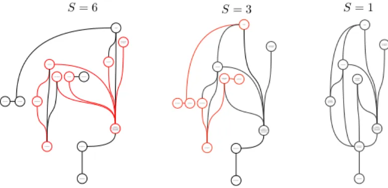
An example of a branch described at several scales is given byFigure 5. The advantage of this definition of scales for phylomemetic branches is that it endogenously adapts to the internal complexity of each branch but nevertheless makes it possible to define a scale of description for a full phylomemetic network: at scale 1, all branches have at most one cluster at each period corresponding to the synchronic merge of all the clusters of the branch at that period. For scale 𝑠 > 1, branches start branching according to their internal structure but remain in constant number.
3.2.6 Computing the ancestors beyond the time horizon
The inter-temporal matching procedure described in3.2.4may introduce artificial splits of phylomemetic branches due to the incompleteness of the corpus analyzed, such as the non-availability of digitized documents beyond a certain date. To mitigate this artifact and ease the interpretation, we have added an additional step in the reconstruction workflow that takes place in and consists in searching for common ‘ghost’ ancestors to emerging fields that have no parents. This algorithm is detailed in SIC.6and only impacts the visualization of phylomemetic networks. The reconstruction operator that takes this steps into account will be subsequently noted4Φ.
wheat
nitrogen production
dry matter cultivation crop yield
management soil organic
experiments
irrigation management practicesoil propertiescrop residue management fertilization crop rotation soil organic crop yield wheat production
dry matter cultivation
management soil organic
experiments
irrigation management practicesoil propertiescrop residue management
fertilization soil organic
crop yield crop rotationnitrogen
wheat
cultivation dry matter experiments
managementsoil organic
irrigation management practicecrop residuesoil properties managementsoil organic
fertilization crop yield
crop rotationnitrogenproduction
Figure 5: Endogenous scales of a branch. The branch wheat management of the glyphosate phylomemy ofFigure 2has
six scales of description. Here we display its internal structure at scales 1, 3 and 6. Groups and links highlighted in red are affected by changes of scale: they have either appeared, merged or divided.
4
Results
We have implemented the inter-temporal reconstruction workflow4Φas a module of the free software Gargantext15 [27] that already implements3Φ◦2Φ◦1Φ(see the details of the implementation in SIAppendix C).
We have evaluated the quality of the full workflow 𝜙 =4Φ◦3Φ◦2Φ◦1Φfrom the point of view of 𝐹
𝜆compared to results obtained by [16], as well as its capacity to provide an accurate description of the evolution of scientific domains through qualitative evaluation. The perspectives that this new methodology offers for the interaction with large set of documents through visualization are further detailed in [44].
Thereafter, we will consider for Ξ and Ψ the choices functions that seem the most consensual to us without any prior knowledge:
• Ξ(𝑥, _) is a random variable which chooses terms in with a uniform probability,
• Ψ(𝑥, _) is a random variable which chooses a branch 𝐵𝑘 ∈𝑥with a probability proportional to its number of fields.
We will see, in section6, how Ξ and Ψ can be empirically determined from specific uses and research questions.
Quality function.
Given the choices of Ξ and Ψ, the objective function 𝐹𝜆(𝜑)on 𝜑 = {𝐵𝑘}𝑘can be written withEquation 3: 𝐹𝜆(𝜑) = Σ𝑥∈ 1 ||.Σ𝐵𝑘∈𝑥𝑘 |𝐵𝑘| Σ𝐵 𝑗∈𝑥𝑘|𝐵𝑗| .𝐹𝜆(𝑥, 𝑘) (3) where: 𝑥 𝑘= {𝐵𝑘|𝐵𝑘∩𝑥≠ ∅}
4.1
Comparison with previous work
We have chosen several distinct case studies to test the robustness of our results and to illustrate the wide range of their applications. These case studies have been delineated thanks to the following corpora (see SIDfor full details).
• Domain specific academic literature.
– Glyphostate literature(seeAppendix Ffor a qualitative analysis). A corpus of 16,8k documents retrieved in the Web of Science (WoS) and PubMed. We have named this corpus 𝑔𝑙𝑦𝑝ℎ𝑜𝑠𝑎𝑡𝑒.
– Quantum computing literature. A corpus of 29k documents retrieved from the WoS. We have named this corpus 𝑞𝑢𝑎𝑛𝑡𝑢𝑚.
Table 2
Parameters for filtering cliques in each case study. Cliques of small size or with weak internal links are filtered out. The coverage column indicates the proportion of roots from that are in at least one clique in the corresponding filtered clique set .
corpus minimal clique size links threshold coverage
𝑔𝑙𝑦𝑝ℎ𝑜𝑠𝑎𝑡𝑒 7 0.001 84%
𝑞𝑢𝑎𝑛𝑡𝑢𝑚 4 0.001 80%
𝐶𝑁 𝑅𝑆 5 0.001 90%
𝐶𝑇 1 0 100 %
• Interdisciplinary academic literature. We have chosen a corpus of 6000 top-cited papers extracted from the WoS on October 2020 and for which at least one of the authors is affiliated to the National Center for Scien-tific Research (CNRS). CNRS being an interdisciplinary research organism, this corpus is by construction highly interdisciplinary and contains a limited number of documents in each discipline, yet, the phylomemy reconstruc-tion makes it possible to have an overview of the main research streams and highlights the way they combine (see [44] for a detailed description). We have named this corpus 𝐶𝑁 𝑅𝑆.
• Generic time-stamped corpora. To illustrate our method’s ability to reconstruct knowledge dynamics form any kind of time-stamped corpus as well as to process very short documents, we have applied our method to the descriptions of 6,000 arms of clinical trials related to the Covid-19. The phylomemy reconstruction highlights the different research paths and discoveries made around the Codiv-19 outbreak and could as such become a useful tool for worldwide coordination between researchers (cf. SIF.3). We have named this corpus 𝐶𝑇.
4.1.1 Workflow settings
The main parameters of the workflow 𝜙 =4Φ◦3Φ◦2Φ◦1Φhave been determined as follow:
Corpora and key-phrases extraction (
1𝜙).
For each case study, we have extracted the core vocabulary usingGar-gantext16. This core vocabulary has been further processed to compute the set of roots for each case study and their temporal co-occurrences. The corpora and the lists of terms necessary for the reproduction of this study are down-loadable from archive [59].
Similarity measures (
2Φ).
We have adopted the confidence similarity measure17which belongs to the class of syn-tagmatic similarity measures (cf. SIA). This similarity measure has proven to be a good indicator of the hypernymy / hyponymy relations between terms [28]. It is also very easy to interpret for non-specialists. Phylomemies that use such measures are reflecting actual interactions between terms and clusters in the phylomemy are generally made up of the core vocabulary of some academic sub-community.Community detection or clustering (
3Φ).
The strictest notion of cluster (or community) in a graph is the notion of clique, i.e. subsets whose elements are all linked to one another. Cliques are a fundamental and impassable level of granularity for clustering algorithms. Most clustering methods extend the notion of a cluster by relaxing the notion of a clique. Since phylomemy reconstruction generates an endogenous hierarchical clustering over a temporal series of clustering (cf. 3.2.5) we can afford to be as parsimonious as possible on the initial assumptions we make about clusters’ properties and adopt cliques as the fundamental granularity of our reconstruction.Nevertheless, all cliques are not equally relevant for the mapping of research domains, and cliques of small size (e.g. 3 or 4) or with weak internal links in most cases provide but little information and introduce some noise in the recon-struction. Moreover, keeping these weak cliques increases the number of cliques exponentially and therefore generally renders the algorithms intractable. We consequently filter the less relevant cliques according to the parameters pre-sented inTable 2andTable 3. In what follows, we will use both the maximal cliques and the frequent item sets (Fis) methods (see definitions and details in SIC.3).
16Gargantext allows an interactive selection of terms assisted by machine learning.
17The confidence between two terms 𝑖 and 𝑗 is the max of the estimation of the two probabilities of having one term given the presence of the other in the same contextual unit.
Table 3
Parameters for filtering Fis in each case study. Fis of small size or of small support are filtered out. The coverage column indicates the proportion of roots from that are in at least one Fis in the corresponding filtered .
corpus minimal Fis size minimal Fis support coverage
𝑔𝑙𝑦𝑝ℎ𝑜𝑠𝑎𝑡𝑒 7 5 11%
𝑞𝑢𝑎𝑛𝑡𝑢𝑚 4 3 52%
𝐶𝑁 𝑅𝑆 5 2 49%
𝐶𝑇 1 1 100 %
Inter-temporal matching (
4Φ).
The Jaccard similarity measure is commonly used as a means to compare sets ofelements of the same nature, making this measure a good candidate for inter-temporal matching. However, elements of clusters in phylomemies (roots) are not necessarily comparable in their usages (e.g. hyperonymes vs. hyponymes) ; which is why we have introduced a variant of the Jaccard measure to weight the contributions of roots according to their characteristics and to take into account this specificity of language. Starting with a simple adaptation, we’ve weighted the contributions of terms according to their frequency in the corpora through a sensibility parameter 𝜎 ∈ [0 1]. The chosen function Δ𝜎 is a standard Jaccard similarity for 𝜎 = 0, puts more weight on rare specific terms for 𝜎 > 0 and more weight on frequent generic terms for 𝜎 < 0:
⎧ ⎪ ⎪ ⎪ ⎪ ⎪ ⎪ ⎪ ⎨ ⎪ ⎪ ⎪ ⎪ ⎪ ⎪ ⎪ ⎩ Δ ∶∶ [−1 1] ×() × () ⟼ [0 1] Δ𝜎(𝐶, 𝐶′) = 0 𝑖𝑓 𝐶 ∩ 𝐶′= ∅ Δ𝜎(𝐶, 𝐶′) = 1 𝑖𝑓 𝐶 = 𝐶′ Δ𝜎(𝐶, 𝐶′) = |𝐶 ∩ 𝐶 ′| |𝐶 ∪ 𝐶′|𝑖𝑓 𝜎 = 0; Δ𝜎(𝐶, 𝐶′) = Σ{𝑝𝑖|𝑖∈∩(𝐶,𝐶′) 1 𝑙𝑜𝑔(𝑔(𝜎)+𝑝𝑖) Σ{𝑝 𝑖|𝑖∈∪(𝐶,𝐶′) 1 𝑙𝑜𝑔(𝑔(𝜎)+𝑝𝑖) 𝑖𝑓 𝜎 >0; Δ𝜎(𝐶, 𝐶′) = Σ{𝑝𝑖|𝑖∈∩(𝐶,𝐶 ′)𝑙𝑜𝑔(𝑔(𝜎) + 𝑝𝑖) Σ{𝑝𝑖|𝑖∈∪(𝐶,𝐶′)𝑙𝑜𝑔(𝑔(𝜎) + 𝑝𝑖) 𝑖𝑓 𝜎 <0; ; (4) where 𝑔(𝜎) = 1 𝑡𝑎𝑛(2 𝑝𝑖∗𝜎)
Phylomemies reconstructed for values of 𝜎 close to 1 will therefore tend to highlight the evolution of specific sub-domains in which clusters sharing hyponyms are likely to be related, while phylomemies reconstructed for values of 𝜎 close to -1 will tend to highlight the evolution of very generic domains where clusters sharing hyperonyms are likely to be related. The quality of these reconstructions can then be compared using 𝐹𝜆.
4.1.2 Quantitative evaluation
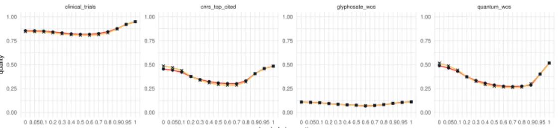
We will now compare the quality of the phylomemies obtained with the sea-level rise algorithm and the best quality that can be achieved with a uniform projector taken in {𝜋𝛿|𝛿 ∈ {0, 0.1, ..., 0.9, 1}}. We will use FIS to build series of temporal clustering ∗based on parameters taken fromTable 3.
Since by definition, uniform projectors are step phylomemetic projectors, the best step phylomemetic network is necessarily of higher quality than the best uniform phylomemetic network. However, finding the step phylomemetic network that optimizes 𝐹𝜆is done in a rugged quality landscape and is therefore a difficult task that deserves a paper in itself. The algorithm proposed in this paper can undoubtedly be improved but, as we will show, it is a good starting point.
As can be seen onFigure 6, for the various case studies and for most levels of observation 𝜆, the sea level algorithm outperforms or is at least as good as the original method. Red dots on these figures highlight the values of 𝜆 for which we the current implementation of the sea-level rise algorithm does not do better than the tested uniform projectors. For these data point at least, there are optimization margins in the way we locally increment and elect 𝛿 (see SIC.5).
We demonstrates in SIE.1that for an alternative objective function, the sea-level rise algorithm outperforms uniform step projectors all the time.
These results proves that the sea-level rise algorithm succeeds in adapting locally to the internal dynamics of the branches and in producing better precision and recall couples. Step phylomemetic networks obtained by this new algorithm should therefore be preferred over networks obtained by uniform projectors.
clinical_trials cnrs_top_cited glyphosate_wos quantum_wos
0 0.050.1 0.2 0.3 0.4 0.5 0.6 0.7 0.8 0.90.95 1 0 0.050.1 0.2 0.3 0.4 0.5 0.6 0.7 0.8 0.90.95 1 0 0.050.1 0.2 0.3 0.4 0.5 0.6 0.7 0.8 0.90.95 1 0 0.050.1 0.2 0.3 0.4 0.5 0.6 0.7 0.8 0.90.95 1 0.00 0.25 0.50 0.75 1.00 0.00 0.25 0.50 0.75 1.00 0.00 0.25 0.50 0.75 1.00 0.00 0.25 0.50 0.75 1.00 level of observation quality
projector sea level rise uniform
Quality by level of observation and projectors
clinical_trials cnrs_top_cited glyphosate_wos quantum_wos
0 0.050.1 0.2 0.3 0.4 0.5 0.6 0.7 0.8 0.90.95 1 0 0.050.1 0.2 0.3 0.4 0.5 0.6 0.7 0.8 0.90.95 1 0 0.050.1 0.2 0.3 0.4 0.5 0.6 0.7 0.8 0.90.95 1 0 0.050.1 0.2 0.3 0.4 0.5 0.6 0.7 0.8 0.90.95 1 0.8 0.9 1.0 1.1 0.8 0.9 1.0 1.1 0.8 0.9 1.0 1.1 0.8 0.9 1.0 1.1 level of observation quality r atio
Quality ratio between sea level rise and uniform projectors by level of observation
Figure 6: Comparison between the sea-level rise and uniform projectors for four distinct corpora.
4.2
External and qualitative validation
In order to assess the ability of phylomemies to fit and extend scholars expertise about knowledge dynamics of their fields, we compared in details the results of its application to two case studies: glyphosate research and research on science mapping and visualization.
4.2.1 40 years of glyphosate research
The field of glyphosate-related research (delimited by the corpus 𝑔𝑙𝑦𝑝ℎ𝑜𝑠𝑎𝑡𝑒) is particularly interesting to illustrate the relevance of our method. Literature on glyphosate is quite recent, most of it being digitized, and the knowledge it contains is of great importance from a health and economic point of view. Moreover, there is yet no consensual synthesis of the knowledge this research as produced to far. Glyphosate is a controversial herbicide about which literature reviews and historical analyses are regularly published, some emphasizing the advantages of glyphosate (e.g. [30]) or the absence of associated risks ([25,72]), others reviewing the risks for health and environment [60,45,55] and issues related to the the emergence of herbicide-resistant weeds [47].
In such scientific context, there is a high risk of selection bias when selecting publications for literature reviews and monographs, i.e. to ‘cherry-pick’ the publications that would confirm certain theoretical claims over others. In such situation, phylomemy reconstruction could be useful to give an overall picture of the field, as objective as possible inasmuch as it would include as many publications on the topic as possible and process them equally, solely on the basis of a definition of what constitutes a valid publication. Such phylomemy could highlight, before any further considerations of what is important and what is not, the main issues addressed by the scientific community and their global trends.
To compare the picture depicted by the method of phylomemy reconstruction with that depicted by experts in the field, we have synthesized the most cited literature reviews written by glyphosate supporters and skeptics [30,2,60,
34,45,55].
makes it possible to successfully identify the different research questions present in this synthesis, the details of their ramifications and their development. Full details of this analysis are provided in SI.F.
4.3
Dynamical state-of-the-art of literature related to science and knowledge mapping
The phylomemetic networks for 𝜆 = 0.3 of the knowledge dynamics corpus 𝑚𝑎𝑝𝑠analyzed in the in-depth state-of-the art of this paper (cf. SIB) is presented onFigure 7.
We can observe that this phylomemetic networks correctly describes our state-of-the-art in its temporal dimension: • The pioneer field of citation analysis was predominant during the 1970’s (branches no.1) before passing the
baton to what will become the core of bibliometry and scientometry in the early 1990’s (branches no.3). • In parallel, co-word and co-occurrence analysis [62,10] emerged in the mid 1980’s (branch 2) and enjoyed a
revival of interest in the middle of the 2000’s (branch 4) as a result of the ICT revolution. Our paper belongs to this more recent branch.
• In the mid 2000’s, the field of information retrieval developed topic modeling methods (branch 6) that were subsequently applied to digital libraries and text-classification (branch 7) as well as social media analysis (branch 8).
• At the same time, the long established field of concept mapping found concrete applications in the domains of
educationand learning process (branches 5).
2.
4.
1.
3.
5.
6.
8.
co-word analysis co-word analysis Co-citation analysis Education & learning7.
Topic modeling theory topic modelingapplications social media
analysis
Figure 7: Phylomemetic network of the literature related to science and knowledge mapping (𝑚𝑎𝑝𝑠 ) at level 0.3 with
branches smaller than 3 filtered out. Dashed boxes have been manually annotated. An interactive version of this
phy-lomemetic network available athttp://maps.gargantext.org/phylo/knowledge_visualization/memiescapeand can
be downloaded from the archive [58].
5
Discussion
5.1
Limits and continuous improvement
Phenomenological reconstruction( ⟼ ⟼ ) can lead to a misunderstanding or a biased representation of
an object 𝑂 ∈ for several reasons. First, some important observables for the understanding of 𝑂 could have been neglected or inadequately measured in the process ⟼ . Regarding the reconstruction of knowledge dynamics, this bias can be expected to diminish over time as text-mining techniques improve and as an increasing proportion of knowledge production contexts produces ever more structured and accessible digitized traces.