HAL Id: tel-01508075
https://tel.archives-ouvertes.fr/tel-01508075
Submitted on 13 Apr 2017
HAL is a multi-disciplinary open access
archive for the deposit and dissemination of
sci-entific research documents, whether they are
pub-lished or not. The documents may come from
teaching and research institutions in France or
L’archive ouverte pluridisciplinaire HAL, est
destinée au dépôt et à la diffusion de documents
scientifiques de niveau recherche, publiés ou non,
émanant des établissements d’enseignement et de
recherche français ou étrangers, des laboratoires
Regulation in commodities markets
Xiaoying Huang
To cite this version:
Xiaoying Huang. Regulation in commodities markets. Business administration. Université
Panthéon-Sorbonne - Paris I, 2016. English. �NNT : 2016PA01E004�. �tel-01508075�
UNIVERSITE PARIS 1-PANTHEON SORBONNE
ECOLE DOCTORALE DE SCIENCES DE GESTION
Labex-ReFi
Thèse: Régulation du marché des matières premières
THESE
Présentée et soutenue publiquement le 11 Avril,2016 en vue de l’obtention du Doctorat en Sciences de Gestion par
HUANG Xiaoying
Doctorant contractuel du Labex ReFi porté par heSam Université, portant la référence ANR-10-LABX-0095
JURY
Directeurs de thèse Didier Marteau
Professeur, ESCP-Europe Steve Ohana
Professeur associé, ESCP-Europe Rapporteurs Michel Albouy
Professeur, Conseiller scientifique Grenoble School of Management Yves Simon
Professeur, Université Paris-Dauphine Suffragants Gemei Aochi
Directrice des risques, Groupe Axéréal François-Gilles Le Theule
Inspecteur général de l’agriculture, Ministère de l’agriculture
Directeur exécutif, Laboratoire d’excellence sur la régulation financière Professeur affilié, ESCP-Europe
Pierre-Charles Pradier Maître de conférences & HDR,
Département d’économie (UFR 02), Université Paris 1 Panthéon-Sorbonne
Contents
Contents 2 List of Figures 4 List of Tables 5 Acknowledgement 7I General introduction
8
1 General introduction 9 Bibliography 14II Commodity prices and risk management
15
2 Behavior of French wheat prices 16
2.1 Introduction . . . 16
2.2 The features of commodity prices and related works . . . 18
2.3 The wheat market and empirical analysis of prices . . . 19
2.4 Model application and estimation results . . . 22
2.5 Diagnostic tests . . . 28
2.6 Conclusion . . . 33
Bibliography 42 3 Market risk evaluation of agricultural cooperatives 47 3.1 Introduction . . . 47
3.2 Modelling price returns and VaR . . . 49
3.3 Comparison under different scenarios . . . 54
3.4 Conclusion . . . 59
III Financialization of commodity markets
70
4 Does the impact of index flows on commodities prices involve stockpiling as a signal? 71
4.1 Introduction . . . 71
4.2 Theoretical Background . . . 72
4.3 Inventory and index funds . . . 75
4.4 Empirical Analysis . . . 79
4.5 Robustness Analysis . . . 82
4.6 Conclusion . . . 85
Bibliography 107 5 The impact of Central Banks’ announcements on commodities markets 110 5.1 Introduction . . . 110
5.2 Literature on the interaction between commodity prices and monetary policy . . . . 112
5.3 Preliminary observation . . . 114
5.4 Response of the commodity market to the Federal Reserve monetary policy . . . 117
5.5 Additional tests . . . 120
5.6 Conclusion . . . 123
Bibliography 145
IV General conclusion
147
List of Figures
2.1 Seasonality . . . 21
2.2 One example of simulated prices and original prices . . . 30
2.3 Comparison between real log return and simulated log return . . . 31
2.4 An example of prices gap between harvests . . . 34
2.5 Fundamentals of wheat market . . . 35
2.6 Daily prices series . . . 36
2.7 First-order difference of prices . . . 37
2.8 More simulation series . . . 39
3.1 Three harvests of French wheat prices from 2011 to 2014 . . . 60
3.2 Portfolio 1 - 10-Day VaR 99% . . . 61
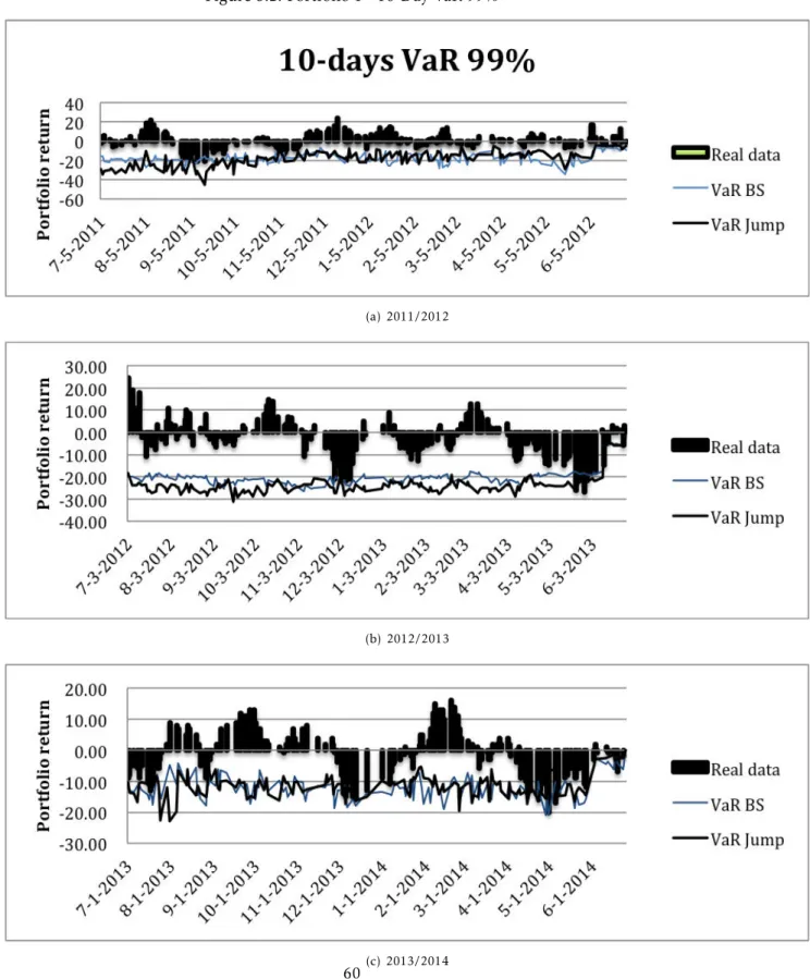
3.3 Portfolio 2 - 10-Day VaR 99% . . . 63
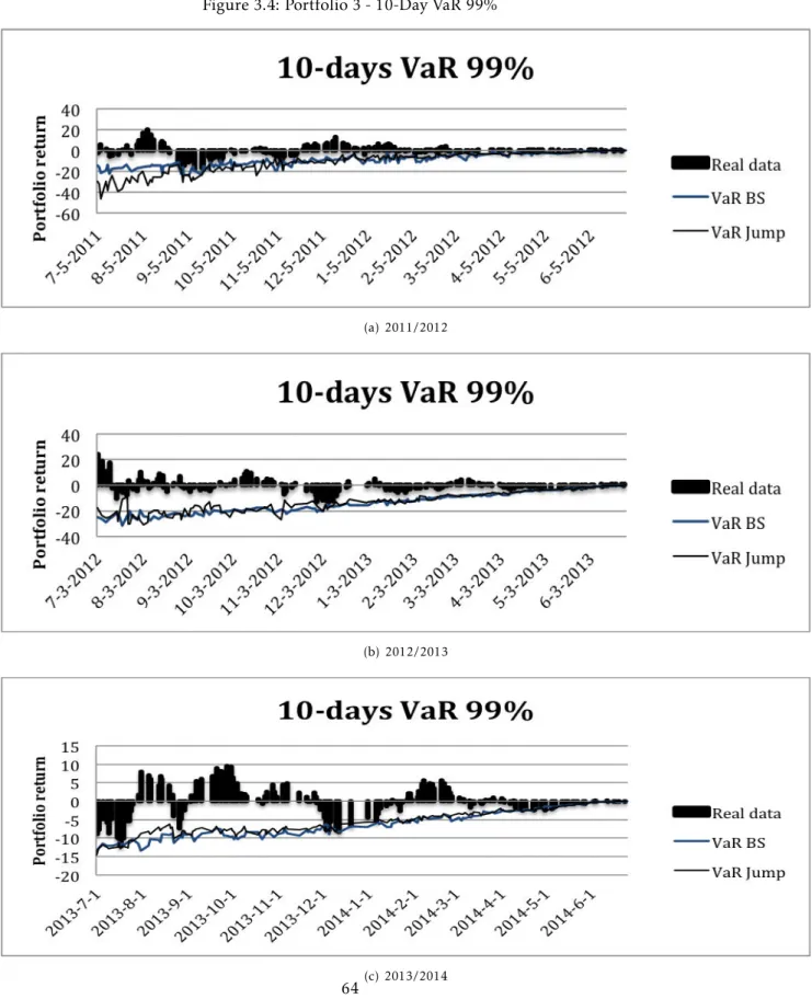
3.4 Portfolio 3 - 10-Day VaR 99% . . . 65
4.1 Relation model 1 . . . 73
4.2 Relation model 2 . . . 74
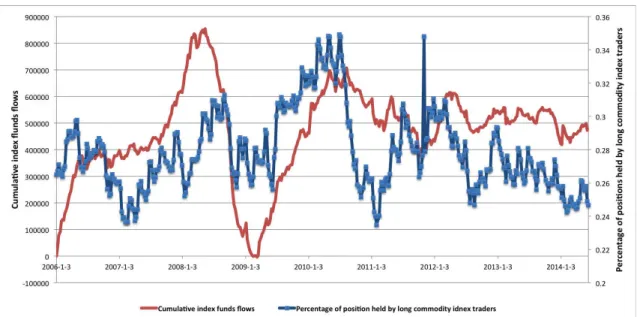
4.3 Commodity Index Funds Flows . . . 78
5.1 Commodities prices,Interest rate and Dollar index (a) and (b) . . . 125
5.2 Commodities prices,Interest rate and Dollar index (c) . . . 126
5.3 GSCI and dollar index of all trading days and of unexpected monetary policy days . . . 128
5.4 Delayed effect - Mean . . . 131
List of Tables
2.1 Descriptive statistics . . . 20
2.2 Augmented-Dickey Fuller test and Hurst exponent . . . 22
2.3 Parameter k and µx . . . 25
2.4 Parameter of volatility . . . 26
2.5 Parameters of Jump . . . 27
2.6 Likelihood ration tests(LR) . . . 28
2.7 Moments comparison . . . 32
2.8 Estimated parameters . . . 38
3.1 Portfolio 1 - Number of exceptions . . . 62
3.2 Portfolio 1 - Backtesting . . . 62
3.3 Portfolio 2 - Number of exceptions . . . 64
3.4 Portfolio 2 - Backtesting . . . 64
3.5 Portfolio 3 - Number of exceptions . . . 66
3.6 Portfolio 3 - Backtesting . . . 66
3.7 Parameters of Black-Scholes model . . . 67
3.8 Parameters of Jump model . . . 67
3.9 Basel Committee’s criterion . . . 67
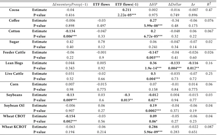
4.1 Inventory proxy and CITF . . . 87
4.2 Inventory proxy and ETF . . . 88
4.3 Inventory proxy and CITF Total . . . 89
4.4 Futures returns and CITF . . . 90
4.5 Futures returns and ETF . . . 91
4.6 Futures returns and CITF Total . . . 92
4.7 Bi-monthly regression results comparison (a) . . . 93
4.8 Bi-monthly regression results comparison (b) . . . 93
4.9 Monthly regression results comparison (a) . . . 94
4.10 Monthly regression results comparison (b) . . . 94
4.11 Specific period study: 06/2006-30/06/2008 (Commodities’ boom) a . . . 95
4.12 Specific period study: 06/2006-30/06/2008 (Commodities’ boom) b . . . 95
4.14 Specific period study: 07/2008-31/01/2009 (Commodities’ collapse) b . . . 96
4.15 Specific period study: 02/2009-31/03/2011 (Recovery) a . . . 97
4.16 Specific period study: 02/2009-31/03/2011 (Recovery) b . . . 97
4.17 Specific period study: 04/2011-2014 (Fall in commodities prices) a . . . 98
4.18 Specific period study: 04/2011-2014 (Fall in commodities prices) b . . . 98
4.19 No-agricultural commodities (a) . . . 99
4.20 No-agricultural commodities (b) . . . 99
4.21 Correlation between Stock-to-use and different inventory proxy methods . . . 100
4.22 Relationship between CITF and inventory proxy using alternative calendar spreads a) . 101 4.23 Relationship between CITF and inventory proxy using alternative calendar spreads b) . 102 4.24 Results with bi-monthly and monthly data using M1/spot spread as inventory proxy . 103 4.25 The impact of CITF using stock-to-use ratio . . . 104
4.26 Relationship between prices returns and CITF using spot prices . . . 105
4.27 Table of AIC for choosing lag number in the regression . . . 106
5.1 Correlation of major variables . . . 127
5.2 Elementary event study . . . 129
5.3 Observation before 2008: 2005/2008 (21 unexpected events) . . . 133
5.4 Observation before 2008: 2000/2005 (16 unexpected events) . . . 133
5.5 Results based on unexpected event found from inflation swap . . . 134
5.6 Transmission channels: Inventory and trading position . . . 135
5.7 Transmission channels of inventory for five individual commodities . . . 136
5.8 Role of dollar in the variation of commodity prices . . . 137
5.9 Synthesis table . . . 138
5.10 List of unexpected monetary defined from dollar index events from 2008 to 2014 . . . 139
Acknowledgement
Above all, I thank my supervisors, Pr.Didier Marteau and Pr.Steve Ohana for their support, con-fidence and patience. I would like to thank professor Marteau for spending time with me even if he has tough schecule. His advice on research has been invaluable. I would also like to thank professeur Ohana for encouraging my research and helped me come up with thesis topic. I am thankful for the excellent example both of my professors provided as a good researcher.
I thank Pr.Michel Albouy and Pr.Yves Simon for agreeing to be the reviewers and giving me feed-back to improve my thesis. I also thank Madame Gemei Aochi, Pr.François-Gilles Le Theule and Pr.Pierre-Charles Pradier, giving me the honor of being the member of jury.
I thank Labex-Refi for having financed my thesis for four years that made my Ph.D work possible. Labex-ReFi has been a source of friendships as well as good advice and collaboration, which have contributed to my personal and professional experience during my Ph.D research. I thank Pr. Le Theule, Pr.Douady and Pr. Bancel for their support in any phases of my thesis. A special thank to my friends, for sharing the best moments together during the Ph.D thesis. I am grateful for time spent with the colleges, friends in Labex and their supporting,that made my research enjoyable. I would like to thank my dad, mum and my sister for their continuous support and for staying in close contact in spite of geographical distance.
Finally, I thank Kehan for supporting and encouraging during the final stage of Ph.D. Thank you for everything.
Xiaoying Huang Paris
Part I
1
General introduction
Marchés des matières premières
Au cours de la période 2006-2008, la plupart des prix des produits agricoles se caractérisent par une forte volatilité accompagnée d’une hausse historique. Ainsi, les prix des principaux produits ont augmenté de façon spectaculaire entre 2006 et 2007, atteignant des pics extrêmes à la fin de l’année 2007 et le début 2008 pour connaître ensuite une période d’accalmie à partir de mi-2008. Puis, mi-2010, de nouveau, une phase de fortes hausses des prix est intervenue.
La hausse des prix a provoqué des problèmes sociaux, surtout auprès des pays les moins dévelop-pés consommateurs de produits alimentaires. Les prix élevés forcent les populations les plus vulnérables à réduire leur consommation, entrainant ainsi une crise alimentaire. Les décisions de production ne peuvent pas être basées sur les évolutions des prix, ce qui cause une allocation des ressources inefficaces. Par ailleurs, l’impact négatif concernant l’excès de la volatilité implique souvent l’incertitude des prix qu’elle provoque. Puis, l’excès de volatilité déstabilise le marché des matières premières, qui peut provoquer un risque systémique étant donné que les marchés des matières premières sont liés avec les autres marchés financiers tels que les marchés des ac-tions et des obligaac-tions.
Une partie de cette variation des prix est liée aux caractéristiques spécifiques des matières pre-mières agricoles. En effet, ces produits sont fortement dépendants des conditions naturelles, telles que la météo, le climat mais aussi les parasites qui peuvent décimer les cultures. En outre, l’élasticité-prix de la demande est relativement faible. Après un choc d’offre, les prix vont varier fortement afin de rétablir un nouvel équilibre. Pour ce dernier, le niveau de stockage joue un rôle important. En 2007, le stockage des produits de céréales atteint un niveau historiquement bas au plan mondial, ce qui est considéré comme l’une des raisons de la hausse des prix de ces produits sur la période.
Un ensemble de facteurs complexes issus de la modification de l’environnent économique et des marchés des matières premières, a entrainé une crise sur la période de 2006 à 2008 et sur les marchés des matières premières. L’environnement macroéconomique aux Etats-Unis s’est carac-térisé par un niveau faible de taux d’intérêt et par une politique monétaire expansionniste. La hausse des prix de l’énergie et de la dépréciation du dollar font grimper les prix des produits agricoles. Par conséquent, certains (ex : Frankel 2008) soulignent que les matières premières deviennent l’un des investissements alternatifs pour les gestionnaires de portefeuille, ce qui fait augmenter les prix. De plus, la hausse de la demande en provenance des pays émergents (la Chine, l’Inde par exemple), contribue à la hausse de prix au début 2006.
Néanmoins, ces deux facteurs expliquent difficilement l’accélération extrême de hausse de prix et de volatilité. La spéculation sur les marchés dérivés des matières premières est le plus souvent citée comme une explication de la flambée des prix à court terme. Ce facteur est lié au thème « financialization » des marchés des matières premières. La « financialization » sur ces marchés est décrite par le phénomène de co-variation entre prix des matières premières et des actifs financiers (ex : actions et obligations). L’investissement sur les matières premières permet de diversifier le portefeuille afin de réduire le risque global. Dans ce contexte, de nouveaux produits dérivés des matières premières, en particulier les fonds indiciels, contribuent à l’essor rapide et important dans le marché des commodités. Cela va causer un risque systémique et une menace pour la sta-bilité du système financier en vue de la dépendance entre les acteurs du marché et les produits de différents marchés financiers. L’analyse des facteurs individuels ne peut pas fournir une ex-plication convaincante de l’évolution des prix. Il y a encore un désaccord sur les facteurs qui se cachent derrière la crise entre 2006 et 2008 sur les marchés des matières premières.
La réponse des régulateurs
Face à la flambée des prix, à la volatilité et à l’instabilité des marchés, les régulateurs vont organ-iser des réponses portant d’une part sur la politique de stockage du marché physique et d’autre part, sur la contrainte des opérations de dérivés sur le marché financier. Plusieurs approches ont été proposées après l’épisode 2006-2008 avec un accent particulier sur les pics et volatilité des prix.
Marché physique : renforcer la transparence des informations
Dans le contexte des interventions sur le marché physique, la politique de stockage et la politique commerciale internationale sont deux outils principaux. La politique agricole commune (PAC) dans l’Union Européenne existe depuis 1960 pour la stabilisation des marchés agricoles. Son ob-jectif consiste à améliorer la productivité agricole et à protéger les bénéfices des pays membres contre des chocs externes issus du commerce international, souvent à travers des subventions. Les règlements de la PAC en 2014 se concentrent sur le bon fonctionnement des systèmes de stockage privé1.
La transparence de l’information est l’autre volet de la régulation du marché physique. A ce titre, le thème du Système d’information sur le marché des produits agricoles (AMIS) a été proposé lors du sommet du G20 2011, dans le but de recueillir des données du marché des produits agricoles et de contribuer à la transparence du marché. Dans l’attente de sa mise en place, il est également important de gérer et d’atténuer les risques pour les acteurs de ces marchés physiques qui ont le moins de connaissance en terme de finance. C’est pourquoi notre étude sur le marché physique se centre sur la gestion des risques au sein des coopératives agricoles, acteurs les plus exposés de ce point de vue.
1La contrainte est que la politique de stockage ne fonctionne pas très bien parce qu’il est difficile d’identifier les prix
appropriés. De plus, les politiques mises en place peuvent décourager la spéculation excessive, et souffrent de la même inefficience à cause de la complexité des contrats dérivés.
Marché financier des matières premières:
Superviser et contrôler l’impact des activités spéculatives
Une autre réponse face à la complexité des marchés des matières premières est l’intervention sur les marchés financiers des dérivés. Le dispositif clé des régulateurs repose sur la surveillance des activités de ces marchés afin de vérifier qu’ils assurent correctement leurs fonctions de couver-ture des risques et de formation des prix. Aux Etats-Unis, CFTC (Commodity Fucouver-tures Trading Commission) est un régulateur spécifique sur les marchés américains des futures et options qui possède une longue expérience dans la lutte contre les manipulations sur ces marchés. Dans leurs réponses et moyens d’actions, peuvent être cités en exemple : les limites de position (limiter le nombre de contrats ouverts détenus par opérateurs) ; la publication des rapports des activités des traders (CFTC publie régulièrement la situation des marchés et la répartition des positions de contrats parmi les différents acteurs du marché).
Depuis 2008, les reformes de Dodd-Frank Act et Consumer Protection Act consistent à renforcer la surveillance des marchés. Cette fois-ci, CFTC propose quelques politiques concernant les swaps qui sont des produits de gré-à-gré. La surveillance des activités des traders se fait à travers le rapport de COT (Commitments of Traders) qui inclut une nouvelle catégorie d’opérations, celles des investisseurs indiciels. Au niveau européen, la révision de la directive MiFID (Direc-tive marché d’instruments financiers), démarrée depuis 2012, contient des réglementations qui concernent les marchés financiers. Et pour la première fois, les marchés dérivés des matières premières apparaissent dans la directive. L’enjeu de MiFID est d’assurer l’intégrité et le fonction-nement des marchés des matières premières pour la couverture de prix et la formation des prix qui sont souvent la référence pour les produits physiques. De plus, les autres décisions régulatri-ces liées aux marchés des matières premières contiennent la révision de Market Abuse Directive pour la transparence des opérations ; la révision de UCITS (Undertakings for the collective in-vestment in transferable securities) pour les produits indiciels des commodités ; et la réforme d’évaluation des risques pour les banques qui tient compte des activités des matières premières. Par ailleurs, les institutions internationales ont aussi publié des rapports sur la régulation des marchés des matières premières (par ex. : IOSCO, OECD etc..). Néanmoins, les activités de ces institutions internationales se limitent aux recherches. L’application des politiques régulatrices et coopération internationale sont encore limitées.
Problématiques et structure de thèse
Les sujets portant sur la régulation des matières premières sont larges. Suite à la discussion relative à la situation et à la régulation des marchés des matières premières, cette thèse va se structurer en deux parties, le marché physique et le marché financier des matières premières agricoles et prendre trois thèmes intéressants à étudier. (i) D’une part, si les interventions sur les marchés des matières premières sont limitées, une autre option toujours ouverte est de tenter d’atténuer les impacts négatifs des comportements extrêmes des prix. Ce thème fait le point sur la gestion efficace des risques. (ii) D’autre part, à ce jour, aucun consensus n’a pu être trouvé concernant l’impact des nouveaux produits dérivés (ex : fonds indiciels). Cette question peut en fait être abordée directement dans l’impact des fonds indiciels sur le stockage des matières
premières. (iii) Enfin, parmi les régulateurs sur les marchés des matières premières, le rôle des banques centrales est souvent ignoré. Pourtant, elles peuvent aussi être un régulateur efficace sur ces marchés. S’appuyant sur ces trois points de départ, cette thèse se structure comme suit. La partie I est composée de deux chapitres qui se concentrent sur les marchés physiques et ges-tion des risques.
Chapitre 1, Etude du comportement des prix du blé, est une étude de départ qui aide à comprendre les caractéristiques des prix des produits agricoles. L’attention est portée sur les sauts extrêmes des séries des prix physiques de 2006-2014. Pour cela, un modèle stochastique de Double sauts exponentiel (Kou 2002) est appliqué. L’intérêt de ce modèle est de nous permettre de constater les comportements de sauts et de la volatilité du blé. Les résultats justifient l’évidence de sauts fréquents pour l’épisode 2007-2008 et 2010-2011. Une volatilité forte des prix est observée lors de la crise financière et lors de période comportant un choc climatique. Ce chapitre sur le com-portement des prix donne une base d’étude pour le chapitre suivant relatif à la gestion de risques et prémisse à la recherche de régulation des marchés.
Chapitre 2, Gestion des risques au sein des coopératives porte sur la prise en compte des variations extrêmes des prix sur la gestion de risques. L’indicateur de risque VaR (Value-at-Risk) est simulé avec un modèle traditionnel et un modèle de sauts. La comparaison de cet indicateur sur trois portefeuilles similaires des activités des coopératives donne la conclusion suivante : la prise en compte de sauts sur les mesures de risques peut effectivement améliorer la prévision des risques et éviter leur sous-estimation. La VaR avec prise en compte des valeurs extrêmes est un outil complémentaire dans la gestion des risques des coopératives et ne pose pas de problème de sur-coût de réservation ou de provision. Cependant, la prévision de survenance des sauts doit être prudemment étudiée.
La partie II comprend deux chapitres relatifs aux financialization du marché des matières pre-mières
Chapitre 3, L’impact des fonds indiciels, analyse l’influence potentielle de fonds indiciels sur le marché des prix agricoles. Parmi les études sur le sujet, cette étude se tourne vers la relation directe entre fonds indiciels et stockage. Nous commençons par le débat entre (Krugman, 2008) et (Pierru Babusiaux, 2010) concernant le rôle du stockage dans la relation entre spéculation et fonctionnement du marché. En vertu de régression de série temporaire, nous avons trouvé que l’impact de fonds indiciels sur le prix des matières premières est significatif à court terme mais l’impact sur le stockage n’est pas significatif. Cet impact n’a donc pas besoin de passer par le stockage à cause de l’inélasticité-prix offre et demande. Cette étude justifie la nécessité de régu-lation sur les produits indiciels des matières premières. Toutefois, le rôle des produits indiciels dans la volatilité extrême des prix physiques des matières premières reste limité. L’impact le plus important s’explique par les conditions fondamentales des marchés (climat, météo, . . . ).
Chapitre 4, La réaction des marchés des matières premières aux annonces de la banque centrale, reprend la recherche de l’impact de l’environnent macro-économique sur les marchés des matières pre-mières. L’étude met l’accent sur la réaction des indices sectoriels des matières premières sur les
communications de la Réserve Fédérale. Nous avons prouvé que les prix des matières premières deviennent plus corrélés avec les activités de banque centrale. Et cette relation repose surtout sur le taux de change et l’inflation. De l’autre coté, nous avons montré que la banque centrale peut aussi jouer un rôle dans la régulation des matières premières et ses propositions de politiques monétaires doivent aussi tenir compte des conséquences sur les marchés des matières premières. Ce sont des propositions de régulation des matières premières basées sur la compréhension des marchés des matières premières qui constitue l’objet de cette thèse.
Bibliography
[1] Frankel A.Jeffrey. (2006), The effect of monetary policy on real commodity prices. NBER Working papers series 12713.
[2] Kou S.G. (2002) A Jump-Diffusion Model for Option pricing. Management Science, Vol. 48, No. 8, pages1086-1101
[3] Krugman (2008), cite dans son bloc au Financial Times : The only way speculation can have a persistent effect on oil prices, then, is if it leads to physical hoarding – an increase in private inventories of black gunk. . . .”
[4] Pierru Babusiaux (2010), Speculation without oil stockpiling as a signature : a dyanmic perspective, OPEC Energy Review, Vol. 34, Issue 3-4, pages 131-148
Part II
2
Behavior of French wheat prices
Abstract
This paper uses a Double-exponential jump model (DEJM) including mean reversion and time-varying volatility to investigate the stochastic behavior of the daily price of wheat delivered in Rouen (France) from 2004 to 2014. The parameters are estimated separately for 10 harvests using maximum likelihood estima-tion. The main empirical results can be summarized as follows: 1) The estimated parameters among the 10 campaigns illustrate the development of wheat market and the influence from the new economic envi-ronment 2) The empirical results show that jump component and stochastic volatility do play an important role in the behavior of wheat spot prices, especially during 2007/2008 and 2010/2011. 3) by distinguishing the upward jump and downward jump, the DEJM is effective to fit the data in wheat spot prices. Likelihood ratio test and model fitting indicate also that the DEJM model outperforms alternative models. Overall, it is appropriate to consider the prices’ discontinuity in the risk measurement and management.
Keywords: Double-Exponential jump model; wheat spot price; mean reversion; stochastic volatility; likeli-hood maximization
JEL Classification:G17 Q11
2.1 Introduction
Since the 2000s, most commodities markets have been characterized by high volatility and up-ward drift. Although some commodities’ prices decreased after 2008, the price level for these commodities remains high. A few studies focus on examining the features of evolution of differ-ent kinds of commodity prices. Askari and Noureddine (2008) discuss the dynamic of oil prices that are consistent with fundamentals of the markets and global economy. Trostle et al. (2011) reexamine the recent phenomenon of food commodity and summarize the factors explaining the price surge. The relation of demand and supply is the main explanation of commodity prices, according to most studies. The objective of this paper is to analyze the variation of agricultural commodity prices during the last several years, taking here wheat as the example, and to investi-gate the price jump in french wheat market in order to discuss its risk management application. Wheat is one of the three main cereals for human food consumption. Production and prices of wheat have increased greatly with the increased demand from developing countries. The US Sen-ate Permanent Subcommittee (2009) produced a report about the excess volatility in the wheat market. The report indicates there is significant evidence that financial investment is one of the major causes of ‘unwarranted changes’. Considering the French market, production reached 36.3
million tons per year during the period 2003-2007, which is the fourth-highest rate of produc-tion in the EU. Besides the fundamental market factors, some opinions rely on the argument that this high volatility is due to the speculation in commodity derivatives markets. Recent commod-ity prices display a discontinucommod-ity evolution, which may be a reaction to an event or information, such as unpredictable weather disaster or behavior from financial market.
An understanding of the dynamics of price series is of great interest as this is a premise of mar-ket regulation, and risk management requires a further understanding of commodity spot prices modeling. The focus of this paper is to estimate a model which mimics the stochastic volatility, jumps and seasonality of agricultural commodities. With the parameters estimated, we expect to understand the reasons and the characteristics of agricultural prices. Parameters will be es-timated by using different data sets (10 harvests in total). One harvest of wheat is from July of one year to June of the next year. Wheat in different harvests would be considered as different products, since the quality could be distinct. The price gap between two different harvests can be observed from the price difference between the last opening day in June and the first opening day in July next year (Figure 2.4 of the appendix).
With the objective of identifying the jump, the application of Double-Exponential Jump model deals with the problem that commodity physical market is less liquid and probably have less fre-quent jumps than other financial markets. Comparing to other traditional jump models which usually suppose that jump size has normal distribution, this model is relevant to apply in dis-crete data. And Double-Exponential Jump model gives not only the information on jump size and frequency, but also the distinction of positive and negative jump, which is of interest in the studying of jump behaviour.
The results show that modeling the wheat spot prices using Double Exponential Jump method is flexible enough to allow to capture the special characteristics of wheat prices such as mean-reversion, time-varying volatility and jump. The French wheat prices exhibit mean mean-reversion, as most of the agricultural commodities and are volatile during several harvests. It is crucial for risk managers and policymakers to take the jump into account, since the jump term is significant according to the results.
The rest of the paper is organized as follows. In section 2, we give a summary of the characteris-tics of commodity prices and the related literature. In section 3, a stochastic model is developed to capture most of the features of agricultural commodities. In section 4, the data and some pri-mary empirical analysis of the data will be introduced. In section 5, we analyze the behavior of wheat prices by describing the estimated parameters and comment on the results. Finally, section 6 gives the conclusions and applications.
2.2 The features of commodity prices and related works
A wide range of literature has developed time series models to simulate the commodity price dy-namics. The time series models permit us to capture the accurate commodity price behavior such as skewness right, excess kurtosis and the volatility behavior. These features may be considered in the stochastic process, including mean reversion, time-varying volatility, discontinuity, etc. It is stylized empirical evidence that agricultural and other commodity prices exhibit mean re-version especially in the competitive markets framework. Under the reaction between demand and supply, commodity prices increase in the case of shortage. As a response, consumers reduce their demand so that the prices revert to supply and demand balance. The Ornstein-Uhlenbeck model first discussed by Ornstein and Uhlenbeck (1930) describes the mean-reversion feature. Bessembinder et al. (1996) point out that mean reversion is more likely to occur in agricultural commodity markets than other commodity market. Its application in commodity price modeling can be seen, for example, in Gibson and Schwartz (1990), Schwartz (1997), Schwartz and Smith (2000) and (Bernard et al.2008). They incorporate mean reversion in the drift term of the stochas-tic differential equation of spot prices.
Except at the prices level, volatility is another indicator which needs to be examined. A model without stochastic volatility could give biased estimates of the process (Crain et al. 2000). The volatility models, Autoregressive conditional heteroskedasticity (ARCH) by Engle (1982) and the Generalized Autoregressive conditional heteroskedasticity (GARCH) by Bollerslev and Ghysels (1996) are the most widely used. ARCH and GARCH models capture the excess kurtosis in com-modity price distribution, as the unconditional distribution may be not normal. Beck (2001) develops the GARCH model in the commodity market and surmises that a serially correlated price variance process exists only for storable commodities.
Concerning the distribution of price returns, empirical evidence indicates that price returns re-vealed excess kurtosis and are not normally distributed. The discontinuity of the price series (jumps/spikes)is one of the explanation of this phenomenon. Merton jump diffusion model (Mer-ton, 1976) used initially in the market is widely applied in finance, such as bonds and bond op-tions (Das & Foresi, 1996; Das, 2002) and commodity prices (Hilliard & Reis, 1998). Jumps in the price series may be the result of the unpredictable shock to the financial market or a stock-out in the commodity market. The traditional Jump-diffusion model uses the Poisson-Gaussian process: the continuous part of which is a Wiener process which measures the “normal” dynamic in prices due to relation between supply and demand; the jump component of which is a Poisson process and captures the non-continuous price dynamics. Other applications can be seen in Bernard et al. (2008, 2007)and Askari and Krichene (2008), etc. In contrast to the hypothesis of the Merton jump diffusion model, the double exponential jump model used in this paper assumes that the jump size follows a double exponential distribution, which indicates that the upward and down-ward jumps have independently exponential distribution. The model is proposed and applied in
the option pricing by Kou (2002) and Ramezani and Zeng (1998). Some empirical works in the derivatives pricing models support that the double exponential diffusion model outperforms the normal jump diffusion model (Ramezani & Zeng, 2004). Moreover, the jump size measures the price changes in response to outside news; Kou (2002) argues that the double exponential jump model captures the investors’ behavior in the overreaction and under-reaction to outside news. Based on this result, this research applies and develops the model of Kou (2002) and Ramezani and Zeng (1998) on the modeling of wheat spot prices where it also includes the feature of time-varying volatility.
2.3 The wheat market and empirical analysis of prices
The market
The data that is used is the prices of wheat delivered to Rouen. Rouen is one of the biggest ports as a delivery place for agricultural commodities for the physical market and for the financial deriva-tives market as well. A great part of French wheat production is used for exportation. France is a net-exporter country. The level of inventory in France was relatively stable from 2005 to 2012. More about production and commercial balance of wheat delivered to Rouen is given in figure 2.5 of the appendix.
By looking at the French wheat price series, it can be seen that the recent wheat market exhibits higher-level price and volatility. Figure 2.6 in the appendix gives the price series from 2004 to 2014. Prior to 2004, the wheat price is found at the lowest level, which corresponds to the re-cession in the USA. The prices swing up or down, but reverse to a mean level. The sharp price spikes during the period 2003-2004 occur due to the low amount of inventory, which is caused by unfavorable weather conditions. The prices attain a peak of 292 Euro/ton in mid-2007, and increase 100% compared to the price level in 2006. From January 2006 to April 2008, the price of wheat increase about 159%, and then decrease abruptly to the long-term level in the second semester of 2008. Meanwhile, the prices in the period of 2007/2008 become volatile compared to the previous harvest. The price changes between two business days may be 8 Euros intra-harvest, which is large in the physical market. The prices continue to fluctuate in the following two har-vests, although the average return to the level of before the financial crisis in 2008. Another peak is in 2010/2011 and compared to the summit in 2007/2008, prices are also volatile and a higher price level is maintained in the next harvest of 2011/2012, when Russia banned the exportation of wheat due to an extremely dry climate, which produces a supply shock to the global wheat market.
By also comparing between price series and the first-order difference series in figure 2.7, firstly, the first-order difference series show the existence of price jumps. First-order difference prices oscillate around zero, and some extreme price difference between two days can be observed. Sec-ondly, the effect of “Volatility clustering” is found. The higher volatility period in Figure 2.7
coincides with the higher prices of Figure 2.6, which leads to a modeling with GARCH.
Primary empirical analysis
The price series properties are first analyzed in order to establish how to model the series. The daily spot prices of wheat delivered at Rouen from 2004 to 2014 are chosen, which incorporate high volatile period of 2007/2008 and the recent peak in 2011/2012. A few arrangements are made: Firstly, the data is divided by 10 harvests, from July to June the next year, as the paper intends to study the prices harvest by harvest and considers that wheat in different harvests are distinct products, although this approach leads to decrease the accuracy of parameter estimation in the small sample. Secondly, the physical market is less liquid than the financial market. The price may not change for several days. The days in which the price is the same as the previous day are deleted.
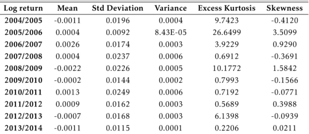
Table 2.1: Descriptive statistics
Log return Mean Std Deviation Variance Excess Kurtosis Skewness 2004/2005 -0.0011 0.0196 0.0004 9.7423 -0.4120 2005/2006 0.0004 0.0092 8.43E-05 26.6499 3.5099 2006/2007 0.0026 0.0174 0.0003 3.9229 0.9290 2007/2008 0.0004 0.0237 0.0006 0.6912 -0.3691 2008/2009 -0.0022 0.0226 0.0005 10.1772 1.5842 2009/2010 -0.0002 0.0144 0.0002 0.7993 -0.1566 2010/2011 0.0013 0.0249 0.0006 0.7192 -0.0771 2011/2012 0.0009 0.0162 0.0003 0.5689 0.3988 2012/2013 -0.0007 0.0168 0.0003 6.1398 -0.0939 2013/2014 -0.0011 0.0115 0.0001 0.2206 0.0211 Note: Descriptive statistic are calculated from log-return series for every harvests.
Descriptive statistics for the log return (defined as the difference of log prices of two opening days) is given in Table 2.1. The return series are not normally distributed, as they have non-zero skewness and positive excess kurtosis. It is justified that modeling by a simple Brownian process is ineffective.
Two years after the financial crisis of 2008, the mean returns are negative. All the returns series display a ‘fat tailed’ characteristic, with positive excess kurtosis. This evidence motivates a jump model and it is important when examining the high frequency (daily) data (Wilmot & Mason, 2011). However, another explanation of leptokurtosis is time-varying volatility. For this reason, time-varying volatility will also be considered in the following, and the likelihood ratio test will
be taken to examine the effect of time-varying volatility on the model fitting.
Figure 2.1: Seasonality
Note: The monthly averaged prices are presented below to examine the seasonality. This graph gives the monthly averaged price of the harvest: 2006/2007, 2007/2008, 2010/2011 and 2011/2012. The conclusions of other 6 harvest are the same: There is not seasonality obviously observed from the graph.
From Figure 2.1, where monthly wheat prices are presented separately, the seasonality of wheat cannot be found in the lines. According to the seasonality of agricultural products, the price is higher when it is near the harvest due to the depletion of inventories. The non-seasonality ob-served in this graph may be explained by the fact that inside one harvest the inventory of wheat can play a role of smoothing the prices. That is why in the following model estimation seasonality is not added.1
For testing the stationarity of each harvest, Table 2.2 gives the results of Augmented Dickey-Fuller tests. Hypothesis of unit-root is rejected at 5% level for all the harvest series. All log prices series are stationary, which may suggest the mean-reversion in log prices. The mean-reversion property is also verified with the calculation of Hurst exponent.
1It should be noted that the seasonality is taken into account by a trigonometric function in the beginning of this
work; however it is difficult to find the parameters with the optimization algorithm and, even if the estimated parameters were found, the results were inconsistent and impossible to interpret.
The Hurst exponents obtained by R/S analysis with log prices series of every campaign are smaller than 0.5 and significant at the 5% level according to the t-stat. On the basis of Hurst exponent, the wheat prices have a mean-reversion behavior.
Table 2.2: Augmented-Dickey Fuller test and Hurst exponent ADF-test Test critical value: 5% level
07/2004-06/2005 -6.7787 -1.9421 07/2005-06/2006 -5.6823 -1.9421 07/2006-06/2007 -17.1640 -1.9421 07/2007-06/2008 -8.2637 -1.9421 07/2008-06/2009 -17.0044 -1.9420 07/2009-06/2010 -4.4711 -1.9423 07/2010-06/2011 -9.3745 -1.9477 07/2011-06/2012 -6.2747 -1.9736 07/2012-06/2013 -4.1501 -1.9424 07/2013-06/2014 -1.3184 -1.9425
Hurst exponent t-stat 07/2004-06/2005 0.4358 8.58E-21 07/2005-06/2006 0.2077 3.44E-07 07/2006-06/2007 0.3107 7.06E-30 07/2007-06/2008 0.3350 3.23E-23 07/2008-06/2009 0.4293 1.28E-33 07/2009-06/2010 0.2319 1.43E-22 07/2010-06/2011 0.2890 2.88E-33 07/2011-06/2012 0.4053 2.41E-32 07/2012-06/2013 0.3927 1.69E-15 07/2013-06/2014 0.2681 1.14E-12
Note: These two tests are taken on the log prices series. Lag numbers of ADF-test are chosen by AIC/BIC criteria.
2.4 Model application and estimation results
Model application
In this model, the log price is assumed to follow a Brownian motion with a mean-reversion term, plus a compound Poisson process with jump sizes double exponentially distributed (Kou, 2002; Ramezani & Zeng, 1998). This model allows to study the positive and negative jumps respec-tively. Volatility is supposed to be stochastic (GARCH). With Xt= ln(St), log prices and Vt= σt2,
volatility:
dXt= κ (µx− Xt)dt+ σtdBt+ JtdNt (2.1)
dVt= κv(µv− Vt)dt+ σvVtdBvt (2.2)
Xt= ln(St), log prices can be stated by a Jump-diffusion process which is presented by an
Ornstein-Uhlenbeck process plus a Poisson term.
In equation (2.1) and (2.2), the Ornstein-Uhlenbeck process captures the mean-reversion behav-ior of prices. k denotes the rate that the log prices Xtreturn to a equilibrium or a mean value µx; Volatility�Vt= σt2
�
is supposed to be stochastic. The volatility with GARCH behavior is modeled as a mean-reversion process. The Brownian motion Btand Bvt, following Nt∼ (0, dt) are assumed to be independent.
Jump
The discontinuous component of the price process is described by a Poisson counter Nt in the equation (2.1), with intensity λ and jump size Jt. The intensity λ is the average number of jumps
per unit of time, which can also be explained as the probability that jump occurs, Prob (∆Nt= 1) = λdt and probability of no jump, Prob (∆Nt= 0) = 1 − λdt.
When the jump occurs, the log price jumps from X(t−)to Xt= Jt+ X(t−). We know that Xt= ln(St), so ln (St) = Jt+ ln � S(t−) � , or St= e(Jt)S(t−). We have �
eJt�− 1, the percentage change of the prices. The double exponential distribution of Jtis supposed to be independent of Btand Bvt. It is the Jt
that illustrates the leptokurtic of the price returns. The double exponential distribution of Jtis:
fJt= η1e−η1Jt Probability = p (2.3) η2eη2Jt Probability = 1 − p (2.4) The probability p, is the probability that an upward jump occurs, and 1-p is the probability of a downward jump. According to the exponential distribution, the means of exponential random variables are 1/η1and −1/η2for positive and negative jump sizes respectively. The mean of Jt is
obtained easily, which is equal to p/η1− (1 − p)/η2. The jump size is not normally distributed but
has the leptokurtic feature. And the Double Exponent Jump model (DEJM for simplicity in the rest of this paper) gives the feature of overreaction and under-reaction to outside news and also the reaction to good or bad news; “DEJM can be interpreted as an attempt to . . . incorporate in-vestors’ sentiment” (Kou 2002). And the hypothesis of double exponent jump is more practically applied in illiquid market with discrete jumps. In this case, the two types of jump are supposed to be independent for simplification.2
Volatility
From equation (2.2), the specification of volatility is a continuous case of GARCH (Brockwell and Chadraa 2006). For facilitating estimation, we can re-write Vt = ω + αε2t−1+ βVt−1with εt−1the
error term at time t-1; ω > 0 et α ≥ 0,β ≥ 0; and α + β < 1 (stationary condition). Transforming to the continuous form of GARCH, we have kv= 1 − α − β and σv= α
√
2 (Daniel B. 1990).
The equation of volatility, Vt, is the discrete form of GARCH, where1 − α − βω measures the
long-run average variance per day by using the daily data here. Using the square-root-time rule, the annualized volatility may be calculated by
� ω 1 − α − β
√
252; α + β is the persistence of volatility. Likelihood function
For the likelihood function, the density of Xtis simplified as a Bernoulli weighted sum of normal and exponential density. The three sources of randomness, Bt,Bvt and Nt, are assumed to be
in-dependent. Price processes are divided into two regimes: Jumps happen with probability λ; No jumps with probability 1 − λ.
Define a random variable Xtas a sum of independent normal (with mean µ and variance σ2) and
exponential (with parameter δ) random variables. Its density function is:
g�X��=δ 2e δ 2 � 2µ+δσ2 −2X�� erf c � −µ + δσ2− X� √ 2σ � , (2.5)
where erf c (x) the complementary error function =√2 π
�∞
x e−s
2 ds Then density function can be written also as:
g�X��= δe δ 2 � 2µ+δσ2−2X�� Φ X �+µ−δσ2 σ
, with Φ (): Cumulative distribution CDF of standard normal variables.
The density function of Xtcombined with a Bernoulli distribution in our case can be calculated
(see also Ramezani and Zeng (1998) and Kou (2002)):
f(Xt) = λ � pη1e σ2η12 2 e−(X(t)−(1−κ)X(t−1)−κµx)η1Φ � − (X (t) − (1 − κ) X (t − 1) + κµx− Vtη1) √ Vt � +(1 − p)η2e σ2η22 2 e−(X(t)−(1−κ)X(t−1)−κµx)η2Φ � (X (t) − (1 − κ)X (t − 1) + κµx− Vtη2) √ Vt �� +(1 − λ)√1 2πe − (X (t) − (1 − k)X (t − 1) − κµx)2 2Vt (2.6)
The log likelihood function to be maximized is: L (P) =�T
t=1ln [f (Xt)] with T the last trading day
of the sample.
Parameters P = (κ,µx, p, η1, η2, λ, ω, α, β) can be estimated by maximization of the likelihood
func-tion numerically3. Positive value constraints are put on all the parameters. The initial parameters
are chosen carefully since results are highly dependent on the initial values.
Estimation results
Table 2.8 in the appendix gives the results from the maximum likelihood function. Parameters are given by different harvest periods (10 harvests in our sample). All the estimated parameters are significant, with the level at least 10%. The standard errors reported are calculated using the Hessian matrix. The tables below, which provide explanation of different behavior, are extracted from Table 2.8 of the appendix.
Mean-reversion behavior
Table 2.3: Parameter k and µx
k 1/k µx eµx
Speed of returning to mean Days of returning to mean Equilibrium log price Equilibrium price 2004/2005 0.0218 45.9144 4.5803 97.5435 2005/2006 0.0908 11.0189 4.6426 103.8187 2006/2007 0.0514 19.4561 4.9601 142.6130 2007/2008 0.0191 52.4271 5.4882 241.8283 2008/2009 0.0169 59.3109 4.7776 118.8126 2009/2010 0.0600 16.6652 4.7706 117.9878 2010/2011 0.0363 27.5373 5.5063 246.2511 2011/2012 0.0903 11.0761 5.2870 197.7559 2012/2013 0.0200 49.997 5.2874 197.829 2013/2014 0.0725 27.5781 5.4492 232.5602
κ presents how quickly the log-price reverts to its long-run mean in the log-price process and 1/κ is the days to return to the equilibrium level (The transformation of number of days is based on the opening days). Prices in the harvest during 2007/2008 and 2008/2009 revert to mean more slowly than in other years, where it takes more than 50 days (two months). Another period, 2004/2005, also takes about 45 days to revert to the long-run level, which may be explained by the lower storage pressure in the previous harvest and the market uncertainty. In both 2004/2005 and 2008/2009, the prices do not return to the equilibrium level as quickly as other periods, one of the potential explanations is that during these harvests inventory is relatively lower.
Regarding the equilibrium level of prices, the mean price is coherent with price variation and re-flect the commodity inventory adjustment. Peaks are in 2007/2008, 2010/2011 and 2013/2014, where prices tend to be about 241.8 Euros/ton. The 2007/2008 harvest coincides with the crisis from the financial industry. As a result, the explanations of the 2007 peak consist of the increasing demand from emerging countries and the financialization of the commodity markets according to several researches. Then, the price peak in 2010/2011 is probably due to Russia’s exportation ban, which put pressure on the international wheat market. The difference between 2007/2008 and 2010/2011 harvests is that we observe that, after 2010/2011, the equilibrium price remains relatively high after the peak of the previous year; however, prices drop down dramatically in the harvest following 2007/2008.
Volatility behavior
Table 2.4: Parameter of volatility
ω α β α + β � ω 1 − α − β √ 252 Persistence of volatility Mean volatility 2004/2005 0.000079 0.2625 0.0078 0.2703 0.1651 2005/2006 0.000011 0.6161 0.0427 0.6855 0.0915 2006/2007 0.000087 0.0921 0.4389 0.5309 0.2163 2007/2008 0.000155 0.2045 0.4439 0.6484 0.3331 2008/2009 0.000103 0.0205 0.6489 0.6695 0.2797 2009/2010 0.000088 0.0282 0.4277 0.4559 0.2017 2010/2011 0.000024 0.1917 0.7643 0.9560 0.3720 2011/2012 0.000003 0.0040 0.9740 0.9780 0.1891 2012/2013 0.000150 0.1464 0.0415 0.1879 0.2157 2013/2014 0.000095 0.10 0.1119 0.2119 0.1740
The volatility is a little bit smaller than the volatility calculated4in the descriptive statistic table
and in the traditional lognormal model, since part of volatility is interpreted by the jump term in our model. The volatility obtained by the GARCH model measures the ‘normal’ price variation, which is caused by fundamental conditions. In spite of this, the evolution path of volatility is the same, with highest yearly mean volatility of 33% in 2007/2008 and 37% in 2010/2011. The high volatility implies uncertainty in the wheat market and the market is sensitive to exogenous information. It is surmised that the uncertainty in 2007/08 comes from the tremors in the finan-cial market and relatively small harvest. And the supply shock in the international market due to Russia’s exportation ban may be a main cause of high volatility during 2010/2011.
Another highly volatile campaign is the 2004/2005 harvest, which may be a result of the histor-ically lowest inventory in 2003/2004. The tension of the supply side due to unfavorable climate in the previous year caused the uncertainty to remain in the 2004/2005 harvest. Conforming to the simple statistical analysis, the volatility in 2008/2009 remains higher although the price decreases from the peak. Moreover, after another summit in 2010/2011, the prices vary less vi-olently. Using the specification of GARCH, volatilities in all harvests are not persistent (α + β < 1). Jump behavior
Table 2.5: Parameters of Jump
p 1 η1 − 1 η2 1 λ Probability of upward jump Mean of upward jump Mean of downward jump Number of jumps 2004/2005 0.5577 0.0716 -0.0835 7.1011 2005/2006 0.5354 0.0284 -0.0162 7.6126 2006/2007 0.7965 0.0376 -0.0347 15.8074 2007/2008 0.3013 0.0595 -0.0589 14.4927 2008/2009 0.4989 0.0667 -0.0478 14.2818 2009/2010 0.5013 0.0300 -0.0325 16.6618 2010/2011 0.4600 0.0589 -0.0578 16.5967 2011/2012 0.5798 0.0358 -0.0327 12.3731 2012/2013 0.400 0.0667 -0.0667 16.66 2013/2014 0.5872 0.0250 -0.0333 24.99
The jump is distinguished by upward and downward jump. The table above gives the results of jump parameters. The mean of jump is defined as the averaged difference between ln (St) and
ln�S(t−1)�, if jump occurs. Jumps have happened more frequently since 2006. 2005/2006 has the smoothest trait with no-frequent and small jumps. Prices increase from 2006 and oscillate along a high level during 2007/2008. The probability of an upward jump is larger than a downward jump, with p = 0.79 in 2006/2007. The upward jumps are dominant in this period. Although prices remain higher in 2007/2008, the downward jumps occur more often.
Otherwise, two kinds of cases can be distinguished according to the results: Firstly, the harvest of 2004/2005 is categorized by jump with large size and lower frequency. Secondly, in the years 2006/2008 and 2010/2011, the jumps happen more frequently but have lower value. The results of the jumps are confirmed with those of mean reversion and volatility: In the higher volatile period, the jumps are more frequent and prices deviate to the market equilibrium much longer than in other periods. In 2004/2005, the jumps may be caused by the fundamental conditions, which provoke a large change in the wheat price. According to the previous results, the first two harvests in our sample are dominated by the fundamental information (inventory status), while the smaller and lower frequency jumps in 2007/2008 and 2010/2011 may be explained by supply shock from domestic and international market. The surmise of impact from the financial market should refer to more rigorous analysis.
2.5 Diagnostic tests
In this section, robust tests will be taken to examine the validation of the model. The objective is to investigate if the mean reversion, jump behavior and time-varying volatility are appropriate to fit wheat spot prices. For answering this question, likelihood ratio tests are taken with three alternatives models under different hypotheses; and four moments calculated from the simulated prices series are compared with the moments by original data.
Likelihood ratio tests
Table 2.6: Likelihood ration tests(LR)
Without jump Without mean reversion Constant volatility MC p-value
2004/2005 49.579 9.620 6.896 0.01 2005/2006 59.963 1.907 3.109 0.01 2006/2007 29.470 5.923 5.890 0.01 2007/2008 13.224 4.042 23.254 0.01 2008/2009 39.970 1.227 1.844 0.01 2009/2010 8.486 2.511 32.174 0.01 2010/2011 4.991 8.152 23.492 0.01 2011/2012 2.865 1.033 1.596 0.01 2012/2013 18.571 1.492 2.058 0.01 2013/2014 4.343 3.770 1.148 0.01
Note: Likelihood ratios are calculated for every harvest by comparing with the models without jump, models without mean reversion and models with constant volatility
The likelihood ratios are calculated by estimating three other models, which are ARCH model with stochastic volatility (without mean reversion); Mean-reversion model with stochastic volatil-ity (without jump term); and Jump diffusion model with constant volatilvolatil-ity (without stochastic volatility). We are interested only on the LR-test. The results of parameters are not given in this paper.
Simply comparing the likelihood values does not permit us to choose the fitted model, as the model with the larger number of parameters may have a higher likelihood value. The three groups of likelihood ratios are calculated in the table.
Likelihood ratio is defined as LR = −2[L(�p, X) − L (P,X)], with�p the parameters estimated by re-stricted models, P the parameters estimated by the complete model, and X the log prices. LR is Chi-square distributed with k degree of freedom (k is the number of restrictions).
We can see that the hypothesis is rejected. Compared to all alternative models, the initial model (DJEM) is significant. It is effective to investigate the wheat prices by the complete model
accord-ing to the likelihood ratio test. Moment fitting
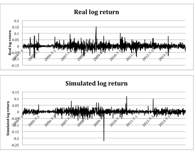
The prices will be simulated using the estimated parameters. Then the moments are calculated by the new simulated series. The comparison will be taken between the original moments and the moment simulated. Firstly, the simulated series and the original series are taken in the same graph, as shown in figure 2.2.
Figure 2.2: One example of simulated prices and original prices
Note:The original prices are presented by the solid curve and one of the simulated prices is shown by the point curve.
Figure 2.3: Comparison between real log return and simulated log return
Note: The log returns in the simulated log-return graphs are calculated from the simulated prices.In the simulation we have simulated 1000 series, which constitute a surface around the real prices line. Only the simulated series below 10% standard deviation and above 10% standard deviation are considered.
Figure 2.3 shows only one simulated series, which is considered the closest to the real data series. The estimation and simulation are produced by a discontinuity Poisson process and for every har-vest. The simulated prices and log returns fit the real data during 2005/2006, which is also the most stable period among the 10 harvests. The deviation between the simulated series and the original is much higher in the high volatility period. It should be noted that the real data depends also on the economic conditions and outside information, and the simulated price series depends only on the assumptions of time series. As in the simulation process, a Poisson distribution sim-ulates the jump with a well-defined frequency. However, concerning the jump size, whether it is an upward or downward jump, the estimation is conducted by the mean of the jumps size. As a
result by simulation, the jumps happen randomly without considering the real information from the market.
Table 2.7: Moments comparison
Mean Variance Kurtosis Skewness Simulated Original Simulated Original Simulated Original Simulated Original 2004/2005 -0.0005 -0.0011 0.0037 0.0004 1.8414 9.7423 -0.1168 -0.4120 2005/2006 0.0004 0.0004 0.0004 8.43E-05 1.0896 26.6499 1.3459 3.5099 2006/2007 0.0026 0.0026 0.0090 0.0003 4.2099 3.9229 -0.7021 0.9289 2007/2008 0.0009 0.0004 0.0192 0.0006 2.0985 0.6912 -0.3561 -0.3692 2008/2009 -0.0022 -0.0022 0.0215 0.0005 10.9567 10.1772 0.8724 1.5841 2009/2010 -0.0004 -0.0002 0.0026 0.0002 7.0331 0.7993 0.2725 -0.1567 2010/2011 0.0030 0.0013 0.0156 0.0006 50.7101 0.7192 -1.3379 -0.077 2011/2012 -0.0005 0.0009 0.0033 0.0003 3.7895 0.5689 -0.366 0.3988 2012/2013 -0.0019 -0.0007 0.0002 0.0003 0.2688 6.1398 2.8415 -0.0943 2013/2014 -0.0006 -0.0011 0.0001 0.0001 0.1555 0.2206 3.1607 0.0216 Note: Four moments are calculated:mean, variance, kurtosis and skewness from original log-return series and simulated log-return series.
The four moments for 10 harvests are obtained in Table 2.7. The first two moments do not di-verge too much from the original data. In contrast, simulated skewness and kurtosis are much smaller than the original. The explanation of this fact can also be due to the lack of assumption about the economic condition in the simulation. Another 3 simulation series are given (Figure 2.8) in the appendix. The deviation between real data and simulated data always exists for the high volatility period. And these simulated series are quite different from each other given the random simulation. At least, the simulated series replicate the main features of real data, such as mean reversion, and higher volatility for certain harvests.
A brief conclusion of this section: The model used in this article is to capture the key features of wheat prices. Using mean reversion, jump process and varying volatility is effective according to the simple likelihood ratio tests. Chan (2005) finds similar results about short-term interest rate: that models combining mean reversion, jump and time-varying volatility fit the data, and the conclusion of Ramezani and Zeng (2004) for stock market is mixed. The simulation cannot produce a similar series during the high volatility period as a result of complicated market con-ditions. The first two moments are coherent with the original moments. It should be mentioned that the skewness and kurtosis are unstable according to different series. After taking all the above into account the complete model (DEJM) used in this paper is effective to investigate the trait of wheat spot prices and to be applied in the market with less and discrete jumps observed.
2.6 Conclusion
In this paper, a stochastic jump process is used to capture the French wheat spot prices from 2004 to 2014. The stochastic process incorporates almost all the categories of price variation, including mean reversion, jump behavior and varying volatility. The modelling of jump as an exponential distribution deals with the problem of less liquidity in physical market and allow to distinguish between positive and negative jump. The parameters are estimated by a numerical maximization of the likelihood function. Estimation is taken by different harvests independently. In the end, there are 10 groups of parameters to interpret. Several robust tests are taken after estimation. It is reasonable to incorporate the mean reversion and jump term into the process. The focal point is to study the wheat spot prices features that can be found from the analysis.
At first, the wheat prices exhibit the mean-reversion behavior: after a shock on the prices, the prices will return to an equilibrium level. However, the time taken to return depends on the mar-ket condition. During the volatile period (2007/2008 and 2010/2011), prices fluctuate far from equilibrium level. Secondly, the period of 2007/2009 exhibits higher volatility for French wheat. The changes in inventory and influence from other countries do have an impact on the French wheat market, since the market is never only domestically confined. As a result, fundamental condition is still the main explanation of the fluctuation of wheat prices. Thirdly, 2007/2008 dis-plays more frequent downward and small jumps. In addition, compared with the early years, the wheat market undergoes more shocks from the outside, with more jumps happening. Finally, the fundamentals seem still to be able to provide the major explanation of the volatility, as supply shock provoke higher volatility in respective periods. However, harvests with frequently jump happening coincide with the periods of financial crisis. This fact leads to the conjecture of impact from financial markets.
The finding in this paper gives us some features of wheat prices and is relevant for the regula-tors. According to the results of our modeling, it is crucial that the agricultural cooperatives and the policymakers take the jump into account in their risk management strategies. However, the results of this paper are not enough to justify the impact of “financialization” or precise factors on the wheat market. Which are the factors behind the volatile prices? Are the fundamental con-ditions (supply/demand) dominant in the agricultural market or does the speculation from the commodity derivatives market produce the recent price changes? All the questions not concluded in this paper will be discussed in future research.
Appendix Figure 2.4: An exam ple of prices gap betw een harv ests Note: The gr aph giv es the prices betw een harv ests 2004/2005 and 2005/2006. The last opening da y for 2004/2005 is 27th June and the fi rst opening da y for 2005/2006 is 1st Jul y. The black curv e linked these tw o poin ts in the gr aph. There are apparen t price chang es on these tw o da ys. A similar phenomenon ma y also be found in other years. In this paper ,the estima tion is carried out on 10 harv ests separ atel y by considering whea t from di fferen t harv ests as distinct prod ucts (di fferen t qualities).
Figure 2.5: Fundamen tals of whea t mar ket Note: The exporta tion, im porta tion and total output of the French soft whea t mar ket from 2004 to 2014 are giv en in this gr aph (y -axis: 1000 tons/unity). As a prod ucer coun try ,F rench im porta tion is small. A bout half of output is used for export. The lev els of prod uction and exporta tion of 2007/2008 are rela tiv el y small com pared to other years.(Sources:A greste)
Figure 2.6: Dail y prices series Note: The gr aph giv es the dail y spot prices (E uro/ton) of French soft whea t and it is also the da ta tha t are used in the paper . The sam ple period is from 2004 to 2014, 10 harv ests in total. Bef ore 2006, prices varied smoothl y al ong 100 E uros/ton and increased after tha t un til reaching a peak in 2007. The prices oscilla ted betw een 300 E uro/ton and 200 E uro/ton d uring 2007 and 2008. Then whea t prices decreased after 2008 but main tained vola tility .The recen t high prices beg an in 2010 and are char acterized also by a high vola tility .
Figure 2.7: First -order di fference of prices Note: The gr aph giv es the fi rst order di fference of prices. The higher vola tility period is seen to coincide with the higher prices period which begins on Jul y 2006. The fact justi fi es the existence of “V ola tility cl ustering” which is represen ted by a G ARCH model.
Table 2.8: Estima ted par ameters C am pagne k µx p η1 η2 λ ω α β -Log Likelihood 2004/2005 V al ue 0.0218 4.5796 0.4011 28.1493 24.5404 0.0489 8.10E-05 0.2867 0.0059 -452.7 std error (3.66E-03) (1.05E-02) (0.0021) (0.0901) (0.0126) (0.0023) (1.25E-05) (5.13E-03) 2.14E-03 2005/2006 V al ue 0.1003 4.6478 0.5398 63.8271 87.1363 0.0507 8.49E-06 0.1985 0.5775 -453.95 std error (8.91E-03) 4.24E-03 0.0266 0.9895 1.00 0.0303 1.62E-02 3.38E-02 5.45E-02 2006/2007 V al ue 0.0403 4.9832 0.5997 28.1841 36.2241 0.0310 2.84E-05 0.1379 0.6682 -607.8 std error (6.15E-03) (3.23E-02) (0.0515) (1.03) (1.03) (1.2E-02) (7.24E-06) (3.03E-02) (0.0463) 2007/2008 V al ue 0.0239 5.4754 0.451 23.603 21.1662 0.035 0.0002 0.2119 0.3798 -527.1 std error (0.0052) (0.0771) (0.8920) (1.2288) (1.69) (0.0210) (2.53E-05) 0.0564 0.0508 2008/2009 V al ue 0.0226 4.8342 0.4339 17.9475 23.6587 0.0634 1.04E-04 0.0212 0.6463 -498.2 std error (9.92E-03) (0.0579) (0.0412) (1.09) (1.42) (0.0406) (1.16E-05) (0.0183) (0.0351) 2009/2010 V al ue 0.0600 4.7706 0.5013 33.3163 30.7647 0.0600 8.79E-05 0.0282 0.4277 -570.05 std error (0.0015) (1.21E-02) (0.3746) (1.0048) (1.01) (2.21E-02) (4.20E-06) (0.0129) (5.88E-02) 2010/2011 V al ue 0.0606 5.4719 0.6165 26.8196 19.2339 0.0472 3.51E-05 0.2012 0.7367 -514.4 std error (0.0106) (2.09E-02) (0.1105) (0.9451) (1.01) (0.0364) 1.15E-05 (0.0433) (0.0307) 2011/2012 V al ue 0.0903 5.2874 0.5798 27.9485 30.9311 0.0601 3.19E-06 0.0040 0.9743 -419.7 std error (2.26E-02) (1.29E-02) (0.3540) (4.7725) (0.0331) (0.0573) (7.01E-07) (2.90E-03) (3.08E-03) 2012/2013 V al ue 0.0200 5.4491 0.400 15.00 14.996 0.0600 1.50E-04 0.1464 0.0415 -492.2 std error (6.66E-03) 4.15E-02 (0.0145) (0.4089) (0.0365) (0.0226) (2.14E-05) (1.78E-02) (1.26E-02) 2013/2014 V al ue 0.0725 5.2110 0.5872 39.997 29.9998 0.0300 9.47E-05 0.1000 0.1119 -489.4 std error (1.34E-02) (5.28E-02) (0.185) (10.4418) (9.74) (0.0464) (1.17E-05) (8.95E-02) (8.9E-02) Note: This table giv es all estima ted par ameters using maxim um likelihood function. Standard error giv en in paren theses is cal cula ted by Hessian ma trix. All the par ameters are signi fi can t – at least 10% lev el. In the estima tion, sign constr ain ts are giv en on all par ameters for in some cases neg ativ e val ue is fr aud.
Figure 2.8: More sim ula tion series Note: This gr aph giv es 3 sim ula ted series. s1, s2, s3 represen t the 3 sim ula ted series of log prices and the black thick curv e is the real da ta series. In the 2010/2011 harv est , it seems tha t the sim ula ted series cannot arriv e to the same high lev el as the real one. The prices are low er at the beginning of the harv est com pared to the end of the harv est. The property of mean rev ersion prod uces a sim ula ted curv e varying al ong an equilibrium lev el, which is low er than the higher prices of the middle harv est. Y -axis is the log prices.
Annex: Estimation using Matlab
In the following, we give the estimation code using maximum likelihood function in Matlab en-vironment for the first year data of 2004/2005.
load(’Camp.mat’) 1) Optimization function St=Camprest(:, 1);
t = Camprest(:, 2);
options = optimset(�Algorithm�,�Interior − point�,�MaxIter�, 500);
- Initial parameters should be chosen firstly:
parametre=[0.02 4.6 0.45 30 28 0.03 0.0001 0.01 0.01]’;
- Constraint conditions on certain parameters and t-value for significance test is applied with Hessian matrix obtained from the function:
[parametre,likeli,exitf lage,output,lamdba,grad,hessian] = f mincon(@(parametre)like1(parametre,St,t),parametre, [000000 − 100;0000000 − 10;00000000 − 1],[0;0;−0.001],[],[],[],[],[],options); stanerr=sqrt((diag(hessian)).∧ − 1); tstat = parametre./stanerr; p1=parametre(1);p2=parametre(2); p5=parametre(6);p10=parametre(3);p11=parametre(4);p12=parametre(5); p6=parametre(7);p7=parametre(8);p8=parametre(9);
2) Define the vt: volatility would be a vector with length of St vt(1)=0.0004; vt(2)=0.0005; for i=3:157; vt(i)=p6+p7*(St(i-1)-St(i-2)-p1*(p2-St(i-2)))2+ p8 ∗ vt(i − 1); end mj=p10/p11-(1-p10)/p12; vj=p10*(1-p10)*(1/p11+1/p12)2+ p10/(p112) + (1 − p10)/(p122);
3) Define the likelihood function fun = @(x) exp(-x.2/2);
for i=2:157;
X(i)= -(St(i)-St(i-1)-p1*(p2-St(i-1))-vt(i)*p11)/(vt(i)0.5)
Y (i) = (St(i) − St(i − 1) − p1 ∗ (p2 − St(i − 1)) − vt(i) ∗ p12)/(vt(i)0.5) q(i) = integral(f un, X(i), Inf )
p(i) == integral(f un, Y (i), Inf )
Lt(i)=log((1-p5)*exp(-(St(i)-St(i-1)-p1*(p2-St(i-1)))2/(2 ∗ vt(i)))/(2 ∗ pi ∗ vt(i))0.5 + p5 ∗ (p10 ∗ p11 ∗
exp(vt(i) ∗p112/2) ∗exp(−(St(i)−St(i −1)−p1∗(p2−St(i −1)))∗p11)∗q(i)+(1−p10)∗p12∗exp(vt(i)∗ p122/2) ∗ exp((St(i) − St(i − 1) − p1 ∗ (p2 − St(i − 1))) ∗ p12) ∗ p(i));
Bibliography
[1] Alexander Carol and Emese Laxar,2005, On The Continuous limit of GARCH. Working paper. [2] Angus Deaton and Laroque Guy,1996, Commodity storage and commodity price dynamics.
Journal of Political Economy, Vol. 104, No.5, 896-923.
[3] Angus Deaton and Laroque Guy,1992, On the behavior of commodity prices. The Review of Economic Studies, Vol. 59, Issue 1, 1-23.
[4] Barry K. Goodwin, Schnepf Randy and Dohlman Erik,2005, Modelling soybean prices in a changing policy environment. Applied Economics, Vol. 37, Issue 3, 253-263.
[5] Feldman Barry and Till Hilary,2006, Backwardation and commodity futures performance: Evidence from evolving agricultural markets. The Journal of Alternative Investments, Vol.9, No.3, 24-39.
[6] Stacie Beck,2001, Autoregressive conditional heteroscedasticity in commodity spot prices. Journal of Applied Econometrics, Volume 16, Issue 2,115-132.
[7] Jean-Thomas Bernard; Lynda Khalaf; Maral Kichian; and Sebastien McMahon. 2008, Oil prices: Heavy tails, Mean Reversion and the Convenience yield. Working paper, Bank of Canada & Quebec Ministry of Finance, 2008.
[8] Jean-Thomas Bernard; Lynda Khalaf; Maral Kichian; and Sebastien McMahon.2008, Fore-casting Commodity Prices: GARCH, Jumps, and Mean Reversion. Journal of ForeFore-casting, 27, 2008: 279-291.
[9] Hendrik Bessembinder;Jay F. Coughenour; Paul J.Seguin and Margaret Smoller.1996, Is there a term structure of futures volatilities? Reevaluting the Samuelson hypothesis. The Journal of Derivatives, Vol.4, No. 2, 45-58.
[10] Michael J. Brennan 1958, The supply of storage. The American of Economic Review Vol. 48, No.1, 50-72, 1958.
[11] Peter Brockwell ; Chadraa Erdenebaatar and Alexander Lindner. 2006, Continuous-time GARCH processes. The Annals of Applied Probability Vol. 16, No.2,790-826.
[12] Sorensen Carsten.2002, Modeling seasonality in agricultural commodity futures. The Journal of futures markets Vol.22, Issue 5,393-426.