HAL Id: hal-00563461
https://hal.archives-ouvertes.fr/hal-00563461
Submitted on 18 Jul 2012
HAL is a multi-disciplinary open access
archive for the deposit and dissemination of
sci-entific research documents, whether they are
pub-lished or not. The documents may come from
L’archive ouverte pluridisciplinaire HAL, est
destinée au dépôt et à la diffusion de documents
scientifiques de niveau recherche, publiés ou non,
émanant des établissements d’enseignement et de
Communities of Minima in Local Optima Networks of
Combinatorial Spaces
Fabio Daolio, Marco Tomassini, Sébastien Verel, Gabriela Ochoa
To cite this version:
Fabio Daolio, Marco Tomassini, Sébastien Verel, Gabriela Ochoa. Communities of Minima in Local
Optima Networks of Combinatorial Spaces. Physica A: Statistical Mechanics and its Applications,
Elsevier, 2011, 390 (9), pp.1684 - 1694. �10.1016/j.physa.2011.01.005�. �hal-00563461�
Communities of Minima in Local Optima Networks of
Combinatorial Spaces
Fabio Daolioa, Marco Tomassinia, S´ebastien V´erelb, Gabriela Ochoac
aFaculty of Business and Economics, Department of Information Systems, University of Lausanne,
Switzerland
bINRIA Lille - Nord Europe and University of Nice Sophia-Antipolis / CNRS, Nice, France
cAutomated Scheduling, Optimisation and Planning (ASAP) Group, School of Computer Science,
University of Nottingham, Nottingham, UK
Abstract
In this work we present a new methodology to study the structure of the configuration spaces of hard combinatorial problems. It consists in building the network that has as nodes the locally optimal configurations and as edges the weighted oriented tran-sitions between their basins of attraction. We apply the approach to the detection of communities in the optima networks produced by two different classes of instances of a hard combinatorial optimization problem: the quadratic assignment problem (QAP). We provide evidence indicating that the two problem instance classes give rise to very different configuration spaces. For the so-called real-like class, the networks possess a clear modular structure, while the optima networks belonging to the class of random uniform instances are less well partitionable into clusters. This is convincingly sup-ported by using several statistical tests. Finally, we shortly discuss the consequences of the findings for heuristically searching the corresponding problem spaces.
Key words: Community structure; Optima networks; Combinatorial fitness landscapes
PACS:; 89.75.-k; 89.75.Fb; 75.10.Nr
1. Introduction
In the last decade some researchers have proposed a network view of energy land-scapes in chemical physics for small atomic clusters and macromolecules [1, 2, 3]. The idea is simple: if one can identify both the minima of these energy landscapes and
the possible transitions between them, then one can build a graph in which the nodes are the minima and the transitions are represented by edges joining the corresponding minima [2]. The number of minima usually increases exponentially with system size but significant samples can be obtained either by experiment or, much more often, by sampling the landscape using molecular dynamics and Monte Carlo methods (see [4] and references therein). Doye has called this graph the Inherent Structure Network; here we prefer to use the term Local Optima Network (LON).
Inspired by this approach, in our own work [5, 6] we have applied similar ideas to the case of the configuration spaces of difficult combinatorial optimization problems. Although the problems look superficially similar, hard combinatorial spaces pose addi-tional challenges due to their discrete nature, e.g. no derivatives and gradient informa-tion is available. Moreover, the landscapes are rugged, may show frustrainforma-tion, i.e. not all local constraints can be satisfied together in order to improve the objective function value, and often contain neutrality which means that there are sizable regions where the objective function values are identical or very close to each other. The typical physical models that show most of these features are spin glasses [7] but the phenomenon is ubiquitous in combinatorial spaces of computationally hard problems [8].
Assuming that the LON of the given combinatorial landscape is known, or at least a significant sample has been obtained, several questions are of great interest, both the-oretical and practical. First and foremost, the distribution over the search space of the optima and their connectivity, as well as the associated basins of attraction and their sizes, are fundamental information that may help to understand the difficulty of the cor-responding problem and may guide local search methods through the problem config-uration space. Second, the number and strength of possible transitions between basins, and thus between optima, are also extremely important to gauge the stability of local optima configurations and the possibility of jumping out of a suboptimal configuration to reach a better one, or even the globally optimal one. Several other purely topologi-cal features of such a landscape representation are also very useful. For example, the mean path length between any local optimum to the global one contains information about the computational difficulty of the problem. The clustering coefficient of the op-tima network is also interesting as it gives information about the topological transitivity
between related optima.
In the present study we focus on a particular fundamental characteristic of the op-tima networks using the Quadratic Assignement Problem (QAP), which is a typical member of the class of computationally hard problems [8]. The feature we are inter-ested in, is related to the way in which local optima are distributed in the configuration space. Then, several questions can be raised. Are they uniformly distributed as some theoretical analyses of fitness landscapes seem to assume for mathematical simplic-ity [9], or do they cluster in some non-homogeneous way? If the latter, what is the relation between objective function values within and among different clusters and how easy is it to go from one cluster to another? Knowing even approximate answers to some of these questions would be very useful to further characterize the difficulty of a class of problems and also, potentially, to devise new search heuristics or variation to known heuristics that take advantage of this information.
There exist some measures that are used to characterize numerically distributions of landscape features such as average solution distance and average distance between optima, where the distance is seldom the usual Euclidean one but rather another kind of distance such as Hamming distance for problems defined on binary string configura-tions, or the distance between two permutations in a permutation space [10]. However, a purely topological vision may offer several advantages with respect to such “met-ric” approaches since in the former only information about the vertices of the graph and their connections is needed. In complex network theory language, the above cor-responds to the detection of communities in the relevant LON networks. Community detection is a difficult task, but today several good approximate algorithms are avail-able and the approach is feasible, especially for the small networks studied here [11]. A similar investigation has been performed by Massen and Doye [12] for the graphs of energy landscapes of small atomic clusters and by Gfeller at al. for continuous free-energy landscapes in biomolecular studies [13].
The present study is structured as follows. In order to make the article sufficiently self-contained, we first briefly describe the QAP problem and introduce our concepts and methods to define and find the LONs. We next describe in detail the community search approach and we discuss the results obtained on two different classes of QAP
problem instances and their significance. Finally, we give our conclusions.
2. The QAP Problem
The QAP deals with the relative location of units that interact with one another in some manner. The objective is to minimize the total cost of interactions. The problem can be stated in this way: there are n units or facilities to be assigned to n predefined locations, where each location can accommodate any one unit. Location i and location j are separated by a distance aij, generically representing the per unit cost of interac-tion between the two locainterac-tions. A flow of value bij has to go from unit i to unit j; the objective is to find and assignment, i.e. a bijection from the set of facilities onto the set of locations, which minimizes the sum of products flow × distance.
This bijection can naturally be encoded as a permutation π and the problem of cost assignment minimization can mathematically be formulated as:
min π∈P (n) C(π) = n X i=1 n X j=1 aijbπiπj (1)
where C(π) is the cost function, A = {aij} and B = {bij} are the two n × n distance and flow matrixes, πigives the location of facility i in permutation π ∈ Σn, and Σnis the set of all permutations of {1, 2, ..., n}, i.e. the QAP search space. The structures of the distance and flow matrices characterize the class of instances of the QAP problem. Later in the article it is explained which are the classes of instances used in the present work.
3. Local Optima Networks
Given a fitness landscape for an instance of a combinatorial optimization problem like the QAP, we have to define the associated optima network by providing definitions for the nodes and the edges of the network. The vertexes of the graph can be straight-forwardly defined as the local minima of the landscape. In this work, we select small QAP instances such that it is feasible to obtain the nodes of the graph exhaustively by running a best-improvement local search algorithm from every configuration of the
search space as described below. Before explaining how the edges of the network are obtained, a number of relevant definitions are summarized.
A Fitness landscape [14] is a triplet (S, V, f ) where S is a set of potential solutions, i.e. a search space, V : S −→ 2S, a neighborhood structure, is a function that assigns to every s ∈ S a set of neighbors V (s), and f : S −→ R is a fitness function, also called cost function or objective function, that can be pictured as the height of the corresponding solutions. In our study, a search space configuration s is a permutation π of the n facility locations, therefore the search space size is n!. The neighborhood of a configuration is defined by the pairwise exchange operation, which is the most basic operation used by many meta-heuristics for QAP. This operator simply exchanges any two positions in a permutation π, thus transforming it into another permutation. The neighborhood size is thus |V (s)| = n(n − 1)/2. Finally, the fitness for this problem is defined by equation 1 as f (s) = −C(s).
The Best Improvement (BI) algorithm to determine the local optima and therefore define the basins of attraction starts from an arbitrary configuration s and systematically tries to improve the solution by looking at all neighbor solutions V (s), choosing the best one. It stops when no improvement is possible, i.e. when the current solution s∗ is a local optimum: ∀s ∈ V (s∗), f (s) < f (s∗).
The basin of attraction of a local optimum i ∈ S is the set bi= {s ∈ S | BI(s) = i}. The size of the basin of attraction of a local optimum i is the cardinality of bi. The basins of attraction as defined above produce a partition of the configuration space S. Therefore, S = b1∪ b2∪ . . . ∪ bnand ∀i 6= j, bi∩ bj = ∅.
We can now define the weight of an edge that connects two feasible solutions in the fitness landscape. For each pair of solutions s and s0, p(s → s0) is the probability to go from s to s0 with the given neighborhood structure. For the search space of permutations of n elements, and the pairwise exchange operation, there are n(n − 1)/2 neighbors for each solution, therefore:
if s0∈ V (s) , p(s → s0) =n(n−1)/21 and if s06∈ V (s) , p(s → s0) = 0.
is defined as:
p(s → bj) = X
s0∈bj
p(s → s0).
Notice that p(s → bj) ≤ 1. Thus, the total probability of going from basin bito basin bjis the average over all s ∈ biof the transition probabilities to solutions s
0 ∈ bj: p(bi→ bj) = 1 |bi| X s∈bi p(s → bj), where |bi| is the size of the basin bi.
Now we can define a Local Optima Network (LON) as being the graph G = (S∗, E) where the set of vertices S∗contains all the local optima, and there is an edge eij∈ E with weight wij = p(bi→ bj) between two nodes i and j iff p(bi → bj) > 0. Notice that since each maximum has its associated basin, G also describes the interconnection of basins.
According to our definition of edge weights, wij = p(bi → bj) may be different than wji = p(bj → bi). Thus, two weights are needed in general, and we have an oriented transition graph.
4. Structure of the QAP LONs 4.1. Problem Instance Generation
In order to perform a statistical analysis, several problem instances of at least two different problem classes have to be considered. To this purpose, the two instance generators proposed by Knowles and Corne [15] for the multi-objective QAP have been adapted and used here for the single-objective QAP. The first generator produces uniformly random instances where all flows and distances are integers sampled from uniform distributions. This leads to the kind of problem known in literature as Tainna, being nn the problem dimension [16]. Distance matrix entries are, in both cases, the Euclidean distances between points in the plane. The second generator permits to ob-tain flow entries that are non-uniform random values. This procedure, detailed in [15]
produces random instances of type Tainnb which have the so called “real-like” struc-ture since they resemble to the strucstruc-ture of QAP problems found in practical appli-cations. For a general network analysis, 30 random uniform and 30 random real-like instances have been generated for each problem dimension in {5, ..., 10}. To the spe-cific purpose of community detection, 200 additional instances have been produced and analyzed with size 9 for the random uniform class, and size 11 for the real-like in-stances class. Problem size 11 is the largest one for which an exhaustive sample of the configuration space is computationally feasible. Beyond that, sampling must be used. However, in this work we prefer to stick with exact results in order to give as accurate as possible answers to the minima clustering problem posed at the beginning.
4.2. Network Analysis
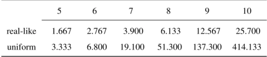
The results of the statistical analysis of the above QAP landscapes, up to size 10, appear in [17] to which the reader is referred for further information. In that work it is shown that LONs for the QAP are dense, as one can see from Tables 1 and 2 which give, respectively, the mean number of vertices and the mean number of edges for the two classes of instances and for instance sizes going from 5 to 10.
Table 1: Average values of the number of vertices for each instance size.
5 6 7 8 9 10
real-like 1.667 2.767 3.900 6.133 12.567 25.700
uniform 3.333 6.800 19.100 51.300 137.300 414.133
Table 2: Average value of the number of edges for each instance size.
5 6 7 8 9 10
real-like 3.400 9.433 19.900 46.0667 187.433 818.700
Table 3 shows that the LONs of both the uniform and real-like instances up to size 10 are complete or almost complete since |E| = O(|V |2). This is inconvenient for community analysis as it is difficult for any cluster detection algorithm to split-up the networks into separate communities when the graphs are so dense.
Table 3: Average of the ratio of the number of edges to squared number of vertices
5 6 7 8 9 10 real-like 1.000 0.993 0.994 0.999 0.992 0.988 uniform 0.998 0.993 0.969 0.940 0.9087 0.874 5 6 7 8 9 10 0.0 0.2 0.4 0.6 0.8 1.0 Problem Dimension A ve ra ge T ra ns it ion P roba bi li ty Wii Wij 5 6 7 8 9 10 0.0 0.2 0.4 0.6 0.8 1.0 Problem Dimension A ve ra ge T ra ns it ion P roba bi li ty Wii Wij
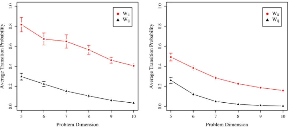
Figure 1: Average weights wiifor self-loops (circular points) and wijfor out-going links (triangular points).
Left image: real-like instances. Right image: uniform instances. Bars depict 95% confidence intervals on the means (standard errors). Averages from 30 independent and randomly generated instances are shown.
However, looking at Fig. 1 which gives the average values of the transition prob-abilities to stay in the same basin and to jump to another basin, it is apparent that most of the probability distribution is placed in p(i → i), i.e. it is more likely for a solution to stay in the same basin rather than to jump to a neighboring one for both instance classes. When a local stochastic heuristic is used to search the landscape, only transitions to another basin that have higher probability of occurring are important.
Ac-tually, a search heuristic like simulated annealing also accepts moves that worsen the objective function with low probability, but the acceptance rate decays quickly as the temperature is lowered and, in the end, only the most likely transitions play a role. In fact, the important role that “weak ties” may have in a social network context [18] is almost absent in combinatorial landscapes where the more probable search paths are associated with the highest transition probabilities when these landscapes are searched with a local stochastic heuristic. These considerations give us a clue as to how to filter out the network edges in such a way that only the more likely transitions are kept and, as a consequence, the graph becomes much less dense and gives a coarser but clearer view of the fitness landscape backbone. Such a network can be used for community analysis. On the other hand, it is also possible to keep the original dense weighted directed networks and to use a specialized community detection algorithm that was originally designed to work in such cases, which is called the Markov Clustering Algo-rithm(MCL) [19]. We first explain our filtering procedure in the following and then we will compare the results with those obtained through the MCL algorithm. Nevertheless, we point out that, even in the MCL case, the algorithm itself does some preprocessing of the network weights.
The filtering procedure is very simple. First, we transform the weighted directed graph G into a weighted undirected one Guby taking each pair of edges ~ij and ~ji and replacing them with a single undirected link ij whose weight is the average:
wij = ~
wij+ ~wji
2 .
Indeed, the values of ~wijand ~wjiare different in general and thus taking a single edge is an approximation. However, a local heuristic walking the landscape would still be able to traverse a link in both directions, whereas filtering the directed edges could cause some transitions to disappear.
Now, on Guwe establish a probability threshold Π for the weights wij associated to each edge in Gu = (S∗, E) and suppress all edges that have wij smaller than the value marking the Π-quantile in the weights distribution. We call the resulting network G0u = (S∗, E0); it has the same number of vertices as Gu and a number of edges
|E0| ≤ |E|.
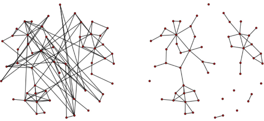
The following Figures 2 and 3 show an example of the results of such a filter-ing process, startfilter-ing from the LON of a particular instance and for four values of the threshold Π.
Figure 2: Left image, edge pruning threshold Π = 0.50, right image Π = 0.75.
Figure 3: Left image, Threshold Π = 0.91, right image Π = 0.95; in this case the graph becomes discon-nected.
How to choose the threshold Π is essentially a matter of trial and error. Too low a value does not allow a crisp picture of the network to emerge; but if Π is too high the network finally falls apart into separated components as in Fig. 3 which is not acceptable since, by definition of fitness landscape, the whole graph must be connected.
Likewise, if some node becomes isolated during filtering, it cannot be simply removed since it could, at least in principle, be the configuration corresponding to the global optimum. Thus, each analyzed network has been filtered up to the maximum value of Π that still preserves its connectivity.
4.3. Communities of Optima in LONs
Communities or clusters in networks can be loosely defined as being groups of nodes that are strongly connected between them and poorly connected with the rest of the graph. Several methods have been proposed to uncover the clusters present in a network (for an excellent recent review see [11]). Community detection belongs to the class of graph partitioning problems, which are hard in the sense that there is no known algorithm bounded by a polynomial function of the size of the input to exactly solve the problem [8]. Community detection has the added difficulty that there is not a single accepted rigorous measure of a cluster or a partition of the nodes of a given graph into meaningful clusters. One commonly used measure is Modularity. The modularity Q of a partition has been defined as a merit function measuring the fraction of within community edges minus the expected value of such fraction for a randomized network with the same vertex degree distribution [20].
Several heuristics have been proposed [11]; after a preliminary analysis, we have chosen two of them: Clauset et al’s. method based on greedy modularity optimiza-tion [21], and Reichardt’s and Bornholdt’s spin glass ground state-based algorithm [22]1. Both methods gave consistent results on our networks and, in addition, they also work with undirected weighted networks which was required in our case. The reason for using two methods is that we can assess statistical significance independent of the al-gorithm and we can double check the community partition results.
For the sake of the community analysis we shall use only the results on newly generated problems of size 11 for the real-like instances and of size 9 for the uniform random ones. This is suggested by the consideration that the LONs for these two cases
1For the actual computations and data treatment, the “igraph” complex network analysis package [23],
rl.1 uni.1 rl.2 uni.2 0.1 0.2 0.3 0.4 0.5 0.6 0.7 0.8 M odul ari ty Q
Figure 4: Boxplots of the modularity score Q on the y-axis with respect to class problem (rl stands for real-like and uni stands for random uniform) and community detection algorithm (1 stands for fast greedy modularity optimization and 2 stands for spin glass search algorithm).
have comparable sizes in terms of number of vertices and can still be obtained exactly by an exhaustive search. The resulting networks are still relatively small: the average size is 60 for real-like instances and 127 for random uniform ones but already sufficient for a meaningful cluster analysis. For example, they have sizes larger than the famous “Zachary’s Karate Club Network” [25], which has 34 nodes and is routinely mentioned as a standard benchmark in community detection work [11].
Before examining the actual community structures found, we present the results of some tests in order to evaluate the statistical significance of the clustering in terms of modularity.
In general, the higher the value of Q of a partition, the crisper the community struc-ture. Figure 4 is a plot of the modularity score Q distribution empirically determined from the data for each algorithm/problem class pair. The boxes “hinges” represent the 25, 50 (thick lines), and 75% quantiles. The plot indicates that the two problem
classes are well separated in terms of Q, and that the community detection algorithm does not seem to have any influence on such a result. To further show that these results are statistically significant, we have performed a permutation test [26] for a factorial ANOVA design, modeling the modularity scores as a response variable to the prob-lem class and algorithm choice. The p-values thus obtained are 2 × 10⁻⁴, 0.179, and 0.6414 for the factor “problem class”, factor “algorithm”, and the interaction between the two, respectively. Only the first one is below the significativity threshold of 0.05. It is thus safe to conclude that the data show no significant effect of the community de-tection method used on the variability observed in modularity score, while the problem class only seems to explain that variability: real-like instances can be clustered in more modular partitionings than random uniform ones.
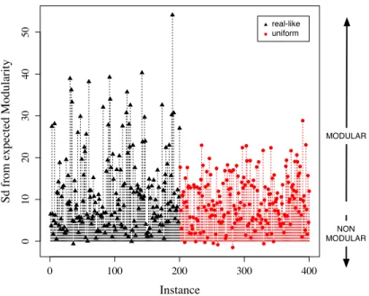
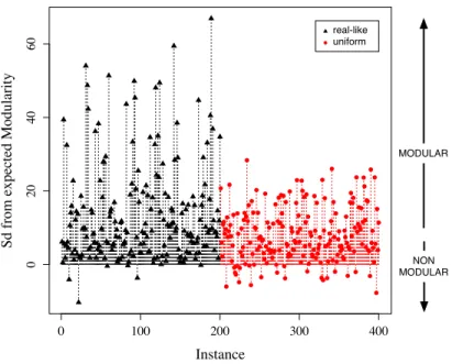
0 100 200 300 400 0 10 20 30 40 50 Instance S d from e xpe ct ed M odul ari ty MODULAR NON MODULAR real-like uniform
Figure 5: Modularity Q for the best clustering into communities by means of greedy optimization algorithm. For each instance (x-axis: 200 real-like ones on the left, 200 random uniform ones on the right), Q is plotted in number of standard deviations (y-axis) away from the average of 1000 randomised networks with the same degree sequence.
0 100 200 300 400 0 20 40 60 Instance S d from e xpe ct ed M odul ari ty MODULAR NON MODULAR real-like uniform
Figure 6: Modularity Q for the best clustering into communities by means of spin glass model algorithm. For each instance (x-axis: 200 real-like ones on the left, 200 random uniform ones on the right), Q is plotted in number of standard deviations (y-axis) away from the average of 1000 randomised networks with the same degree sequence.
However, modularity scores alone can be misleading. This has been shown by Guimer`a et al. in [27] where they pointed out that many random networks with no clear community structure may nevertheless have rather high values of Q due to sta-tistical fluctuations. Thus, to test for the stasta-tistical significance of Q we used a Monte Carlo procedure in which a randomized version of the data is produced. For each prob-lem instance, 1000 random networks have been generated using Viger’s and Latapy’s algorithm [28], i.e. starting with the original graph’s degree sequence and rewiring the links randomly without altering the sequence. Next, both community detection algo-rithms have been applied to each generated network to obtain the modularities Q of their partitions. Finally, a p-value has been computed by comparing the expected value of Q from the randomized networks with the Q measured for the actual original
net-work. Among the 200 considered real-like instances, those p-values are not significant in 14 and 22 cases when using the two community finding algorithms. Among the 200 random uniform instances, the non-significant cases are 16 and 36, respectively. These figures are slightly higher than “5-out-of-100” ratio one could expect from the signifi-cance threshold, but not by a margin high enough to invalidate the results of the whole analysis. In conclusion, a separation between the two problem classes, with respect to minima clustering in the search space, has been significatively highlighted.
Once the significance of a community structure has been assessed, in order to have an insight into its strength, one can also measure for each instance how distant the obtained modularity score is from the expected value estimated on the respective null model. Networks observed in nature and society present a modularity structure not only significantly different but markedly higher than random networks [29]. In this respect, Figures 5 and 6 depict for each instance the difference in number of standard deviations (with respect to the 0 horizontal line) between the measured modularity scores and the expected ones for the null model (a population of 1000 randomized networks having the same degree sequence, as explained above). It is worth stressing that the absolute value of such a distance depends on the variability observed within the null models. Nonetheless, there is difference between the two problem classes, with real-like ones displaying a stronger and more instance-dependent community structure than random uniform ones, disregarding the algorithm chosen to discover such a structure.
To end this section, we now briefly present the results obtained through the use of the MCL algorithm, as explained in sect. 4.2. In Fig. 7 we report the modularity scores for the two algorithms we used on the weighted undirected filtered networks (greedy modularity optimization and spin-glass model), and for MCL on the complete weighted and directed LONs.
To be able to compare modularity scores in a consistent way, we took each algo-rithm’s best found community subdivision and we computed the weighted variant of its Q value on the original unfiltered networks. From the figure, we observe that the results are qualitatively the same, i.e. real-like instances give rise to optima networks with a more modular structure than uniform ones, even if MCL’s results have higher
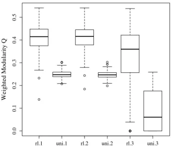
rl.1 uni.1 rl.2 uni.2 rl.3 uni.3 0.0 0.1 0.2 0.3 0.4 0.5 W ei ght ed M odul ari ty Q
Figure 7: Weighted modularity scores Q for the best community clusterings found by the greedy optimization algorithm (left), by the spin-glass ground-state algorithm (center), and by the MCL algorithm (right). The first two are applied to the filtered and undirected but weighted graphs, whereas MCL applies to the original unfiltered weighted and directed ones.
variance and for uniform instances sometimes no community is found at all. Indeed, MCL faces very dense networks and, to get useful results, the algorithm rescales link weight values in a preprocessing phase. In the end, we feel that both methods give comparable results but filtering out the networks and then searching for clusters gives rise to more stable partitions.
4.4. Discussion
From all the previous statistical tests it is apparent that real-like instances have significantly more cluster structure than the class of random uniform instances of the QAP problem. This can be appreciated visually by looking at Figs. 8 and 9 where the community structures of the LON of two particular instances are depicted. Although these are the two particular cases with the highest Q values of their respective classes, the trends observed are general.
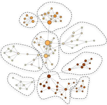
Figure 8: Community structure of the LON of a real-like instance. The cluster partition found is highlighted. Node sizes are proportional to the corresponding basin size. Darker colors mean better fitness (lower).
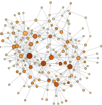
Fig. 8 shows the minima community structure of an instance of the real-like class. One can see that groups of minima are rather recognizable and form well separated clusters (encircled with dotted lines), which is also reflected in the high corresponding modularity value Q = 0.79. Contrastingly, Fig. 9 represents a case drawn from the class of random uniform instances. The network has communities, with a Q = 0.53, although they are hard to represent graphically, and thus are not shown in the picture.
In the figures, the diameter of the nodes is drawn proportional to the size of the corresponding basin of attraction in the fitness landscape. As for the fitness values, the lower (better) the value, the darker the node is. In [17] it was found that there is a positive correlation between fitness values and the corresponding basin size, especially for the random uniform problem instances. This effect is qualitatively easy to spot on the figures. The results of this community study, together with [17], sheds light on an open problem in the structure of difficult combinatorial landscapes. The basin
Figure 9: Cluster structure of the LON of a random uniform instance. Clusters are less well separated (see text) and cannot be clearly highlighted. Node sizes are proportional to the corresponding basin size. Darker colors mean better fitness.
sizes of these problems have been often taken either constant or uniformly distributed at random for mathematical reasons of simplicity [9]. However, this is far from being the case for the QAP problem [17] and the NK landscapes [30, 5] at least. While this conclusion cannot be generalized easily, it could also hold for other families of difficult combinatorial problems based, as the QAP, on permutation neighborhood such as the Traveling Salesman Problem (TSP) for example.
From the point of view of the clustering of solutions in the problem fitness land-scapes, it has been conjectured that QAP landscapes fall essentially into two classes: non-structured, with local optima randomly scattered through the search space, and “massif central”, with the optima clustered into few localized regions [31]. The sug-gestion was based on sampling the fitness landscapes with random walks and measur-ing entropy and mean distances among local optima. Our community analysis supports
and goes beyond this intuition providing a richer and fitness-independent global view of the full mesoscopic structure of the solutions network.
To complement the previous purely topological view, it is useful to investigate the correlation of fitness values between neighboring vertices in the unfiltered LONs. Fig-ure 10 shows scatterplots of the correlation between the fitness of a given node and the average fitness of its first neighbors in the graph. The plots correspond to the two particular cases shown in Figs. 8 and Fig. 9. It is apparent that the network is definitely assortative with respect to fitness in the real-like case and slightly so in the uniform case. Indeed, regression lines show that the correlation is positive in both cases but it is higher in the real-like one, which also has a lower variance. Although we show results for two particular networks here, we have computed averages over all networks and the trend is the same: in the unfiltered case we get a Spearman correlation coeffi-cient r = 0.7677 for the real-like instance class and r = 0.3992 for the uniform one. The regression-line slopes are, respectively, 0.249 and only 0.055. Interestingly, for the filtered backbone networks, fitness becomes disassortative for uniform instances (r = −0.3459) whereas it is still assortative for the real-like case (r = 0.2286) .
-3000000 -2500000 -2000000
-2600000
-2400000
-2200000
-2000000
Fitness of the local optimum
W ei ght ed a ve ra ge of ne ighbors ' fi tne ss -215000 -210000 -205000 -200000 -206000 -205000 -204000
Fitness of the local optimum
W ei ght ed a ve ra ge of ne ighbors ' fi tne ss
Figure 10: Scatterplots and regression lines of the mean fitness of the nearest neighbors of a vertex having fit-ness f . Left image: real-like instance corresponding to Fig. 8. Right image: uniform instance corresponding to Fig. 9. Mean neighbor fitness is weighted with the transition probabilities of the corresponding outgoing links.
Although it is outside the scope of the present study, we should like to mention that the above results may have deep consequences on the heuristics used to search combinatorial spaces such as those described here. For example, in the case of random uniform instances, the landscape has little structure with a small range of fitness values, so that a standard local search heuristic such as best improvement or first improvement will quickly find a satisfactory solution. In contrast, in the landscapes generated by real-like instances, there will be almost separated groups of minima and thus a parallel-search heuristic that simultaneously explores several regions of the parallel-search space, or a restart strategy like iterated local search, could be more effective. Also, in this case the use of a non-local move operator would perhaps be beneficial.
5. Summary and Conclusions
In this work, we have presented a new methodology to study the structure of the configuration spaces of hard combinatorial problems. It essentially consists in build-ing the network which has as nodes the locally optimal configurations and as edges the weighted oriented transitions between optima. In particular, here we applied the approach to the detection of communities in the optima networks produced by two different classes of instances of the QAP, which is a hard combinatorial optimization problem. We provided evidence for the fact that the two problem instance classes give rise to very different configuration spaces and thus their optima networks are also dis-tinct. These results are consistent for both the filtered and unfiltered networks analyzed. For the so-called real-like class of instances the networks possess a clear modular struc-ture, while the optima networks belonging to the class of random uniform instances are less well partitionable into clusters. This has been convincingly supported by using several statistical tests.
The purely topological view of the distribution of local optima in the two problem instances classes, was complemented by a study indicating a higher correlation be-tween the fitness values of neighboring vertices in the real-like case. The consequences for heuristically searching the corresponding problem spaces are at least twofold. First, in the case of random uniform configuration spaces a simple local heuristic search, such
as hill-climbing, should be sufficient to quickly find satisfactory solutions since they are homogeneously distributed. In contrast, in the real-like case they are much more clustered in regions of the search space. This leads to more modular optima networks and using multiple parallel searches would probably be a good strategy. These ideas clearly deserve further investigation. Also, in this paper we have used exhaustive search of the configuration spaces in order to build the LONs. This is adequate but it can be done only for relatively small instances, as the space size increases super-exponentially. Thus, our next step will be to develop efficient sampling techniques for larger problem sizes.
Acknowledgments. Fabio Daolio and Marco Tomassini gratefully acknowledge the Swiss National Science Foundation for financial support under grant number 200021-124578. F.D. also thanks prof. J´erˆome Goudet for his valuable suggestions on statisti-cal tests.
Gabriela Ochoa gratefully acknowledges the British Engineering and Physical Sciences Research Council (EPSRC) for financial support under grant number EP/D061571/1.
References
[1] A. Scala, L. A. N. Amaral, M. Barth´elemy, Small-world networks and the con-formation space of a lattice polymer chain, Europhys. Lett. 55 (2001) 594–600. [2] J. P. K. Doye, The network topology of a potential energy landscape: a static
scale-free network, Phys. Rev. Lett. 88 (2002) 238701.
[3] F. Rao, A. Caflisch, The protein folding network, J. Mol. Biol. 342 (2004) 299– 306.
[4] D. J. Wales, Energy Landscapes, Cambridge University Press, Cambridge, UK, 2003.
[5] M. Tomassini, S. V´erel, G. Ochoa, Complex-network analysis of combinatorial spaces: The NK landscape case, Phys. Rev. E 78 (6) (2008) 066114.
[6] S. V´erel, G. Ochoa, M. Tomassini, Local optima networks of NK landscapes with neutrality, IEEE Trans. on Evol. Comp.To appear.
[7] M. M´ezard, G. Parisi, M. Virasoro, Spin Glass Theory and Beyond, World Scien-tific, Singapore, 1987.
[8] M. R. Garey, D. S. Johnson, Computers and Intractability, Freeman, San Fran-cisco, CA, 1979.
[9] J. Garnier, L. Kallel, Efficiency of local search with multiple local optima, SIAM Journal on Discrete Mathematics 15 (1) (2002) 122–141.
[10] E.-G. Talbi, Metaheuristics: From Design to Implementation, J. Wiley, New Jer-sey, 2009.
[11] S. Fortunato, Community detection in graphs, Physics Reports 486 (2010) 75– 174.
[12] C. Massen, J. Doye, Identifying “communities” within energy landscapes, Phys. Rev. E 71 (2005) 046101.
[13] D. Gfeller, P. D. L. Rios, A. Caflisch, F. Rao, Complex network analysis of free-energy landscapes, Proc. Nat. Acad. Sci. 104 (2007) 1817–1822.
[14] P. F. Stadler, Fitness landscapes, in: M. L¨assig, Valleriani (Eds.), Biological Evo-lution and Statistical Physics, Vol. 585 of Lecture Notes Physics, Springer-Verlag, Heidelberg, 2002, pp. 187–207.
[15] J. Knowles, D. Corne, Instance generators and test suites for the multiobjective quadratic assignment problem, in: C. Fonseca, P. Fleming, E. Zitzler, K. Deb, L. Thiele (Eds.), Evolutionary Multi-Criterion Optimization, Second Interna-tional Conference, EMO 2003, Faro, Portugal, April 2003, Proceedings, no. 2632 in LNCS, Springer, 2003, pp. 295–310.
[16] E. D. Taillard, Comparison of iterative searches for the quadratic assignment problem, Location Science 3 (2) (1995) 87 – 105.
[17] F. Daolio, S. V´erel, G. Ochoa, M.Tomassini, Local optima networks of the quadratic assignment problem, in: IEEE Congress on Evolutionary Computation, CEC 2010, IEEE Press, 2010, pp. 3145–3152.
[18] M. Granovetter, The strength of weak ties, Am. J. Sociology 78 (1973) 1360– 1380.
[19] A. J. Enright, S. V. Dongen, C. A. Ouzounis, An efficient algorithm for large-scale detection of protein families, Nucleic Acids Research 30(7) (2002) 1575–1584. [20] M. E. J. Newman, M. Girvan, Finding and evaluating community structure in
networks, Phys. Rev. E 69 (2) (2004) 026113.
[21] A. Clauset, M. Newman, C. Moore, Finding community structure in very large networks, Physical Review E 70 (6) (2004) 66111.
[22] J. Reichardt, S. Bornholdt, Statistical mechanics of community detection, Physi-cal Review E 74 (1) (2006) 16110.
[23] G. Cs´ardi, T. Nepusz, The igraph software package for complex network research, InterJournal Complex Systems (2006) 1695.
[24] R. Ihaka, R. Gentleman, R: A language for data analysis and graphics, Journal of computational and graphical statistics 5 (3) (1996) 299–314.
[25] W. Zachary, An information flow model for conflict and fission in small groups, J. of Anthropological Research 33 (4) (1977) 452–473.
[26] B. Manly, Randomization, bootstrap and Monte Carlo methods in biology, Chap-man & Hall/CRC, 2007.
[27] R. Guimer`a, M. Sales-Pardo, L. A. N. Amaral, Modularity from fluctuations in random graphs and complex networks, Phys. Rev. E 70 (2) (2004) 025101. [28] F. Viger, M. Latapy, Efficient and simple generation of random simple connected
graphs with prescribed degree sequence, Computing and Combinatorics (2005) 440–449.
[29] R. Guimer`a, M. Sales-Pardo, L. Amaral, Classes of complex networks defined by role-to-role connectivity profiles, Nature physics 3 (1) (2006) 63–69.
[30] S. A. Kauffman, The Origins of Order, Oxford University Press, New York, 1993. [31] P. Merz, Advanced fitness landscape analysis and the performance of memetic