HAL Id: hal-02010120
https://hal-enpc.archives-ouvertes.fr/hal-02010120
Submitted on 6 Feb 2019HAL is a multi-disciplinary open access archive for the deposit and dissemination of sci-entific research documents, whether they are pub-lished or not. The documents may come from teaching and research institutions in France or abroad, or from public or private research centers.
L’archive ouverte pluridisciplinaire HAL, est destinée au dépôt et à la diffusion de documents scientifiques de niveau recherche, publiés ou non, émanant des établissements d’enseignement et de recherche français ou étrangers, des laboratoires publics ou privés.
Analysis of the damage initiation in a SiC/SiC
composite tube from a direct comparison between
large-scale numerical simulation and synchrotron X-ray
micro-computed tomography
Yang Chen, Lionel Gélébart, Camille Chateau, Michel Bornert, Cédric Sauder,
Andrew King
To cite this version:
Yang Chen, Lionel Gélébart, Camille Chateau, Michel Bornert, Cédric Sauder, et al.. Analysis of the damage initiation in a SiC/SiC composite tube from a direct comparison between large-scale numerical simulation and synchrotron X-ray micro-computed tomography. International Journal of Solids and Structures, Elsevier, 2019, 161, pp.111-126. �10.1016/j.ijsolstr.2018.11.009�. �hal-02010120�
1
Analysis of the damage initiation in a SiC/SiC composite tube from a direct comparison between large-scale numerical simulation and synchrotron X-ray micro-computed tomography
Yang Chen1,2, Lionel Gélébart1,, Camille Chateau2, Michel Bornert2, Cédric Sauder1,
Andrew King3
1DEN-Service de Recherches Métallurgiques Appliquées, CEA, Université Paris-Saclay, F-91191, Gif-sur-Yvette, France
2Laboratoire Navier, UMR 8205, CNRS, ENPC, IFSTTAR, Université Paris-Est, F-77455 Marne-la-Vallée, France
3Synchrotron SOLEIL, St-Aubin 91192, France
Abstract
Damage initiation is an important issue to understand the mechanical behavior of ceramic matrix composites. In the present work, a braided SiC/SiC composite tube was studied by FFT simulation tightly linked with micro-computed tomography (µCT) observations performed during an in situ uniaxial tensile test, which provide both the real microstructure, with a good description of local microstructural geometries, and location of cracks at the onset of damage. The FFT method was proven applicable to tubular structures and efficient to complete the large-scale simulation on a full resolution µCT scan (~6.7 billion voxels) within a short time. The edge effect due to the numerical periodic boundary conditions prescribed on the real and not rigorously periodic microstructure was quantified. The obtained stress field was compared to the cracks detected by the in situ µCT observations of the same composite tube. This one-to-one comparison showed that cracks preferentially initiated at tow interfaces, where sharp edges of macropores are mostly located and generate stress concentrations.
Keywords
Ceramic matrix composite; FFT simulation; Tomography, In situ tensile test; Damage initiation; Porosity effect
NOTICE : This is the postprint of the following article : Chen et al., Analysis of the damage initiation in a SiC/SiC
composite tube from a direct comparison between large-scale numerical simulation and synchrotron X-ray micro-computed tomography, International Journal of Solids and Structures 161, pp. 111–126, 2019, which has been published in final form at https://doi.org/10.1016/j.ijsolstr.2018.11.009.
2
1. Introduction
Silicon carbide (SiC) is a promising ceramic material in nuclear applications, for its excellent properties of thermal conductivity, neutron transparency, chemical stability and temperature resistance [1–3]. It is usually used in the form of fiber-reinforced matrix composites (the so-called SiC/SiC composites) in order to avoid the brittle failure behavior of monolithic SiC, which is not acceptable in nuclear reactors.
Like other ceramic matrix composites (CMCs), SiC/SiC composites usually exhibit quasi-ductile behavior due to the local microcracking of brittle constituents (see e.g. [4–8]). The damage initiation of CMCs is related to the appearance of cracks, which is commonly considered to be induced by stress concentration around sharp edges of pores inside the material [9–11]. Due to the multiscale nature of the CMC microstructures, pores are usually classified into two groups: micropores located inside the fiber tows and macropores located among fiber tows. It is not thoroughly clear yet which group of pores is more critical for crack initiation. Understanding the relationship between the crack initiation and the multiscale textile microstructure requires three-dimensional investigation.
In situ X-ray micro-computed tomography (µCT) testing is a powerful tool to
experimentally observe cracks within a material, and provides volume information about both the microstructure and the microcrack networks [12,13]. Crack evolution, such as growth path, can be studied with respect to the 3D microstructure [10,14–16]. However, even though fast real-time tomography has been developed (see e.g. [17]), most current tomography setups for in situ testing on materials cannot provide the temporal resolution and appropriate image characteristics required to accurately capture the crack onset. Hence, numerical simulations are of prior interest to complement this shortcoming.
With tomographic images at hand, a natural idea is to use them to generate realistic 3D microstructural models, and then to simulate their local response to some mechanical loading. The use of microstructures of real materials ensures the model to naturally incorporate irregular microstructural geometrical fluctuations, which could be crucial features for damage initiation. Finite element method (FEM) is the most popular method for solving the local mechanical problem. One of the main difficulties for conventional FEM is to convert the 3D segmented image into an adequate mesh,
3
which has been the subject of numerous researches. Some authors work on the generation of FE meshes conforming to material interfaces (see e.g. [18] for an advancing front technique). However, these procedures are generally cumbersome and time consuming. To circumvent this difficulty, voxel based meshing techniques can be used, e.g. [19,20]. In these techniques, meshes are defined over structured grids of the initial digital images. The elements covering material interfaces can be modeled by various techniques, such as composite finite elements [21], generalized finite elements [22] and extended finite elements [23]. Although techniques such as domain decomposition [24,25] or multigrid methods [26,27] have been proposed, memory-distributed parallel implementation of these methods is not straightforward and usually requires specific skills (see applications with over billions of elements in e.g. [28–31]). This difficulty hinders matrix-based FEM to be applied to numerical models with a very large number of elements. As the development of advanced imaging techniques, namely µCT, an image of full resolution can easily reach over billions of voxels. Therefore, alternative approaches are increasingly demanded to facilitate the parallel implementation.
In general, conventional FEM requires solving a matrix-vector system. FFT (Fast Fourier Transform) methods, proposed initially by [32,33], avoid the matrix assembling of conventional FEM. It provides a great advantage in image-based modeling in terms of either mesh generation or parallel implementation. FFT methods make direct use of the initial regular grid of the digital image, so the only processing required for mesh generation is to segment the image into different phases. By introducing a polarization term (𝝉 = [𝐂(𝒙) − 𝐂𝟎]: 𝛆(𝒙), with 𝐂 and 𝐂𝟎 being the actual
local and a reference uniform stiffness tensor, respectively, and 𝛆 being the local strain tensor), the local elastic problem can be solved with a fourth-rank Green operator 𝚪𝟎 in the form of a convolution (𝛆(𝑥) = −𝚪𝟎∗ 𝝉(𝑥) + 𝐄, with 𝐄 being the
average strain of the considered domain). The Green operator can be analytically deduced for a given reference stiffness tensor. In Fourier (frequency) space, the convolution operation becomes a simple local tensorial product that can be conducted separately at each discretization point. The regular grid of the image in direct space leads to a corresponding discretization of the frequency space (i.e. Fourier space), associated with an implicit periodic boundary condition of the local fields defined in direct space. The calculations of the polarization term and of the
4
Green operator multiplication are local operations in real and Fourier space respectively, so they can be easily parallelized. The FFT and inverse FFT operations are non-local, but can still be completed in a parallel manner using readily available FFT packages. Therefore, compared to conventional FEM that requires a large sparse matrix, the matrix-free FFT methods favor parallel implementation, and enable large-scale simulations based on full-resolution images providing precise descriptions of microstructures.
The “basic scheme” of [32,33] suffers from a lack of convergence in the case of infinite mechanical contrast between constitutive phases, as in porous materials such as SiC/SiC composites. This limitation can be alleviated by either optimizing the iterative algorithm [34–38], or improving the discretization method to derive modified Green operators [39,40]. In addition, the concept of composite voxel has been proposed to better deal with voxels located at material interfaces, using a local homogenization rule [41,42]. Simultaneously, the application of the FFT method has also been extended to various materials with nonlinear constitutive laws [43–45]. More recently, it has been proven that the FFT method can be formulated in the FEM framework [46,47], meaning that a classical FEM formulation can be solved using an FFT-based solver.
Periodic boundary conditions are commonly used for numerical homogenization [48,49]. In the FFT methods, boundary conditions are imposed to be periodic as an intrinsic consequence of using FFT. However, the inconsistency between the periodic boundary conditions and the non-perfectly periodic geometry of a real microstructure certainly affects the accuracy of the simulations. This aspect is rarely addressed in the literature. In addition, the FFT method is usually applied to cuboid microstructure models, and, to the knowledge of the authors, its use for a tubular microstructure has never been reported in the literature.
In the present paper, we use the FFT method to model the local elastic response of a SiC/SiC composite tube. Before that, some numerical tests are first presented to examine the applicability of the FFT method to a tubular microstructure, and also to quantify the edge effect due to periodic boundary conditions. µCT scan is conducted over the whole composite tube before the in situ mechanical test. After an appropriate segmentation, the 3D binary image, acquired on the unloaded reference
5
configuration, is directly used as an input of the FFT simulation. The elastic stress field obtained from the FFT simulation is then superimposed on the cracks detected experimentally from the 3D observations performed during the early stages of the in
situ tensile test. It must be emphasized that the elastic numerical model herein
employed aims at supporting the interpretation of the in situ observation of crack initiation, but not at analyzing their propagations within the composite. The modeling of crack propagation in such complex materials is clearly beyond the scope of the paper.
2. Synchrotron tomography in situ testing 2.1 Material and experiment
A SiC/SiC composite tube was tested under uniaxial tension and observed by µCT. The composite tube was manufactured by 2D braiding (Fig.1.a) of Hi-Nicalon S SiC fibers with a braiding angle of 45°. The pyrocarbon interphase was coated onto the fibrous braid, followed by the SiC matrix, both deposited using Chemical Vapor Infiltration process. The inner surface of the tube has been ground to be smooth for simulating its potential application as fuel cladding tube. However, in order to improve the µCT spatial resolution, the tube dimensions have been reduced, leading to an internal diameter of 3.47 mm and an external diameter of about 4.90 mm (instead of ~10 mm in the intended real application). In such elaborated composites, pores can be distinguished into two groups: micropores located inside tows having line-like forms and oriented similarly to adjacent fibers, and macropores located among tows with tortuous geometries.
The in situ tensile test was conducted on the PSICHE beamline of the French synchrotron facility SOLEIL using a specifically designed test rig fitting on the hollow rotation stage of the tomography setup (see [50] for a detailed description of the beamline). A polychromatic X-ray beam with a pink spectrum centered at 45 keV was used. The composite tube was first scanned at the reference (unloaded) state, then loaded and scanned under tension. Successive loadings have been applied, but the present paper focuses on the first loading level, chosen just after the beginning of the nonlinearity observed on the overall stress-strain curve (Fig.1.b), such that a sufficiently large population of microcracks has appeared for a statistical analysis. In
6
order to obtain a larger vertical field of view, two adjacent 3D images were acquired sequentially at each state, each reconstructed image having a voxel size of 2.6 µm and a definition of 2048x2048x1024 voxels (5.3x5.3x2.7 mm3). Three axial periods of
the braid pattern are thus observed.
(a) (b)
Fig.1 (a) Optical image of the surface of the braided composite tube, with an axial period of the braid pattern marked. (b) Macroscopic stress-strain curve of the braided composite tube under tension, with the black point pointing out the loading level of the particular scan of the in situ test considered here for crack detection.
2.2 Crack detection in tomography images
Microcracks are detected by post-processing the tomographic images using the procedure described in [51,52]. This procedure consists in two steps: (i) subtracting the reference image from the deformed one using Digital Volume Correlation (DVC) technique [53] and (ii) separating the microcracks from the remaining image artifacts in the subtracted image.
A 3D visualization of the detected cracks (about 200) is shown in Fig.2. The 3D geometry of the crack network exhibits some strong randomness. Because they were detected at an early stage of damage, those cracks did not propagate much, so we assume that they point out probable initiation locations. They will be directly superimposed to the simulated stress field to analyze crack initiation with respect to the braid architecture (mesoscopic analysis). Note that due to the limitations of image resolution and of the crack detection procedure, only the cracks with an opening larger than 0.5 µm can be detected. This limitation will further be discussed in section 5.
1
peri
o
7
Fig.2 3D rendering of the detected cracks in the composite tube, the green cylinder represents the internal free surface of the tube. The color represents the angle (in radian) between the local normal of the crack and the local radial axis. The local normal direction has been evaluated for each crack voxel from an inertia tensor computed within a small neighborhood (see [51] for a detailed description).
3. FFT simulation using tomographic image 3.1 Unit cell generation
Both digital images are first stitched into a single one by a simple concatenation. The bonding slice between the two images is determined by an automatic 2D image correlation procedure (using the 2-D correlation coefficient corr2 in Matlab) [51]. The height of the obtained stitched image is 1770 voxels (4.6 mm), which is larger than 3 axial periods of the braid pattern.
The overall brightness and contrast of the two sequential images (before stitching) are very similar, and their gray-level histograms are bimodal (Fig.3.a). Therefore, one single threshold determined by Otsu’s method [54] is used for segmenting the stitched image. The result is illustrated in Fig.3.b. Only two phases are considered: solid (including SiC fibers, SiC matrix and PyC interphase) and void (including micro and macro-pores and the regions outside the tube). Note that even though the voxel size (2.6 µm) is smaller than the average fiber diameter (12 µm), the SiC fibers still cannot be distinguished from SiC matrix, due to their similar chemical compositions and densities: Hi-Nicalon type S, and more generally the 3rd generation of SiC fibres,
8
has a thickness of about 30 nm that is much smaller than the voxel size, so it is neither possible to observe it in the tomographic image.
In further FFT model, the solid phase will be considered as a homogeneous isotropic medium with elastic properties similar to those of SiC matrix: Young’s modulus of 400 GPa and Poisson’s ratio of 0.2 (values similar to those used in [56]). This is a reasonable assumption as long as the mechanical behavior remains in the elastic regime, for the following reasons. Firstly, both SiC fibers and matrix are commonly considered as isotropic materials (see e.g. [16,56]). Although the SiC matrix exhibits an anisotropy resulting from the CVI process, the elastic modulus of 𝛽-SiC varies moderately in different crystallographic directions (face-centered cubic system), hence the assumption of isotropic elastic property of SiC matrix can be admitted (Chapter 3 in [57]). Moreover, the additional effect of the slight matrix anisotropy on the stress distribution would be negligible compared to the important stress concentrations induced by the pores taken into account in the simulation of the composite. Secondly, the mechanical contrast between fibers and matrix is much weaker than that between SiC and void (Young’s modulus of ~370 GPa for fibers and of ~400 GPa for matrix). Thirdly, although the pyrocarbon interphase is highly anisotropic [58], its thickness is so small (30 nm) that its effect on the effective elastic properties, prior to crack initiation, is believed to be negligible at the voxel scale. Fourthly, as damage initiation is essentially due to matrix cracking, prior to the fiber-matrix interfacial degradation [4,58], the interphase-induced heterogeneity can be omitted for the elastic simulations. However, it must be kept in mind that as soon as damage nucleates and develops, fiber-matrix interfacial degradation occurs, and the use of these assumptions is no more acceptable.
9 (a)
(b)
(c)
Fig.3 (a) Gray-level histograms of the two sequential images and the stitched one. Only the voxels within or close to the tube (selected manually) are accounted for. (b) A part of a cross-sectional slice of the tube before (left) and after (right) the segmentation.(c) high-resolution optical image of the cross section of the tube: two representative micropores having diameters of ~2.6 µm are circled in red, the red arrows point out the narrowest zones of two micropores.
10
While the effects of the interphase and elastic contrast between fibers and matrix are neglected, an elastic anisotropy at the scale of the tow is induced by the distribution of micropores (elongated shapes oriented in the direction of the tow). In the present study, the spatial resolution is high enough to capture most of the largest micropores, as illustrated by Fig3b-c. Yet, the shape of those having an elongated section (as indicated by red arrows in Fig.3c) may not be properly captured (~2 µm at the narrowest). Those imperfections are expected to have a very low effect on the stress field, as it will be illustrated in section 4.4. Another possible approach is to consider the tows as homogeneous media whose properties are determined by some analytical or numerical models [59]. However, the multiscale nature of SiC/SiC composites, and especially the distributions and shapes of micropores, make the scale separation impossible [56]: the size of the RVE of the uniaxial composite microstructure is larger than the size of the tow. As a result, it is believed that the approach followed herein is a better way to simulate the heterogeneities in the composites.
The tube axis is then determined with respect to the image coordinates. Through a connected-component labeling in each cross-sectional slice, the void voxels connected to the inner region and to the outer region are separated and will be hereafter called inner voxels and outer voxels, respectively. The tube center in each slice is defined as the mass center of the inner voxels. The 3D tube axis is determined by a least square fitting of the centers identified in every cross-sectional slice. The measured misalignment of the tube axis about the vertical direction of the image (Z direction) is less than 0.5°, which indicates an excellent alignment between the tube axis and the imaging system.
To reduce the computational cost, the image margins are reduced such that the solid phase is isolated from the image borders by only a few void voxels whose elastic properties will be set null. The margin voxels with null elastic properties ensure a perfect compatibility with periodic boundary conditions imposed in the FFT simulation, hence removing edge effects in the two transverse directions and prescribing free boundary conditions on the lateral surface of the tube.
However, in the axial direction, the braided microstructure is not perfectly periodic. In order to minimize the edge effect in this direction induced by the intrinsic periodic
11
boundary conditions of the FFT technique, the slight misalignment of tube axis is corrected by a simple transverse translation of each cross-sectional slice. In addition, a unit-cell with the best similarity between its ends has been chosen for the simulation. It has been determined by looking at pairs of cross-sectional slices with the best cross-correlation coefficient. As the stitched image has an axial dimension larger than 3 periods of braid pattern, we choose to select a tube segment containing 3 axial periods. The optimized pseudo-periodic tube segment has a length of 1685 voxels (4.4 mm), and the cross-sectional slices of its best-matching ends are shown in Fig.4. The overall positions of macropores are similar for the two slices, but morphological details are quite different, which will induce biases on the local stress field, because the FFT method implicitly assumes these two slices to be in contact. This edge effect will be studied in the following section.
Fig.4 Cross-sectional slices at the two ends of the tube in the unit cell optimized for the FFT simulation.
Remark
The aim of the FFT simulation is to provide an elastic stress field as similar as possible to the real one of the composite tube before damage initiates, and then to support the interpretation on crack onset from the µCT observation of the same specimen. It should be noted that except the experimentally measured ones, any kind of boundary conditions (kinematic/statistical uniform, periodic) or specific treatments (e.g. adding homogeneous layers at the ends of the tube, or reflecting the geometry along the axial direction) unavoidably lead to edge effects for simulations with real microstructures. The edge effect is inherent to the fact that the simulated volume is a sub-part extracted from a larger one (in our case a part of the complete tube) so that the real boundary conditions are unknown and a choice must be made in the simulation. In the present case, the quasi-periodic nature of the tube
12
architecture sustained the choice of periodic boundary conditions implicitly applied by the FFT solver. Whatever this choice (see the aforementioned different possibilities), it will never correspond exactly to the real boundary conditions and this discrepancy is at the origin of the edge effect which has to be evaluated. A method is proposed for that purpose in section 3.2.3.
Even though the DVC technique has been proved to be able to provide real macroscopic boundary conditions in similar material [16], the accuracy and spatial resolution of the DVC-measured displacement is highly depending on the available image contrast. The latter is not sufficient (e.g. no contrast between fibers and matrix) in the present images to accurately quantify the displacement fluctuations at the local scale of the porous microstructure in the elastic regime. Applying the DVC-measured displacements obtained at a much coarser scale would have led to other, possibly stronger, edge effects and would not have been possible within the standard framework of FFT simulations.
3.2 Validation tests of the FFT method
An in-house software (AMITEX [60]) is used for FFT simulations in the present work. This software uses the basic scheme of [32,33] with a modified discrete Green operator, which is based on a discretization using cubic linear finite elements with reduced integration (8 nodes and one Gauss point) [46], and which is equivalent to the one proposed by [40]. In addition, a convergence acceleration technique is applied to the fixed-point algorithm of the basic scheme.
3.2.1 Convergence acceleration technique
The convergence acceleration technique, applied here to the FFT-based fixed-point algorithm, corresponds to Anderson’s acceleration (with depth 3 and applied every three iterations) [61–63]. The technique is briefly summarized below.
Let us express the mechanical problem into a simple form of 𝑅(𝑑) = 0, where 𝑑 is the strain field and 𝑅 the residual. To solve this problem, an iterative algorithm provides, at each iteration 𝑗, an approximate solution 𝑑𝑗 and the corresponding residual 𝑅𝑗. In
13
the present case, 𝑅 is the residual of the Lippmann-Schwinger equation, defining the fixed-point algorithm [33] used to solve the mechanical problem. The objective of the convergence acceleration technique is to propose an accelerated solution 𝑑𝑎𝑐𝑐 using
four pairs of residuals and solutions obtained at the previous three (𝑗0 = 0,1,2) and
the current one (𝑗0 = 3) iteration steps, denoted by (𝑅𝑗0, 𝑑𝑗0) with 𝑗
0 = 0,1,2,3.
A subspace Ψ is first defined from the 4 residuals by the 3 vectors 𝛿𝑅𝑗0 = (𝑅𝑗0 − 𝑅0),
with 𝑗0 = 1,2,3. A Gram-Schmidt orthogonalization procedure is used to define three
orthogonal vectors 𝑏𝑗0 so that any vector 𝛿𝑅 of the subsbace Ψ can be expressed as
𝛿𝑅 = ∑3 𝜆𝑗0𝑏𝑗0
𝑗0=1 . However, the desired solution of the problem is associated to a
null residual (i.e. 𝑅 = 0) and the corresponding vector 𝛿𝑅0 = 0 − 𝑅0 do not belong to
the subspace Ψ. Instead of searching 𝛿𝑅0, we look for its orthogonal projection, 𝛿𝑅0∗,
on the subspace Ψ : 𝛿𝑅0∗ = ∑3 𝜆∗𝑗0𝑏𝑗0
𝑗0=1 with 𝜆
∗𝑗0 = (−𝑅0⋅ 𝑏𝑗0)/(𝑏𝑗0 ⋅ 𝑏𝑗0) . With
vectors 𝑏𝑗0 being linear combinations of 𝛿𝑅1, 𝛿𝑅2 and 𝛿𝑅3 , some coefficients
(denoted by 𝛼𝑗0) can be evaluated to express the orthogonal projection 𝛿𝑅
0∗ as a
linear combination of the vectors 𝛿𝑅𝑗0 so that 𝛿𝑅
0∗ = ∑3𝑗0=1𝛼𝑗0(𝑅𝑗0 − 𝑅0). Finally, the
same coefficients are used to propose an accelerated solution 𝑑𝑎𝑐𝑐 defined as a linear combination of the last four solutions 𝑑𝑗0: 𝑑𝑎𝑐𝑐− 𝑑0 = ∑3 𝛼𝑗0(𝑑𝑗0 − 𝑑0)
𝑗0=1 . In
AMITEX, this acceleration procedure is applied every three iterations of the fixed-point algorithm.
This technique reduces the number of iterations required to reach a converged solution but does not affect the solution itself. The use of the modified discrete Green operator together with this acceleration technique makes the simulation with infinite contrast (null properties for the voids) possible and quite efficient.
3.2.2 Applicability of the FFT method on tubular structures
The FFT method is usually employed for cuboid unit cells (e.g. for polycrystals and matrix/inclusion composites), where the region of interest occupies the whole unit-cell volume. In the case of composite tubes, the simulations are also performed over a cuboid unit cell, but voxels inside and outside the tube are given null elastic properties for ensuring the required traction-free boundary condition at the inner and outer tube surfaces.
14
In order to check the applicability of the FFT method to such unit cells, a numerical test has been performed over an artificial homogeneous tube subjected to internal pressure without axial stress. Unit cells of four different resolutions are used: 50x50x3 voxels, 110x110x3 voxels, 210x210x3 voxels and 2048x2048x3 voxels. The loading is achieved by applying a constant stress tensor to the inner voxels:
𝜎𝑖𝑗 = {−𝑃, with 𝑖𝑗 = 𝑥𝑥, 𝑦𝑦0, otherwise (1)
where 𝑃 is the pressure with a nominal value 𝑃 = 1 MPa. In practice, since loading conditions in the FFT method are imposed by global stress or strain only, this internal pressure is prescribed by modifying the local constitutive laws of the inner voxels. In addition, the outer voxels are similarly subjected to null stresses.
On the other hand, the theoretical solution of the problem is given by Eq.2 for radial and hoop stresses:
{ 𝜎𝑟𝑟(𝑟) = 𝑅𝑖2 𝑅𝑒2− 𝑅 𝑖2 (1 −𝑅𝑒2 𝑟2) ⋅ 𝑃 𝜎𝜃𝜃(𝑟) = 𝑅𝑖2 𝑅𝑒2− 𝑅 𝑖2 (1 +𝑅𝑒 2 𝑟2) ⋅ 𝑃 (2)
where 𝑅𝑖 and 𝑅𝑒 denote the inner and the outer radii of the tube and 𝑟 is the radial position.
The FFT simulation is performed over Cartesian coordinates, and the obtained stress tensor is a posteriori transformed into cylindrical coordinates. The profiles of the two main components (𝜎𝑟𝑟 and 𝜎𝜃𝜃), averaged over the tube circumference at each radial position, are plotted in Fig.5 and compared to those of the theoretical solution. The simulation result approaches the theoretical solution as the unit cell resolution increases. Errors appear mainly on the hoop stresses near the free surfaces of the tube, which is attributed to the discretization effect. Yet, they become negligible for the simulation with the highest resolution (nx=2048), whose solutions are almost identical to the theoretical ones.
15
Fig.5 Radial profiles of the hoop and radial stresses in a homogeneous tube subjected to internal pressure, obtained by the FFT simulations (with different unit cell resolutions, represented by the number of voxels nx in a transverse dimension) and the theoretical solution. For the sake of clarity, the data points for the simulation of nx = 2048 are partially shown in the graph.
Fig.6 Mapping of the radial (left) and the hoop (right) stresses obtained from the unit cell with a resolution of 2048x2048x3.
The stress field is unchanged along the axial direction. The mappings of both stress components over a transverse cross-section of the tube are shown in Fig.6. The stresses change smoothly in the radial direction and globally remain constant in the
16
circumferential direction. These trends are consistent with the theoretical solution, i.e. both stresses depend on the radial position only.
Through this numerical test, the FFT method is demonstrated to be able to correctly simulate the mechanical response of the tubular microstructure under internal pressure. It is worth noticing that the internal pressure loading reveals that the FFT method may also be used for some structural analyses under simple loading conditions.
3.2.3 Edge effect
As illustrated in Fig.4, the microstructure is not perfectly periodic and the related edge effects on the stress field must be quantitatively analyzed, especially for a tensile load in the tube axis. For this purpose, three simulations are conducted over unit cells containing either two or three axial periods. From the largest unit cell containing three axial periods, two shorter unit cells containing two axial periods are extracted. Each 2-period unit cell has a common edge with the 3-period unit cell as illustrated in Fig.7.a. All three unit cells are subjected to the same average strain in the axial direction, using the tensile loading conditions:
〈𝜀𝑧𝑧〉 = 1% and 〈𝜎𝑖𝑗〉 = 0, if 𝑖𝑗 ≠ 𝑧𝑧 (3) where 〈∗〉 denotes the volume average of ∗ over the unit-cell.
The simulation result of the 3-period unit cell is considered as the reference simulation. The axial stresses 𝜎𝑧𝑧 of each 2-period unit cell are compared slice by
slice to those of the reference. The gap between stress fields is quantified by the following ratio: Δ𝜎 =‖𝜎𝑧𝑧 3𝑝− 𝜎 𝑧𝑧2𝑝‖2 𝜎𝑧𝑧 (4) where 𝜎𝑧𝑧2𝑝 and 𝜎𝑧𝑧3𝑝 represent the local axial stresses in the solid voxels of each axial cross-section computed in the 2-period and the 3-period unit cells, respectively. 𝜎𝑧𝑧 is
the average axial stress in the solid voxels of the 3-period unit cell. The symbol ‖∗‖2 stands for the 𝐿2 norm over the solid voxels of a slice i.e. ‖∗‖
2 = √𝑆 1
𝑠𝑙𝑖𝑐𝑒∫ (∗)
2 𝑠𝑙𝑖𝑐𝑒 𝑑𝑠.
17
The evolution of the gap with respect to the axial position is plotted in Fig.7.b-c for both 2-period unit cells. The edge effects result in the large discrepancies near the cell boundaries of the two 2-period unit cells. As expected from Saint-Venant’s principle, one observes a fast decrease of these discrepancies with the distance to the boundary, showing that strong effects are located only in the zones close to the boundaries.
(a)
(b) (c)
Fig.7 Edge effects in the axial direction: (a) Illustration of the relative positions of the three considered unit cells. (b-c) Evolution of the gap of axial stress Δ𝜎 between the 3-period unit cell and each 2-period unit cell (Eq.4). The dashed lines indicate the edges of the 2-period volumes and the arrows highlight the gap obtained at 250 voxels from the edges in each comparison.
The simulation result of the 3-period unit cell will be used for further analyses. Only the result of the central part, which is not significantly affected by the boundary conditions, will be kept for quantitative analyses. In practice, a distance to edges of 250 voxels (0.65 mm) is chosen, which corresponds to maximal stress gaps of 4% and 6% for both comparisons, respectively (see Fig.7.c). Nevertheless, it can be noticed that the stress gap is always less than 60% even at the boundaries. Hence,
18
these edge-affected zones (within 250 voxels to the upper and lower tube ends) will not be excluded in qualitative observations.
3.2.4. Computational cost
The computation over the huge 3-period unit cell, with 6.7 billion voxels and a dimension of 1993x1993x1685 voxels, has been massively parallelized over 1680 processors (60 nodes) of the supercomputer CCRT Cobalt [64]. The total elapsed time is 21 minutes, including file reading and writing procedures. This test demonstrates the efficiency of the FFT method on large-scale simulations.
In such a unit cell, ~60% of the voxels correspond to the inner/outer regions of the tube, and ~3% to the pores inside the composite. To reduce the number of elements, one would think to unwrap the tubular structure into a cuboid form, and then to perform the simulation over the cuboid structure. However, this approach suppresses the tube curvature, which might influence the prediction of stress distribution along the tube thickness. In addition, one advantage of FFT-based simulation is that the computational cost (time and memory) of the simulation do not explode with the problem size, e.g. the scalability studies of AMITEX exhibit a roughly linear dependence so that including 63% of useless voxels is clearly not a problem. Therefore, we decided to keep the tubular form in the unit cell.
3.3 Post-processing of FFT simulation results 3.3.1 3D visualization of stress field
Fig.8 shows that the simulated field is barely affected by the voxel-based
discretization of the microstructure, i.e. the local stresses are very smooth and their variations seem to be only related to the microstructural heterogeneity. The spurious oscillations observed on the homogeneous tube with a poor spatial resolution (Fig.6) are not observed on the heterogeneous tube with a much higher resolution in Fig.8.
This is an encouraging result, with respect to the stress fields obtained by using conventional FEM with voxel-based meshes, which result in strong spurious stress fluctuations due to the voxelized FE elements (see e.g. [65,66]). In fact, the present result benefits from the good microstructural description ensured by the use of a high
19
spatial resolution in the simulation, identical to that of the original µCT images. This suggests that even though the mesh (or discrete Fourier grid) of the model does not conform to the phase interfaces, a high discretization refinement can still produce satisfactory results. A high refinement leads to a large number of elements that requires the simulation to be solved with an efficient solver, such as the FFT solver as presented herein.
(a)
(b)
Fig.8 3D rendering of the maximum principal stress 𝜎𝑚𝑎𝑥 in the SiC/SiC composite tube under tension (a) and a zoom (b). Overall axial strain is arbitrarily set to 1%.
20
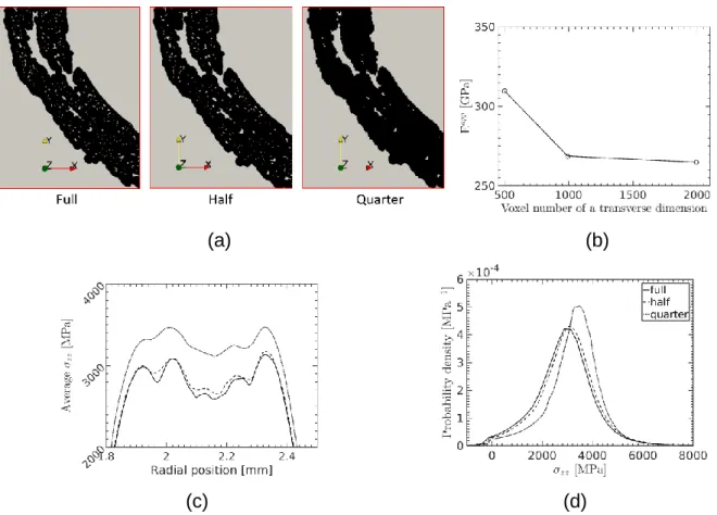
The sensitivity of the numerical solution to the image resolution has been analyzed using images with lower resolutions. The results are given in Appendix A. The full-resolution image was reduced into two lower full-resolutions (half-full-resolution and quarter resolution). The solution from the half-resolution is close to that from the full resolution, while the quarter-resolution differs significantly from the two others. This comparison shows that a half-resolution might suffice for this elastic analysis. Nevertheless, the full-resolution simulation is used in further study to reach a better accuracy of the local stress field.
3.3.2 Definitions of characteristic regions in braid architecture
To interpret the obtained stress field with respect to the complex microstructure, we define some specific regions at mesoscopic level, illustrated in Fig.9:
- Peripheral-matrix (PM): this region is located at the periphery of tows, and consists of a thick layer of CVI-deposited SiC matrix (Fig.9.a).
- Tow-core (TC): this region is defined as the non-PM region of the solid phase
(Fig.9.a). The TC region can be systematically determined as the
complementary part of the PM region in the solid phase. Both matrix and fibers can be found in this region.
- Tow border: by distinguishing the two principal dimensions of the cross section of a tow, the tow borders are defined as the boundaries of the tow along its widest dimension (Fig.9.a). Tow borders belong to PM region.
- Tow interfaces: we distinguish two types of tow interfaces (Fig.9.b), parallel interface and cross-over interface, representing the interfaces between two parallel or two cross-over tows, respectively. The former is the connection of the borders of two parallel tows, while the latter has a more complex 3D shape, since it corresponds to the zone where two crossing-over tows start to join each other.
- Triple points and V-points: the position where three tows are adjacent to each other. Note that in real braid architecture, if two parallel tows are not perfectly connected, the corresponding triple point is then decomposed into two so-called V-points (Fig.9.c).
21 (a)
(b) (c)
Fig.9 Schematic illustrating characteristic regions of braid architecture: (a) description of one single tow; (b) tow interfaces; (c) triple point.
(a) (b) (c)
Fig.10 Overview of the microstructure identification [51]: (a) transverse view, (b-c) longitudinal views. Different solid and porous phases are colored differently.
The TC and PM regions are numerically extracted in the reference image by a specific procedure based on morphological dilation/erosion operations (see [51] for more details). An illustration of the result is given in Fig.10, showing the segmentation of the braided microstructure. TC regions contain all the non-PM
22
phases (solid and micropores) and they are classified into two groups according to the tow orientations. The characteristic regions other than TC and PM will be qualitatively identified from the direct observation of the braid architecture.
In addition, in the context of the comparison between the numerical simulation results and the experimental observations, we add another region to this list: “experimentally detected cracks” (EDC) refer to the crack voxels detected in the image recorded under load, as described in section 2 [51,52].
3.3.3 Unwrapping and rescaling of stress field
To facilitate the visualization and manipulation of the stress field in the tubular composite, we first remap the fields of stress components and, in particular, of the maximum principal stress 𝜎𝑚𝑎𝑥 from the tubular geometry to a rectangular parallelepiped one. This unwrapping procedure is the same as that proposed by [67,68]. More precisely, the material point 𝑋 = (𝑟 cos 𝜃 , 𝑟 sin 𝜃 , 𝑧) in the tube is mapped to the position 𝑋𝑤 = (𝑅𝑒𝜃, 𝑟, 𝑧) . Values of the local fields at discrete positions in the unwrapped configuration are obtained by bilinear interpolation of the fields obtained from the FFT simulations. Only the region covering the composite volume is unwrapped, reducing the amount of useless voxels. Note that such an unwrapping procedure unavoidably yields a scale variation along the tube thickness, because the unwrapped circumference length becomes constant for all radii. Here, the corresponding unwrapped length is chosen to match the outer circumference 2𝜋𝑅𝑒 of the unwrapped region.
The stress field evaluated for a macroscopic applied strain of 1% has been rescaled so that the average axial stress matches the elastic limit 𝜎𝑌 (93 MPa) measured
experimentally (see stress-strain curve in Fig.1.b). The scale factor is given by 𝛼 =
𝜎𝑌/𝜎
𝑧𝑧0 , where 𝜎𝑧𝑧0 is the simulated average axial stress before rescaling, computed
over the volume of the tube (including pores where stress is zero). Doing so, the computed local stress values will provide estimates of the real stresses in the composite at the early stage of damage.
23
4. Results and discussions
4.1 Average values and probability densities of stresses
Once the stress field is rescaled to the elastic limit, some average quantities are calculated to provide a global quantification of the stress heterogeneity with respect to the different regions of the solid phase. Table 1 gives the spatial averages 𝜎𝑚𝑎𝑥 of
the maximum principal stress 𝜎𝑚𝑎𝑥 in the above defined PM, TC and EDC regions. The average stresses are similar in PM and TC regions but it is noticeably larger in the EDC regions, which confirms that the cracks are mostly initiated in stress concentration regions.
solid PM TC EDC
𝜎𝑚𝑎𝑥 (MPa) 104 100 105 139
Table 1 Average maximum principal stress 𝜎𝑚𝑎𝑥 in different regions of the solid phase.
The probability density functions of local maximal principal stresses computed at each voxel in these regions are shown in Fig.11. The curve of the TC region is similar to that of the whole solid phase, with a slightly narrower distribution. The PM region and the EDC region exhibit wider distributions, showing that the stress fields in these regions are more heterogeneous. In particular, high stresses are found within the PM region, and even higher ones in the area where cracks have been observed.
The peaks around 0 MPa in these curves suggest that some zones are unloaded in both the PM and EDC regions. This can be explained, for the PM zones, by the presence of local geometrical features, such as large pores or excrescences (see
Fig.12.a), which do not carry any load when the tube is in tension. This does not occur in the TC regions, which are under load everywhere. It is more surprising to note similarly unstressed regions in the EDC areas, where one would expect higher loads. However, one should keep in mind that the observed cracks have already undergone some propagation, even at this early loading stage. These cracks may have been initiated in highly loaded region, and their presence is highly likely to induce local stress redistributions (the origin of complex propagation), so some EDC regions might be totally unloaded before damage initiation.
24
Fig.11 Probability density functions of maximum principal stresses in different solid regions (the edge-affected zones have been excluded for this analysis).
4.2 Through-thickness heterogeneity
The stress heterogeneity through the tube thickness is here examined and discussed with respect to the experimentally detected cracks.
First, the stress field in a particular longitudinal section of the tube is shown in
Fig.12.a. The tube thickness can be schematically divided into four sublayers (L1, L2,
L3, L4), each of which representing the half of a braided layer (see Fig.12.b). Stress concentrations mostly occur around the joining zones of tows (tow interfaces), and are more pronounced at the outer tube surface than at the inner one. Conversely, unloaded areas are also observed, especially in the PM at the outer tube surface, in particular in excrescences as suggested above.
25
(a) (b)
Fig.12 (a) Longitudinal cross-section (rz plane) of the maximum principal stress field. Black lines outline the tow boundaries. The dashed line marks the radial position of the peak 4 of the upper graph of Fig.13. (b) Illustration of the braid architecture through the tube thickness, i.e. a cross-sectional slice along the direction of tows. Green dashed lines schematically indicate the peak locations of the profiles in the upper graph of Fig.13.
The volume of matrix being smaller within the TC regions than in the PM region, crack initiation is more expected to occur within the latter, as derived from the Weibull model for brittle materials (i.e. the larger the volume the higher the probability of failure). Therefore, we focus on PM region by examining the radial evolutions of the average value 𝜎𝑚𝑎𝑥 and the standard deviation 𝑠𝑡𝑑(𝜎𝑚𝑎𝑥) of local stresses ( Fig.13-upper). The two profiles are quite similar, which reveals that the highly stressed zones are always accompanied with high stress heterogeneity. For both profiles, four peaks are located at the positions where the volume fraction of macropores is small (note that peak 3 is much lower than the three other peaks). These peak locations
26
correspond to the mid-part of each half-braided layer, where the tow interfaces are located (schematically marked by the green lines in Fig.12.b).
Fig.13 Upper: radial profiles of the average maximum principal stress 𝜎̅̅̅̅̅̅̅ in the PM 𝑚𝑎𝑥 region (solid blue curve) and its standard deviation 𝑠𝑡𝑑(𝜎𝑚𝑎𝑥) (dashed blue curve),
compared to the radial profile of macroporosity volume fraction. Lower: radial profiles of surface density of the cracks detected experimentally, compared to the radial profile of the volume of peripheral matrix.
If we compare the stress distribution to the radial profile of the density of the experimentally detected cracks (red curve in Fig.13-lower), peaks 1 and 4 appear to be associated with the two peaks of the crack profile near the inner and outer tube surfaces. Yet, the crack density is clearly lower at the inner surface than at the outer one. In fact, because of the internal surface grinding, a considerable part of the PM is removed from the inner surface (see the black curve for the radial profile of PM volume in Fig.13-lower), leading to a smoother geometry at the mesoscopic scale of the tows, hence less stress fluctuations at this scale. Therefore, even though the stress average values and standard deviations are similar at peaks 1 and 4, their spatial distributions are different, which may explain different damage initiation statistics. In addition, this difference can also be attributed to the differences in the
27
crack detectability and the statistical feature of fragile fracture at the inner and outer surfaces (see (ii) and (iii) of the following paragraph).
Note also that for peaks 2 and 3 of the stress profiles, no corresponding peak is found in the crack profile, probably because of either lower stress fluctuations (peak 2) or lower average stress (peak 3) as shown in Fig.13-upper.
A more detailed analysis shows also that the two peaks of the crack profile do not exactly coincide with the peaks 1 and 4 of the stress profile in terms of radial position (as highlighted by arrows in Fig.13-lower). Some possible explanations can be proposed: (i) the experimentally detected cracks have propagated after their initiation, mostly towards the external surfaces of the tube, where more PM is present. (ii) Due to the limitations of the crack detection procedure, the cracks with small opening or extension might not be detected. These hard-to-detect cracks might mostly appear inside the tube thickness, far from tube surfaces where the cracks may be more open and thus easier to detect. (iii) According to the Weibull model, the greater the volume under consideration, the higher the probability of failure. As there is more PM at the inner and the outer tube surfaces than inside the tube thickness (see the black curve in Fig.13-lower), a higher probability for crack initiation in sublayers L1 and L4 is expected.
4.3 Stress distribution with respect to the braid architecture and the detected cracks
In order to simplify the representation of the available 3D information, we average the maximal principal stress and superimpose the detected cracks along the radial direction within each half-braided layer. In practice, this is obtained by a simple average or sum of slices in the unwrapped configuration.
Three principal zones of stress concentration are observed in the braid architecture, as highlighted by contours of different shapes in Fig.14.a: (1) cross-over interfaces, (2) separated parallel interfaces, (3) connected parallel interfaces (defined in Fig.9). In overall, these stress concentration zones are mainly located in the neighborhood of the sharp edges of macropores, within the peripheral matrix. Therefore, damage initiation should be critical in these regions. Similar conclusions can be drawn from
28
the analysis of the three other sublayers (see supplementary materials). Furthermore, the experimentally detected cracks within sublayer L4 are superimposed onto the stress projection (Fig.14.b). It is observed that almost all of them are connected to stress concentration zones, as pointed out by the arrows, even if they may also extend over much less stressed areas.
(a)
(b)
Fig.14 (a) Radial average of the maximum principal stresses in the external sublayer (L4) of the tube. Dashed lines separate the central part from the edge-affected zones. The pixels, having no solid phases in their radial paths, are colored in white. Circled areas refer to comments in the main text. (b) The same stress mapping, superimposed with the sum of the experimentally detected cracks within the sublayer L4.
This one-to-one comparison provides further arguments to the conclusion that the cracks initiate from the tow interfaces, where most peripheral matrix is located, accompanied by macropores with sharp edges. In addition, according to Weibull model, the larger the considered volume, the higher the probability of failure. The volume of matrix located in the TC region is much lower than the volume of PM, which provides an additional argument for crack initiation at tow interfaces. This
29
finding suggests that if one wants to limit crack initiation in practical applications, two improvements could be possible: (i) the tows must be stacked as regularly as possible to make them well connected at their borders; (ii) even if macropores between tows are unavoidable in fibrous preforms, the matrix should be deposited in sufficient quantity in order to reduce their sharp edges.
4.4 Influence of micropores on the stress field
In order to check the influence of micropores on the stress field, another simulation has been performed using a unit cell without micropores, i.e. the micropores are filled with solid phase. The stress field is compared to that obtained from the reference simulation (unit cell with micropores).
Fig.15 Comparison between two simulations with and without the micropores in the microstructure. Colors show the maximum principal stresses in a circumferential cross-section. The same colormap is used for both calculations.
The apparent modulus without micropores is only slightly higher than that of the reference simulation (283 GPa versus 277 GPa). In addition, the field of maximum principal stress value is compared to that of the reference simulation in Fig.15. It turns out that micropores essentially add small local fluctuations to the heterogeneous stress field induced by the macropores. The amplitude of these
30
fluctuations does not change the stress distribution at mesoscale. Stress concentrations still occur around the tow interfaces with similar intensity. This observation suggests that in the elastic regime the stress field (hence damage initiation) is mainly governed by macropores, and the presence of micropores is much less critical for damage initiation.
5. Limitations and discussions
As discussed in section 3.1, the use of the linear elastic model is reasonable for analyzing the elastic stress field, which is primarily responsible for the first crack networks inside the composite. This has been proven by the fact that almost each detected crack was connected to a stress concentration zone (Fig.14). Of course, it would have been interesting to go beyond and take into account for matrix crack propagation. However, standard non-local damage models or fracture models cannot be applied in that case. Actually, the matrix crack propagation in SiC/SiC composites is much more complex than in homogeneous materials as the crack often deviates along the fibers/matrix interface (or interphase), transferring the load from the matrix to the fibers. Although 1D modeling of such a phenomenon is now well established (see e.g. [69,70]) for the simple case of uniaxial composites submitted to tensile load, accounting for it in 3D numerical simulations with complex local loading remains an open question and a challenge for both the experimental and modeling research communities.
On the other hand, as any experimental approach, the DVC-based crack detection technique also suffered its limitation: only the cracks with an opening larger than 0.5 µm could be captured. Therefore, it is likely that some cracks are missing, whether they opened at damage initiation or after. It is also possible that some detected cracks appeared after damage initiation, when the elastic model is no more valid. Nevertheless, it seems reasonable to suppose that this experimental data spot a number of probable initiation locations significant enough to conduct this statistical study, and at mesoscopic scale. This assumption is conversely supported by the agreement between the detected cracks and the elastic stress field shown in Fig.14. Besides the undetectable cracks, some tiny micropores or their sharp edges were also not fully captured in the unit cell, as mentioned in section 3.1. These omitted
31
features might have weakened the stress concentrations related to micropores. However, this effect was believed to be not significant because the overall contribution of micropores to the fluctuation amplitudes of stress field was proven to be much smaller than that of macropores in Fig.15.
6. Conclusion
The local elastic response of a braided composite tube submitted to tensile load was modeled using the FFT method applied to the real microstructure directly obtained from a microtomographic image. A numerical test (homogeneous tube under internal pressure) demonstrated the applicability of the FFT method on tubular structures. Edge effects were quantified in order to define the size of the non-affected zone used in the quantitative analysis of the stress distribution in the braided composite tube. Using an in-house software based on the FFT method, the large scale simulation with a huge number (~6.7 billion) of voxels was completed in a short time (~21 mins). The simulated stress field was smooth and did not exhibit spurious fluctuation due to non-conformal mesh, as a direct benefit of using high-resolution images.
The stress field was analyzed and compared to the cracks detected experimentally in the same composite tube during a synchrotron tomography in situ tensile test. Through this one-to-one comparison, it was revealed that damage initiation preferentially occurs in the peripheral matrix close to the tow interfaces where sharp edges of macropores are mostly located, inducing high stress concentrations. The simulations also showed that, on the other hand, the micropores only add local fluctuations of small amplitudes to the stress distribution, which do not change the global stress heterogeneity induced by macropores.
Although only one single specimen was investigated, the information inside the unit cell was rich. The unit cell contained the whole tube circumference with three braid patterns in the axial direction. This gave us the statistics of 12 braid RVEs and a large number (~200) of microcracks detected by µCT. These could be further used to propose a statistical crack initiation criterion. Furthermore, another prospect would be to directly consider the experimentally detected cracks into the simulation, in order to examine the effect of the cracks on stress redistributions. However, when the cracks propagate in the microstructure, debonding occurs also at the fiber-matrix interface
32
(pyrocarbon interphase). The way to take into account the mechanical effects of this phenomenon in the FFT simulations remains however an open issue. Non-local damage models, namely the phase-field method [71], would be possible future work to attempt.
Acknowledgement
This work was supported by the CEA/CNRS program “Défi NEEDS Matériaux”.
Appendix A. Sensitivity of the FFT solution to image resolution
Besides the full-resolution simulation, two other simulations are also conducted over unit cells with lower resolutions (called as “half” and “quarter”, Fig.A-1.a). The two lower resolutions are numerically generated by averaging a cubic neighboring zone of 23 or 43 voxels. Every cubic neighboring zone defines a voxel of the low-resolution
unit cells, and is defined as solid or void according to the volume fraction of each phase within it. The volume fractions of porosity are 13.7%, 13.5% and 9.6% for the full, half and quarter resolutions, respectively. This indicates that the microstructure remains similar between full and half resolutions, while it is significantly modified from half to quarter resolution.
Both the macroscopic behavior (Fig.A-1.b) and the stress distributions (Fig.A-1.c and d) are compared for the three resolutions. One observes that the difference between full and half resolutions are much smaller than that between half and quarter resolutions. This suggests that the simulation with half resolution might be as accurate as that with full resolution. However, to obtain a solution the most accurate possible and also to test the capacity of our parallel implementation of FFT method, the unit cell with full resolution has been retained.
33
(a) (b)
(c) (d)
Figure A-1. (a) Parts of 2D cross sections of the three unit cells of different resolutions: full (2.6 µm/voxel), half (5.2 µm/voxel) and quarter (10.4 µm/voxel). (b) Apparent Young’s modulus versus the unit cell resolution used in the simulation. (c) Radial profile of average axial stresses in solid phase. (d) Probability density function of average axial stresses in solid phase.
Reference
[1] Katoh Y, Snead LL, Henager CH, Hasegawa A, Kohyama A, Riccardi B, et al. Current status and critical issues for development of SiC composites for fusion applications. J Nucl Mater 2007;367–370 A:659–71.
doi:10.1016/j.jnucmat.2007.03.032.
[2] Yueh K, Terrani KA. Silicon carbide composite for light water reactor fuel assembly applications. J Nucl Mater 2014;448:380–8.
doi:10.1016/j.jnucmat.2013.12.004.
34
Continuous SiC fiber, CVI SiC matrix composites for nuclear applications: Properties and irradiation effects. J Nucl Mater 2014;448:448–76.
doi:10.1016/j.jnucmat.2013.06.040.
[4] Lamon J. Properties and characteristics of SiC and SiC/SiC composites. vol. 2. Elsevier Inc.; 2012. doi:10.1016/B978-0-08-056033-5.00022-7.
[5] Deck CP, Jacobsen GM, Sheeder J, Gutierrez O, Zhang J, Stone J, et al. Characterization of SiC-SiC composites for accident tolerant fuel cladding. J Nucl Mater 2015;466:1–15. doi:10.1016/j.jnucmat.2015.08.020.
[6] Katoh Y, Snead LL, Nozawa T, Hinoki T, Kohyama A, Igawa N, et al.
Mechanical properties of chemically vapor-infiltrated silicon carbide structural composites with thin carbon interphases for fusion and advanced fission applications. Mater Trans 2005;46:527–35. doi:10.2320/matertrans.46.527. [7] Bernachy-Barbe F, Gélébart L, Bornert M, Crépin J, Sauder C.
Characterization of SiC/SiC composites damage mechanisms using Digital Image Correlation at the tow scale. Compos Part A Appl Sci Manuf
2015;68:101–9. doi:10.1016/j.compositesa.2014.09.021.
[8] Bernachy-Barbe F, Gélébart L, Bornert M, Crépin J, Sauder C. Anisotropic damage behavior of SiC/SiC composite tubes: Multiaxial testing and damage characterization. Compos Part A Appl Sci Manuf 2015;76:281–8.
doi:10.1016/j.compositesa.2015.04.022.
[9] Saucedo-Mora L, Lowe T, Zhao S, Lee PD, Mummery PM, Marrow TJ. In situ observation of mechanical damage within a SiC-SiC ceramic matrix composite. J Nucl Mater 2016;481:13–23. doi:10.1016/j.jnucmat.2016.09.007.
[10] Croom BP, Xu P, Lahoda EJ, Deck CP, Li X. Quantifying the three-dimensional damage and stress redistribution mechanisms of braided SiC/SiC composites by in situ volumetric digital image correlation. Scr Mater 2017;130:238–41. doi:10.1016/j.scriptamat.2016.12.021.
[11] Tracy JM. Multi-scale Investigation of Damage Mechanisms in SiC / SiC Ceramic Matrix Composites, PhD Thesis. University of Michigan, 2014.
35
Mater Rev 2008;53:129–81. doi:10.1179/174328008X277803.
[13] Maire E, Withers PJ. Quantitative X-ray tomography. Int Mater Rev 2014;59:1– 43. doi:10.1179/1743280413Y.0000000023.
[14] Chateau C, Gélébart L, Bornert M, Crépin J, Boller E, Sauder C, et al. In situ X-ray microtomography characterization of damage in SiCf/SiC minicomposites. Compos Sci Technol 2011;71:916–24. doi:10.1016/j.compscitech.2011.02.008. [15] Bale HA, Haboub A, Macdowell AA, Nasiatka JR, Parkinson DY, Cox BN, et al.
Real-time quantitative imaging of failure events in materials under load at temperatures above 1,600°C. Nat Mater 2013;12:40–6. doi:10.1038/nmat3497. [16] Mazars V, Caty O, Couégnat G, Bouterf A, Roux S, Denneulin S, et al.
Damage investigation and modeling of 3D woven ceramic matrix composites from X-ray tomography in-situ tensile tests. Acta Mater 2017;140:130–9. doi:10.1016/j.actamat.2017.08.034.
[17] Walker SM, Schwyn DA, Mokso R, Wicklein M, Müller T, Doube M, et al. In Vivo Time-Resolved Microtomography Reveals the Mechanics of the Blowfly Flight Motor. PLoS Biol 2014;12. doi:10.1371/journal.pbio.1001823.
[18] Schöberl J. An advancing front 2D/3D-mesh generator based on abstract rules. Comput Vis Sci 1997;1:41–52. doi:10.1007/s007910050004.
[19] Keyak JH, Meagher JM, Skinner HB, Mote CD. Automated three-dimensional finite element modelling of bone: a new method. J Biomed Eng 1990;12:389– 97. doi:10.1016/0141-5425(90)90022-F.
[20] Kim HJ, Swan CC. Voxel-based meshing and unit-cell analysis of textile composites. Int J Numer Methods Eng 2003;56:977–1006.
doi:10.1002/nme.594.
[21] Liehr F, Preusser T, Rumpf M, Sauter S, Schwen LO. Composite finite elements for 3D image based computing. Comput Vis Sci 2009;12:171–88. doi:10.1007/s00791-008-0093-1.
[22] Strouboulis T, Copps K, Babuška I. The generalized finite element method. Comput Methods Appl Mech Eng 2001;190:4081–193. doi:10.1016/S0045-7825(01)00188-8.
36
[23] Sukumar N, Chopp DL, Moës N, Belytschko T. Modeling holes and inclusions by level sets in the extended finite-element method. Comput Methods Appl Mech Eng 2001;190:6183–200. doi:10.1016/S0045-7825(01)00215-8. [24] Becker R, Hansbo P, Stenberg R. A finite element method for domain
decomposition with non-matching grids. ESAIM Math Model Numer Anal 2003;37:209–25. doi:10.1051/m2an.
[25] Butrylo B, Musy F, Nicolas L, Perrussel R, Scorretti R, Vollaire C. A survey of parallel solvers for the finite element method in computational electromagnetics. COMPEL - Int J Comput Math Electr Electron Eng 2004;23:531–46.
doi:10.1108/03321640410510721.
[26] Zhu Y, Sifakis E, Teran J, Brandt A. An efficient multigrid method for the simulation of high-resolution elastic solids. ACM Trans Graph 2010;29:1–18. doi:10.1145/1731047.1731054.
[27] Baker AH, Gamblin T, Schulz M, Yang UM. Challenges of scaling algebraic multigrid across modern multicore architectures. Proc - 25th IEEE Int Parallel Distrib Process Symp IPDPS 2011 2011:275–86. doi:10.1109/IPDPS.2011.35. [28] Sahni O, Zhou M, Shephard MS, Jansen KE. Scalable implicit finite element
solver for massively parallel processing with demonstration to 160K cores. Proc Conf High Perform Comput Networking, Storage Anal - SC ’09 2009:1. doi:10.1145/1654059.1654129.
[29] Tian R, Wang C. Large-Scale Simulation of Ductile Fracture Process of Microstructured Materials. Prog Nucl Sci Technol 2011;2:24–9.
[30] Mosby M, Matous K. Universal Meshes: A new paradigm for computing with nonconforming triangulations. Int J Numer Methods Eng 2015:748–65. doi:10.1002/nme.
[31] Mosby M, Matous K. Computational homogenization at extreme scales. Extrem Mech Lett 2016;6:68–74. doi:10.1016/j.eml.2015.12.009.
[32] Moulinec H, Suquet P. A FFT-based numerical method for computing mechanical properties of composite materials from images of their