A Novel (3T-1R) Redundant Parallel Mechanism with Large Operational Workspace and Rotational Capability

HAL Id: lirmm-00906223

https://hal-lirmm.ccsd.cnrs.fr/lirmm-00906223

Submitted on 19 Nov 2013

HAL is a multi-disciplinary open access

archive for the deposit and dissemination of

sci-entific research documents, whether they are

pub-lished or not. The documents may come from

teaching and research institutions in France or

abroad, or from public or private research centers.

L’archive ouverte pluridisciplinaire HAL, est

destinée au dépôt et à la diffusion de documents

scientifiques de niveau recherche, publiés ou non,

émanant des établissements d’enseignement et de

recherche français ou étrangers, des laboratoires

publics ou privés.

Large Operational Workspace and Rotational Capability

Samah Aref Shayya, Sébastien Krut, Olivier Company, Cédric Baradat,

François Pierrot

To cite this version:

Samah Aref Shayya, Sébastien Krut, Olivier Company, Cédric Baradat, François Pierrot.

A

Novel (3T-1R) Redundant Parallel Mechanism with Large Operational Workspace and

Rota-tional Capability. IROS: Intelligent Robots and Systems, Nov 2013, Tokyo, Japan. pp.436-443,

�10.1109/IROS.2013.6696388�. �lirmm-00906223�



Abstract— This paper presents a novel 4 dofs (3T-1R (1)₎

parallel redundant mechanism, with its complete study regarding inverse and direct geometric models (IGM and DGM), as well as singularity and workspace analysis. The robot is capable of performing a half-turn about the z axis (a complete turn would be theoretically possible if it were not for possible unavoidable inter-collisions in the practical case), and having all of its prismatic actuators along one direction, enables it to have an independent x motion - only limited by the stroke of the prismatic actuators. The mechanism is characterized by elevated dynamical capabilities having its actuators at base. Moreover, the performance of the robot is evaluated considering isotropy in velocity and forces.

I. INTRODUCTION

Parallel mechanisms have been known for their increased rigidity, better accuracy, higher load and dynamical capacities as compared to their competent serial mechanisms. Unfortunately, these mechanisms are not without their own drawbacks such as limited workspace and presence of the so referred to as parallel singularities, in addition to the usual serial type singularities. However, the advantages of such mechanisms, are quite sufficient to be the motive behind the increasingly interest in these mechanisms, in which they have been under extensive research in the last decades.

At their infancy, most of the parallel mechanisms that have been studied are of 6 dofs (3T-3R) known as the Gough-Stewart platforms or “hexapods” which appeared in the early 1950’s and 1960’s. Later on, parallel mechanisms with lower mobility (2) _{have been studied and investigated. In}

fact, for most industrial applications-such as machining, laser cutting, pick-and-place applications- 6 dofs are too much. Thus studies have been conducted regarding the synthesis of 3 dofs (3T), 4 dofs (3T-1R) and 5 dofs (3T-2R) parallel mechanisms.

* This work has been supported partially by the French National Research Agency within the ARROW project (ANR 2011 BS3 006 01) and by Tecnalia France.

Samah Shayya (corresponding author) and Cédric Baradat are with Tecnalia France – MIBI Building, 672 Rue du Mas de Verchant, 34000 Montpellier, France. E-mails: samah.shayya/cedric.baradat@tecnalia.com

Sébastien Krut, Olivier Company, and François Pierrot are with the Montpellier Laboratory of Informatics, Robotics, and Microelectronics (LIRMM in French), a cross-faculty research entity of the Montpellier University of Sciences and Technologies (UM2) and the French National Center for Scientific Research (CNRS), 161 rue Ada, 34095 Montpellier, France. E-mails: krut/company/francois.pierrot@lirmm.fr

(1) _{3T-1R: Three-translational degrees of freedom and one rotational}

degree of freedom.

(2) _{i.e. number of dofs<6}

In fact, regarding some tasks 4 dofs (3T-1R) parallel mechanisms are sufficient. In others, where another rotation is required it can be provided either by the table or by an additional actuator in series with the parallel mechanism (forming a hybrid mechanism). Many 3T-1R parallel mechanisms exist in literature such as the famous Delta robot [1] (with the R-U-P-U (3) _{chain), the Kanuk [2], the SMG in}

[3], the H4 in [4], the I4 in [5], the Par4 in [6] with its industrialized version Adept Quattro [7] (fastest industrial pick-and-place robot). Also, an interesting family of fully-isotropic parallel 4 dofs (3T-1R) mechanisms, in addition to decoupled mechanisms, has been synthesized in [8]. In [8], there is an elaborated referencing to other 4 dofs mechanisms.

However, these and other existing mechanisms have some inconveniences. For example, in the case of Delta with a huge workspace (even much larger with linear Delta), the presence of the RUPU chain connecting the base to the platform to supply the rotational dof is a weak element reducing the workspace. Others present problems of singularities, limitation of workspace (and particularly) in rotational capability, complexity of obtaining analytical expressions for the direct geometric model, and /or the use of transmission systems with the articulated platform in the case [4-7]. Actually, the use of transmission systems such as gears or cable and pulleys in the platform, will impact accuracy and repeatability of the robot. The mechanisms in [8], despite their interesting isotropic property, have a limited workspace (having the prismatic actuators in different directions), and are complex from manufacturability and industrialization point of view.

In this paper we present, a 4 dofs (3T-1R) parallel mechanism with actuation redundancy (two degrees of redundancy) that responds to the major requirements: large operational workspace, high rotational capability, absence of singularities, design simplicity, high rigidity, and high dynamical capabilities with analytical expressions for the inverse and direct geometric models. Such mechanism is intended to be used as 4 dofs (3T-1R) module in a 5 dofs (3T-2R) parallel kinematic machine where the 5th _{dof (2}nd

rotational dof) is provided by a turntable according to left-hand right-left-hand paradigm. Such machine can be used in many industrial applications requiring 5 dofs such as laser cutting, five-faces machining, etc...

(3) _{R, U, and P: correspond to rotational, universal, and prismatic joints.}

Bold face letter means actuated, and underlined letter means the joint position is measured.

A Novel (3T-1R) Redundant Parallel Mechanism with Large

Operational Workspace and Rotational Capability*

The paper introduces the mechanism in section II and its geometrical elements. Then sections III and IV detail the inverse and direct geometric models respectively. Section V presents the singularity and workspace analysis of this mechanism. The paper ends with section VI giving the conclusions.

II. THE NEW 4DOFS (3T-1R)MECHANISM

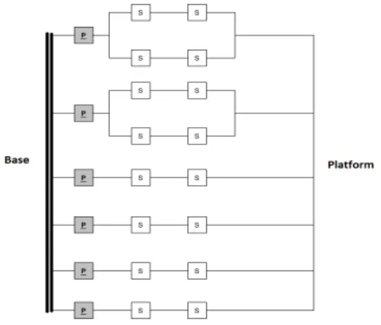
The graph diagram of the four dofs (3T-1R) parallel mechanism we propose is shown in fig.1 with its CAD drawing in fig. 2 and fig.3. The platform, its dimensions and the platform connection points labeling are clarified in fig. 4. Note that this mechanism has been chosen among other synthesized mechanisms with same number of actuators and dofs, and after several studies. This synthesis procedure will not be discussed here for brevity.

The robot consists of six actuators along the same direction (x-axis) and can perform four motions x, y, z and Θ (rotation about z-axis). The robot is redundant (having two extra actuators). It is quite clear that this robot can move along x independently of the other motions y, z and Θ. This motion along x is only limited by the available stroke for the prismatic actuators.

The principle of functioning of this mechanism is straight forward. The role of parallelograms in chains (III) and (IV) is to constraint the platform rotation about any axis that is perpendicular to the z axis direction of the base frame. These two parallelogram arms cooperate with the other four simple arms to position the TCP and control the platform orientation about the axis parallel to the z axis of the base frame.

Figure 1. Graph diagram of the mechanism. P: prismatic joint, S: spherical joint. Gray box means actuated, while white box means passive.

The underlining signifies that the joint position is being measured. It is worth mentioning that the mechanism is theoretically capable of complete rotation, but in practical case there might be possibility of unavoidable inter-collisions, so we can guarantee practically a half-turn (



    



90 ; 90



) free of inter-collisions which is considered by itself sufficient (maximum required rotation range in real applications). Moreover, the spherical joints can be practically replaced by

three revolute joints as to overcome known limitations of the commercial spherical joints regarding rotation capabilities.

We define the different geometrical elements of the mechanism before establishing its models and Jacobians. The following notations are used:

 L i_i ( 1...6) is the length of the ith _{arm of extremities}

i

A

and B_i.

 Ai , B ii ( 1...6) are the connection points of the arm

i i

A B (ith _{arm) as shown in the figures 3 and 4. In case of}

parallelogram arm, they are along the mid-axis of the parallelogram.

Figure 2. Simplified CAD drawing of the mechanism for clarification purpose only. The rotation of the platform is greater than 90°. The x, y and

z directions of the base frame are shown in the figure.

Figure 3. Frontal view of the robot. The pose illustrated is for ϴ=0°. The x, y and z directions of the base frame are shown in the figure.

Figure 4. Platform and its principal dimensions. The x, y and z directions of the moving frame connected to the platform are shown on the figure.  ui (i1...6) is the unit vector along the direction of the

 ni (i1...6) is the unit vector along the vector A Bi i.







T

i  pxi pyi pzi

p is the vector directed from P (the TCP) to B_i expressed in the base frame of the robot.







T ( 1...6) m m m i  pxi pyi pzi i m p is the vector

directed from P (the TCP) to B_i expressed in moving frame of the platform.

 e_x ,e_y ,e are the unit vectors along the x, y and z axis _z

of the base frame respectively.







T

( 1...6)

i i i

x y z i are the coordinates of the point i

A (note that y_i and z_i are constant).







T

x y z



p is the vector OP where O is the origin of the base frame.

  is the rotational angle.







T

x y z 



x is the pose of the robot.







T

1 6

q q



q is the joints displacement vector of linear actuators. 



1



T 6 r r x x  r

X is the vector containing the values of xi (i1...6) corresponding to the assumed zero

extension or displacement of the linear actuators (i.e. for which we consider q0); it is constant vector just marking the origins of joints’ displacements meaning that q_i  x_i x_ir, i1...6 or



 

T



T

1 6 1r 6r

x x x x

 

q . One can assume

joints’ displacements origins to be confounded with x-axis origin i.e. at X_r 0 and hence q



x₁ x₆



T.

 z 0 Rot ( ) 0 0 0 1 c s s c          _{  }    

R is the rotational matrix of

the platform frame with respect to the fixed base frame where c_ cos( ) and s_ sin( ) .

 Define ξ the geometric parameters vector with its g

elements being Li, yi ,zi ,xir with i1...6.  Note that | 1 3 |

m m

x z

d p p which is shown in fig. 4.  Also note that || 1 5|| | 1 5 |

m m

z z

a B B  p p which is shown also in fig. 4.

We assume the following in our study:  B1B2,B3B4 ,B5B6  L1  L2 L5 L6 , L3L4  y1    y5 y2 y6 , y3 y4  z1z2z5 z6 , z3z40  | 1 3| | ( 1 3 ) | m m z z

z z  p p : This is a necessary condition to have a functioning mechanism (in order to be able to control the z position of the TCP).

The coordinates of B_i are expressed in the base frame as





T

i xbi ybi zbi

B .

III. THE INVERSE GEOMETRIC MODEL (IGM) The inverse geometric model (IGM) for parallel robots is usually easy to determine and our mechanism is not an exception of this idea. To establish the IGM we suppose that we have the robot’s pose x and all the geometric parametersξ , and then we need to calculate the joints _g variables qIGM (x, ξ . Note that: _g)



 

T



T

x y z  

 

x p (1)

Then, we can get the coordinates of B_i as follows:

, 1...6 i  i  i m B p R p (2) Substituting _im p and R, we get: , 1...6 m m xi yi bi m m i bi xi yi m bi _zi x p y p c p s x y s p c z _{z p} i          _{ }                _{ }     B (3)

The term _pim _{is the vector coordinates of point}

i

B in the platform frame which is known. Now, to get the coordinates of A_i we need to utilize the following equation:

2 2 , 1...6 i i Li  i A B (4) Equation (4) gives: 2 2 2 ( ) ( ) , 1...6 i xbi Li bi i bi zi x    y y  z   i (5)

As long as the term within the square root is positive, two real solutions for each x_i are possible. The choice depends on the assembly mode we choose. In our case, we will choose to have the actuator to be before the platform, meaning: 2 2 2 ) ( ( ) i bi i bi i bi i x  x L  y y  z z (6) Substituting the value ofx_bi, we get:

2 2 2 ) ) ( ( m m i xi yi m m m i xi yi i zi i x c p s s p c x p L y p y z p z                (7)

Now, to get q we need to assume a certain reference for the linear actuators, i.e. a set of values of x ii ( 1...6) for which

we consider q0. Call this referenceX_r 



x_1r x_6r



T

as we previously said in section (II), then:



1 6

 

1 6



T T r r x x x x   q (8)

1 1 6 2 2 2 1 1 6 6 1 1 1 1 1 6 6 6 6 6 6 2 2 2 ( ( ( ) ) ( ) ) m m r x y m m r x y m m m x y z m m m x y z c p s c p s s p c y z p s p c y x x p x x p L y p z L y p z p z                  _     _{    }                          q (9)

Hence, the IGM is established. Note that regardingX_r, one can take it as zero, assuming that qi0 when the

corresponding x_i 0 or it can be chosen for example by assuming that q0 when x0 and thus in this case, we

have



_{1 6}

 

T _{1 6}



T at r r x x x x    x r X 0 . IV. THE DIRECT GEOMETRIC MODEL (DGM) Unlike serial robots, the direct geometric model (DGM) of a parallel manipulator is most often difficult to be determined analytically. However, with this mechanism it is easy to establish its DGM. Supposing that we have q we need to get xDGM ( ,q ξ_g)IGM ( ,-1 q ξ_g). We emphasize that there is no unique way to establish the DGM in our case, the robot being redundant. Here, we present one possible way. Suppose we know q then all points’ coordinates Ai(i1...6) are known. Let us get points B1

first. We have the following equations (we will be very brief due to space limitation):

2 2 2 2 1 1 1 1 1 1 1 (x_b x) (y_b y) (z_b z) L (10) 2 2 2 2 1 2 2 1 1 2 2 (x_b x ) (y_b y ) (z_b z ) L (11) 5 5 2 2 5 5 2 5 5 5 2 (x_b x) (y_b y ) (z_b z ) L (12) But at all times, we have:

5 1 5 1 5 1 1 5|| | 5 1 5 1 , , || | | | b b b b b b m m z z z z p x x y y z z a a p p p              B B (13)

Then substituting (13) in (12), we get:

2 2

5 5

2 2

1 5 1 1 5

(x_b x ) (y_b y ) (z_b (z a)) L (14) Subtracting (11) from (10), we get the equation of the plane

1

(pl) (containing the intersection circle of the two spheres). Subtracting (14) from (10), we get plane (pl₂) in which the intersection circle between the two corresponding spheres is present.

Now, we have two planes that intersect at a line(ln₁)(pl₁) (pl₂) whose parametric equations can be easily derived. To get the point B₁ of coordinates B₁, we need to substitute the parametric equations of (ln1) in one

of the equations (10), (11) or (12). In general, we get two possible solutions call them 1

1 s B and 2 1 s B . Substituting the values of B₁ in (13), we get also two possible solutions for

the coordinates of B₅, call them 1 5 s B and 2 5 s B , respectively. Now consider the equations, below to get coordinatesB₃:

2 2 2 2 3 3 3 3 3 3 3 (x_b x ) (y_b y) (z_b z ) L (15) 4 4 2 2 3 4 2 3 3 4 2 (x_b x) (y_b y ) (z_b z ) L (16) Note that z component of B₃ can be directly calculated using the following relation:

1 3  3 1 ( 3  3 )

m m

B B p p R p p (17)

But we have only one rotation which is about e meaning: _z

, 1...6 m zi zi p p  i (18) Then: 3 1 3 1 m m b b z z z z p p (19)

Since we have now z_b3 (two possible values), the system of equations formed by (15) and (16) reduces to be system of equations of two variables, namely x_b3 and y_b3. The solution is simply the intersection of these two circles described in (15) and (16). For each value of z_b3, we obtain two points, thus four possible coordinates in total, call them

11 3 s B , 12 3 s B (corresponding to 1 3 s b z ), 21 3 s B and 22 3 s B corresponding to 2 3 s b z .

Recall that B₁B₂,B₃B₄,B₅B₆. At the end, we have a set of four possible solutions, call it . This set is:





















1 2 3 4 1 1 11 1 1 12 1 1 2 3 2 1 2 3 2 2 21 2 2 22 3 1 2 3 4 1 2 3 , , , , , , , , , , , , ,    _{ }      s s s s s s s s s s s s S S S S S B B B S B B B S B B B S B B B (20)

Then, the solution is S and such that we have the relation below satisfied (implied from (6)):

, 1...6

i bi

x x  i (21)

Now having determined the coordinates B_i for all points B_i, we can determine the pose by taking only the x and y components of the vector B B_{1 3} , call them _x and _y respectively. Knowing these latter two components we can determine



  



 

;



using arctan 2 ( _y, _x). Then we have the rotational matrix R, and the position of the TCP is calculated by:





T

 

1 1 1 1 , Rotz x y z       m  p B p B R p R (22)

The pose x



x y z 



T is calculated and hence the DGM is analytically established, for this new mechanism.

V. SINGULARITY AND WORKSPACE ANALYSIS An important step in the study of a parallel mechanism is investigating the presence of singularities. To do this, we need to establish the Jacobian J or the inverse Jacobian J_m For redundant parallel mechanisms, the inverse Jacobian is straight forward whereas J requires in case of redundancy the use of pseudo-inversion procedure.

Let us consider the velocity and angular velocity of the TCP to be denoted by v and w , respectively. These are given in our case as follows (4)_:





T d x y z dt   p v p (23) z w   z  z w e e (24)

Then, we define our reduced 4x1 twist vector t as follows:





T





T x y z z v v v w x y z    t (25)

Then inverse Jacobian J_m relates the joint velocity vector q to the twist vector t by:

 m

q J t (26)

To find the above relation, we need to differentiate

2 2

constant i

i i L 

A B with respect to time which gives the following expression: , 1...6 i i i i i i A  i i B  i A  i B  i A B v A B v n v n v (27) The terms i A v and i B

v are the linear velocities of the points i

A and B_i respectively and are calculated using the following two equations:

, 1...6 i qi iqi  i A x v u e (28) ( ) , 1...6 i i i i i              B z z v v w p v e p v p e (29) Substituting the latter two equations in (27) and writing the 6 equations in matrix form we get:



q x

J q J t (30)

The matrices J and _q J_x are given as follows:

diag ( ) diag ( ) diag ( ) dim ( ) 6 6 i i i i nx      q x q J n u n e J (31) 6 T T 1 1 1 T 6 T 6 ( ) ) 6 4 ( ) , dim (             _     z x x z p e J p e n n J n n (32)

Then, when the inverse of J exists, the inverse Jacobian _q

matrix J_m is given by the following equality:

1 , dim( ) 6 4     m q x m J J J J (33)

It is important to note that in what follows, we will be talking about the yz region rather than talking about the xyz region, simply due to the fact that x motion can be provided independently of the other y, z and ϴ motions. We do not talk about accessibility region regarding ϴ since we mean by the yz region with full rotational capability (that is practically guaranteed), the region where the robot can perform half-turn (practically we are interested in half-turn rather than full rotation because 180° is the maximally needed rotation range on

(4) _f df dt

 where t is time and f is a function of time.

one hand and on the other hand in practice we would have unavoidable inter-collisions in case of complete rotation as discussed earlier in section (II) but this has nothing to do with singularity).

A. Series Type Singularities

The series type singularities correspond to the case where the twist t0, but the joint velocity is non-zero i.e. q0. This situation is present when the square diagonal matrix

q

J is non-invertible. This is expressed mathematically as:





0

0

det (J_q) 0  i  1, 2 ,..., 6 ; n_i e_x0 (34) Relation (34) simply implies that we have serial type singularity when one of the arms is perpendicular to the x axis, meaning when the arm is in the yz plane. If the pose that might lead to such a case exists (i.e. it is geometrically accessible), such pose will obviously be at the envelope of the yz geometrically accessible workspace, because in this case the corresponding point

0

i

B will belong to a circle of center 0 i A and radius 0 i

L in the plane parallel to the yz plane, and there is no doubt that in the geometrically accessible yz region of the TCP, the point

0

i

B for sure cannot be except on this circle and not outside it or within it. This means since the TCP is at constant distance from

0

i

B , it is necessary that the TCP is in this case at the boundary of the yz geometrically accessible region.

B. Parallel Type Singularities

Parallel type singularities occur when the joint velocity is null i.e. q0, while the platform is capable of infinitesimal motion i.e. t0 . This means that matrix J_x is rank deficient. In our case, J_x is singular when its rank is less than 4. We know that the rank of the matrix will not change if we do linear operations on the matrix columns or rows. In

our case, we will add



T T



T

1 ( 1 z) 6 ( 1 z)

n p e n p e to

the 4th _{column of}

x

J which is a linear combination of the first three columns. We will call the new matrix N . Note that: B₁B₂ , B₃B₄ and B₅B₆. Then the new matrix is: T 1 T 2 T T 3 T T 4 4 T 5 T 3 6 0 0 ( ) ( ) 0 0        _{ }                 z z n n n n r e N n n r e n n (35)

The vector r is given by:

1 3 1 4

 

r B B B B (36)

Consider the matrix M defined by:





T

 1 2 5 6

The vectors which form the matrix M form the basis of two non-parallel planes which are plane pl A A B( _{1 2 1}) and plane

5 6 5

( )

pl A A B since |z₁z₅| B B| | _{1 5} | (refer to the figures at beginning). This obviously means that:







1 2 5 6



_





_

span n,n ,n ,n span e_x,e_y,e_z (38) Relation (38) implies that M is of rank 3 since the span of its row vectors is equal to the span of the basis of 3_{. Hence,}

for N (and thus J_x) to be full rank, it is necessary and sufficient that at least T

3 (  z) 0 n r e or T 4 (  z)0 n r e . However, having ₃T ₄T (  z) (  z)0 n r e n r e implies that all the vectors n₃, n₄, r and e are in the same vertical _z

plane (i.e. containing e ), which is only possible when these _z

vectors are in a plane parallel to the yz plane, since we

always have , 1...6

i

i b

xx  i due to relation (6). Having the vectors n₃ and n₄ in plane parallel to yz plane, simply means that we also have –if pose is geometrically accessible-serial type singularity which cannot occur except at the boundary of the yz accessible region as we explained earlier in the previous section.

Hence, N (equivalently J_x) is always of full rank within the yz geometrically accessible region, and if it is to be rank deficient, this would not happen except at boundary of this region.

C. Conclusion on Singularity Analysis

Hence, within the geometrically accessible yz region excluding its boundary, we can guarantee always that there are neither serial nor parallel type singularities. This is due to the fact that these singularities if were to occur, are not possible except at boundary of this region.

D. Workspace Analysis

As we mentioned earlier, the workspace analysis can be limited to investigating the yz region that allows for half-turn and where the value of the chosen performance index is within the acceptable range.

There are several indices in literature that might be used to evaluate the robot’s performance [9-11] and each has its own problems which is not our concern here. However, in our case, we are interested in isotropic performance of the robot regarding operational velocity and static operational force. The robot under study being redundant the singular values of the inverse Jacobian matrix are no longer significant regarding this aspect and so is the condition number based on the ratio of largest singular value to the minimal one, as discussed in [12]. So, in our study and evaluation of workspace, we defined the following index:

min w, w wl wl v f FVI v f    _{ }   (39)

The terms v_w and f_w are the worst speed and the worst force (5) _{respectively, whereas}

wl

v and f_wl are the desired lower bounds for the worst speed and worst force respectively. Actually, v_w is nothing except the largest isotropic speed (radius of the largest sphere included in the zonotope of the operational velocities), and f_w is similarly the largest isotropic force (radius of largest sphere included in operational force zonotope considering that joint torque vector satisfies

 

T T

null

  

 Jm  τ 0 (refer to footnote

(5)_{)). In}

our case, we have chosen vwl q_max 2 and fwl max 2.

The terms q_max and _max are respectively the maximum speed and maximum force for the linear actuator (all actuators are considered identical).

Since we have mixed degrees of freedom (translation and rotation), it is mandatory to homogenize J_m before evaluating the index at each pose. For this purpose, we use a suitable weighing matrix as suggested in [13].

Our weighing matrix is W diag 1,1,1,



d 2



. The term

d is the distance shown in fig. 4. Then, consider the homogeneous inverse Jacobian matrix  1

mw m

J J W and its pseudo-inverseJ_w. We then have:

1...6 max ma 6 x 1... 1 min || || 1 min || || i i i i w w v q f         _ _     _{ }      _{ }     mwr wc j j (40) The terms i mwr j and i wc

j mean the ith _{row vector of matrix}

mw

J and ith _{column vector of the matrix}

w

J . The proof of (40) is similar to the proof of the dynamical index introduced in [14].

So, in what follows we established the yz region with null orientation (  0 ) and the yz region with rotational range of 180° (



    



90 ; 90



), and where FVI1. Regarding the case of yz region with rotational capacity, we have evaluated FVI for a set of different rotational angles particularly (-90° , -60°, -45°, -30°, 0°, 30° , 45°, 60°, 90°) for the purpose of reducing computation time and we assumed the worst value of this index for the corresponding

( , )y z position (in this case the minimal value of FVI). Note although the mechanism is capable of full turn

(5)

w

f is calculated considering minimum norm torque vector solution

of _ T m

f J τ i.e. considering the joint torques vector τ satisfying

 

T

T

null

  

 Jm  τ 0 and thus having:

T  T  * m J f τ J f with  * m J J the

pseudo-inverse of J and f the operational force vector. Note to have m

physical significance and consistency of f , the matrix w J must be m

theoretically, we evaluated performance on



90 ; 90





     which we usually need for most

applications (maximum required range for most applications) and since for complete turn we might have practically unavoidable inter-collisions as previously mentioned. For this study, we used the following optimized parameters:

1 1 3 3 3 1 1.25 , 1.0926 , 0.375 , 0.4602 0.3 , 0 , 0.1126 , 0.2 L m L m y m y m z m z m d m a m          

The other parameters can be determined using the relations we have already given at the end of section II. The figures below show boundary plots of yz region accessible with

0

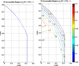
   and with full range of  satisfyingFVI1. Also, we provided a contour plot to show how the value of the index changes as function of ( , )y z . Note that the yz regions in both cases are symmetric with respect to the y and z axes. So, we have shown in the figures the boundaries and contour plots of the yz regions belonging to the first quadrant for clarity purpose only. These plots show that the yz region with and without orientation is large, especially when we consider the available space between its slider guides, which is quite interesting (in the evaluation of the workspace we posed the condition y₁d 2  y y₂ d 2 in order to avoid collisions with the sliders guides).

To have better insight of the index variation within the workspace, we have provided a table (table I) presenting the value of area in case of null orientation and full orientation capacity (between -90° and +90°), together with mean value and standard deviation of the index over the corresponding yz region. The small standard deviation as compared to the corresponding mean value shows that the index variation over the yz region is relatively low which is advantageous.

Figure 5. On the left we show the boundary of yz region accessible with null orientation. On the right we show the contour plot showing the variation of the FVI index as function of the position (y, z) in the case of null orientation. These have been shown on the quarter of the workspace

due to symmetry with respect to the y-axis and z-axis.

Figure 6. Boundary of the accessible yz region with full orientation capability (between -90° and +90°). It has been shown on the quarter of the

workspace due to symmetry with respect to the y-axis and z-axis.

Figure 7. Contour plot showing the variation of the index FVI as function of the position (y, z) and for full orientation capacity (the value shown at each position is the worst value (smallest) of the index among the different

angles tested between -90° and 90°). It has been shown on the quarter of the workspace due to symmetry with respect to the y-axis and z-axis.

TABLE I. RESULTS OF THE WORKSPACE ANALYSIS REGARDING AREA OF THE ACCESSIBLE YZ REGION AND THE VARIATION OF THE INDEX OF PERFORMANCE FVI DESCRIBED BY THE VALUE AND STANDARD DEVIATION.

Case Estimated Area (m2₎ Mean Value of FVI Standard Deviation of FVI Null Orientation (ϴ=0°) 0.79 1.21 0.08 Full rotational capacity (range of ϴ: -90° to +90°) 0.69 1.14 0.07

VI. CONCLUSIONS AND FURTHER WORK

In this paper, we have presented a new 4 dofs (3T-1R) parallel redundant mechanism. It has 6 actuators for 4 dofs; the interest in this actuation redundancy is eliminating

singularities and improving performance. We also have established both the inverse and direct geometric models, and presented a complete analysis of the Jacobians and the singularities. Moreover, we have calculated the different workspaces and presented a new singularity index “FVI ”

which is suitable for redundant and non-redundant robots as well. In case, of heterogeneous Jacobian (case of mixed dofs), a homogenization is needed prior to evaluation of the index for a certain pose.

The workspace of this mechanism along x direction is independent of the other motions and only limited by the available stroke of the linear actuators, which is one of its major advantages. The yz accessible regions are large in both cases with and without orientation, especially when compared to the space between its slider guides. The mechanism is particularly interesting having the capability to perform a half-turn (which is large and maximum required rotation capability for most applications), knowing that a complete rotation would be possible if it had not been for the possibility of unavoidable inter-collisions in practical situation.

Furthermore, another advantage of this robot is having its workspace symmetric with respect to xz and yz planes, free of collisions and also convex. The latter property, namely convexity, is very advantageous regarding trajectory planning; any two points in the workspace can be connected by a straight line trajectory.

Besides, having the arms connected to platform and actuators via spherical joints, puts these arms under tension/compression forces making it easier to model deformation and compensate for it.

In brief the simplicity of the design, the actuation redundancy, the actuation at base, and the high stiffness of the mechanism contribute to the high dynamical performance capabilities (regarding pay-load, acceleration and velocity) as well as to its enhanced performance regarding accuracy and precision.

Regarding the future work, it is important to optimize the design further in the sense of implementing it and producing a prototype on which real performance can be evaluated.

REFERENCES

[1] R. Clavel, “Une nouvelle structure de manipulateur parallèle pour la robotique légère », APII, 23(6), 1985, pp. 371-386.

[2] Rolland L., “The Manta and the Kanuk: Novel 4 dof parallel mechanism for industrial handling”, in Proc. of ASME Dynamic Systems and Control Division IMECE’99 Conference, Nashville, USA, November 14-19, 1999, vol. 67, pp. 831-844.

[3] J. Angeles, S. Caro, W. Khan, A. Morozov, « The kinetostatic design of an innovative Schonflies-motion generator », Proceedings of the Institution of Mechanical Engineers, Part C: Journal of Mechanical Engineering Science 220 (7) (2006) 935–943.

[4] F. Pierrot, O. Company, H4: a new family of 4-dof parallel robots, In: Proc. of the IEEE/ASME Int. Conf. on Advanced Intelligent Mechatronics, Atlanta, USA, 1999, pp. 508–513.

[5] S. Krut, O. Company, M. Benoit, H. Ota, and F. Pierrot, “I4: A new parallel mechanism for Scara motions,” in Proc. of the 2003 Int. Conf.

on Robotics and Automation, Taipei, Taiwan, September 2003, pp. 1875–1880.

[6] V. Nabat, O. COMPANY, S. KRUT, M. Rodriguez, and F. PIERROT, “Par4: very high speed parallel robot for pick-and-place”, in Proc. IEEE International Conference on Intelligent Robots and Systems (IROS’05), Edmonton, Alberta, Canada, August 2005. [7] F. Pierrot, V. Nabat, O. Company, S. Krut, “From Par4 to Adept

Quattro”, in Proc. Robotic Systems for Handling and Assembly - 3rd International Colloquium of the Collaborative Research Center SFB 562, Braunschweig, Germany, (2008).

[8] Grigore Gogu, “Structural synthesis of fully-isotropic parallel robots with Schonflies motions via theory of linear transformations and evolutionary morphology”, European Journal of Mechanics A/Solids 26 (2007) 242-269.

[9] J. K. Salisbury and J. J. Craig, “Articulated hands: force control and kinematic issues”, International Journal of Robotics Research, Vol. 1, no. 1, pp. 4-17, 1982.

[10] T. Yoshikawa, “Manipulability of robotic mechanisms”, International Journal of Robotics Research, Vol. 4, no. 2, pp. 3-9, 1985.

[11] C. Gosselin and J. Angeles, “Global performance index for the kinematic optimization of robotic manipulators”, Transaction of the ASME, Journal of Mechanical Design, Vol. 113, no. 3, pp. 220-226, 1991.

[12] S. Krut, “Contribution à l’étude des robots parallèles légers, 3R-1R et 3T-2R, à forts débattements angulaires », Ph.D Thesis, Université Montpellier II, Novembre 13, 2003.

[13] L. Stocco, S. E. Salcudean and F. Sassani, “Matrix Normalization for Optimal Robot Design”, in Proc. of IEEE ICRA, Leuven, Belgium, May 16-21, 1998.

[14] David Corbel, Marc Gouttefarde, Olivier Company, and François Pierrot, “Towards 100G with PKM. Is actuation redundancy a good solution for pick-and-place?”, 2010 IEEE International Conference on Robotics and Automation, Anchorage, Alaska, USA, May 3-8, 2010.