The Complexity Ratchet: Stronger than selection, weaker than robustness

HAL Id: hal-01882628

https://hal.archives-ouvertes.fr/hal-01882628

Submitted on 27 Sep 2018

HAL is a multi-disciplinary open access

archive for the deposit and dissemination of

sci-entific research documents, whether they are

pub-lished or not. The documents may come from

teaching and research institutions in France or

abroad, or from public or private research centers.

L’archive ouverte pluridisciplinaire HAL, est

destinée au dépôt et à la diffusion de documents

scientifiques de niveau recherche, publiés ou non,

émanant des établissements d’enseignement et de

recherche français ou étrangers, des laboratoires

publics ou privés.

The Complexity Ratchet: Stronger than selection,

weaker than robustness

Vincent Liard, David Parsons, Jonathan Rouzaud-Cornabas, Guillaume

Beslon

To cite this version:

Vincent Liard, David Parsons, Jonathan Rouzaud-Cornabas, Guillaume Beslon. The Complexity

Ratchet: Stronger than selection, weaker than robustness. ALIFE 2018 - the 2018 conference on

artificial Life, Jul 2018, Tokyo, Japan. pp.1-8, �10.1162/isal_a_00051�. �hal-01882628�

The Complexity Ratchet: Stronger than selection, weaker than robustness

Vincent Liard

, David Parsons

, Jonathan Rouzaud-Cornabas

and Guillaume Beslon

1_{Inria Beagle Team, F-69603, France}

2_{Universit´e de Lyon, INSA-Lyon, CNRS, LIRIS, UMR5205, F-69621, France}

guillaume.beslon@inria.fr

Abstract

Using the in silico experimental evolution platform Aevol, we evolved populations of digital organisms in conditions where a simple functional structure is best. Strikingly, we observed that in a large fraction of the simulations, organisms evolved a complex functional structure and that their complexity in-creased during evolution despite being a lot less fit than sim-ple organisms in other populations. However, when submit-ted to a harsh mutational pressure, we observed that a signifi-cant proportion of complex individuals ended up with a sim-ple functional structure. Our results suggest the existence of a complexity ratchet that is powered by epistasis and that can-not be beaten by selection. They also show that this ratchet can be overthrown by robustness because of the strong con-straints it imposes on the coding capacity of the genome.

Introduction

Despite decades of deep interest by different scientific munities (including artificial life, population genetics, com-putational biology and, of course, evolutionary biology), the question of the evolution of biological complexity is still controversial. While there is a general agreement — tem-pered by the recognition that complexity has decreased in some organisms (Batut et al., 2014) — that biological com-plexity has globally increased during geological time, there is no general agreement on whether or not this is a gen-eral trend (McShea, 1996). But the most discussed point is the ultimate causes of complexity increase. Roughly, two classes of theories are competing to explain this increase: those based upon selection and those invoking the variation process itself. According to theories of the former class, complexity rises because complex organisms are more likely to outcompete simple ones in a demanding environment (but the precise mechanisms vary among the authors). For the-ories belonging to the latter class, complexity is rooted in the properties of the variation process that is supposed to be biased toward an increase in complexity (there again, the origin of the bias varies among the authors). Examples of the former can be found in Adami et al. (2000) or Yaeger et al. (2008). A famous tenant of the latter is Gould (1996) who proposed that, since complexity has a lower bound, it

can only increase through a random variational process (the “drunkards walk” model), hence the observed trend. Fol-lowing a similar “neutral” hypothesis, Soyer and Bonhoef-fer (2006) proposed that the complexification trend is due to duplication being less deleterious than deletion, an unbiased mutational process is then likely to produce more and more complex organisms on the long run.

There are many reasons why evolution of complexity is controversial (Miconi, 2008). Two of them are central: First, the lack of universally accepted measure of complexity (al-though an elegant way to bypass this difficulty has been proposed by Adami (2002) who considers complexity as equivalent to the quantity of information an organism in-tegrates about its environment); Second, biological organ-isms are multi-scale systems that can increase their com-plexity at different organization levels. A striking exam-ple is the strong loss of comexam-plexity undergone by endosym-bionts that is directly linked to the emergence of a new sys-tem through the association of an eukaryote and a bacterium (Batut et al., 2014). Even when considering single organ-isms, there is no reason to suppose that the variations in com-plexity (or quantity of information) are homogeneous across the genome/transcriptome/proteome/phenotype. Some well known paradoxes such as the C-Value paradox (Thomas, 1971) and the G-Value paradox (Hahn et al., 2002) illus-trate the fact that the quantity of information encoded in the genome may not be linked to the quantity of information at the phenotypic level. Hence, while most models used to investigate evolution of complexity focus on a single orga-nization level, it is necessary to consider the evolution of complexity at a given level in the context of the complexity needed at higher levels. Following this idea, in order to in-vestigate whether or not the complexity increase is selected, one has to use a multi-scale model and let organisms evolve in an environment requiring only a simple phenotype (hence excluding the selective hypothesis). By observing whether this simple phenotype will be encoded by a complex func-tional organization, it is then possible to distinguish between passive and active trends towards complex structures.

et al., 2013) to implement this research program. Aevol is a digital evolution platform in which organisms are en-coded at the genome level but with a decoding procedure directly inspired from the biological genotype-to-phenotype mapping and an abstract description of the functional levels (proteins and phenotype). Since this decoding procedure in-cludes many degrees of freedom, it allows the different lev-els (typically genome, proteome and phenotype) to evolve different levels of complexity. For instance a simple phe-notypic function can be encoded by many different genes or, conversely, by a single gene. Similarly, the genome can evolve to be more or less compact depending on the amount of non-coding sequence and the sharing of sequences among multiple genes by e.g. operons or gene overlapping. This decoupling of complexity levels among the different levels makes Aevol perfectly suited to study the evolution of com-plexity. We used a slightly modified version of the model in which the environment allows for very simple organisms to thrive and studied a very large number of evolutionary tra-jectories to test whether or not these tratra-jectories show some “arrows of complexity”. Our results show that even though simple organisms are likely to have a higher fitness than complex ones, most lineages show a long-term increase in complexity during evolution. This shows that even in sim-ple environments there is a “comsim-plexity ratchet” that cannot be beaten by selection. However, when a complex organism experiences an increase in its mutation rate, its complexity is very likely to fall-down, ultimately switching to a sim-ple structure. This shows that while selection is not power-ful enough to drive evolution toward simplicity, the need for mutational robustness is.

Methods

The Aevol model

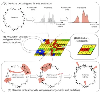
Aevol (www.aevol.fr and references therein) is an in sil-icoexperimental evolution platform developed by the Bea-gle team. Figure 1 presents an overview of the model. Since Aevol has been extensively described in previous publica-tions, here we will only describe its basic organization and focus on the structure of the information coding as it is the target of in our experiments.

Overview The rationale of Aevol is that the structure of the fitness landscape is likely to be strongly determined by the structure of the biological information coding. Hence, Aevol mimics precisely the biological genomic structure as well as the process of genotype-to-phenotype mapping. These structures are then embedded in an evolutionary loop that includes classical selection operators and a large vari-ety of mutational operators including base switch, small in-sertions, small deletions and large scale chromosomal re-arrangements (duplications, deletions, inversions, transloca-tions). All mutation operators have their own rate expressed in mutations.base-pair−1.generation−1(mut.bp−1.gen−1).

Figure 1: The Aevol model. (A) Overview of the genotype-to-phenotype map. (B) Population on a grid and evolution-ary loop. (C) Local selection process with a Moore neigh-borhood. (D) Variation operators include chromosomal re-arrangements and local mutations.

Information coding in Aevol Each individual owns a genome containing its heritable information. The genome is a binary double-strand sequence. It is decoded in two steps: Transcription and Translation. Transcription uses consen-sus promoter signals as starting sequences and hairpin-like structures as terminators. Translation uses consen-sus Ribosome-Binding-Sites (RBS) and an artificial genetic code based on triplet codons (including STARTand STOP

codons). The sequence of codons then constitutes the pri-mary structure of a protein. Importantly, this decoding pro-cess introduces degrees of freedom between the genome and the proteome: complex genomes can encode for simple pro-teomes (e.g. if all genes have the same sequence). On the opposite, complex proteomes can be encoded on small se-quences if genes share sese-quences through e.g. polycistronic mRNA or overlapping genes. These degrees of freedom are similar to the ones real organisms own.

Given the primary structure of a protein, Aevol computes its functional contribution. Although mimicking biological processes at the sequence level is feasible, it is — at least to date — impossible to compute the function of a protein from its primary structure in a realistic way. That is why Aevol uses an abstract mathematical formalism to describe the functional levels (i.e. protein functional contribution and phenotype). In Aevol all functions are expressed in a one-dimensional continuous “functional space” (more precisely on the [0, 1] interval) by an activation value in the [−1, 1] in-terval (upper and lower bounds corresponding to a fully

ac-tivation and to a fully inhibition respectively). In this space, proteins are described as isosceles-triangle-shaped kernel functions. These triangles can themselves be described by three parameters (their mean m, height h and half-width w) which are computed from three interlaced variable-length binary codes in the primary structure of the protein (hence the longer the gene the more precise the m, w and h values). Once all the kernels have been computed from the protein set (Figure 1.A, center), they are summed to compute the phe-notype (Figure 1.A, right). As for the genome-to-proteome step, this procedure introduces degrees of freedom between the proteome and the phenotype. Indeed, the combination of different proteins can result in a simple functional shape e.g. if the proteins share the same m and w values (see Complex-ity measuressection below).

Finally, in Aevol, the fitness is computed as the exponen-tial of the difference between the phenotypic function and a target function indirectly representing the abiotic condi-tions the organisms evolve in (in light red on Figure 1.A, right). Classically in Aevol the target function is defined by a sum of Gaussians, hence requiring a virtually infinite number of triangular kernels to be perfectly fitted. In the experiment described here, we used a modified version of Aevol in which the target function is described by triangles, hence being perfectly fittable by the phenotype (see below).

Experimental design

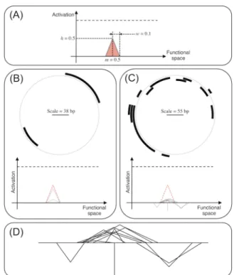
In order to test whether evolution has a spontaneous ten-dency to increase complexity or whether the complexity in-crease is due to the environmental pressure, we let evolve populations of 1,024 individuals in Aevol in a null model where the environment is so simple that it does not require a complex proteome nor a complex genome. To this aim, we designed an environmental target which shape is an isosce-les triangle (Fig. 2.A – to be compared to the classical en-vironment used in Aevol experiments, Figure 1.A, light red filled curve). Hence, the target can be fitted by a single pro-tein and thus a single gene. More precisely, the target is an isosceles triangle with mean m = 0.5, height h = 0.5 and half-width w = 0.1. Note that although this target can be fitted with a single gene, it is still hard to fit since it requires that the corresponding gene be long to get enough precision (see previous section).

All simulations are initialized with a random 5,000 bp genome containing one functional gene. We tested three mutation rates1_{: µ = 10}−4_{, µ = 10}−5 _and

µ = 10−6 mut.bp−1.gen−1. Each population evolved for 270,000 (270k) generations. We then reconstructed the lin-eage of the best final individual and the statistics of the fit-ness, genome size, number of genes and structure of the pro-tein network along the line of descent from generation 0 to

1

We also tested µ = 10−7but evolution was too slow for the data to be usable on 270k generations only.

Figure 2: (A) Phenotypic target used during the experiment. (B, C) Genome (top) and proteome (bottom) of a simple (B) and a complex (C) individual (both evolved exactly in the same conditions; µ = 10−5 mut.bp−1.gen−1). The red dashed line indicates the target function. (D) Zoom on the proteome of the complex individual.

generation 250k (the last 20k generations being canceled be-cause the notion of a fixed lineage vanishes when getting close to the final generation). We then repeated the exper-iment 100 times for each mutation rate for a total of 300 simulated evolutions.

Complexity measures

Generally speaking, there is no consensus on complexity measures. Moreover, since Aevol is a multiscale model, one has to choose different measures for the different lev-els (typically here the sequence level — the genome — and the functional level — the proteome). We thus adopted two strategies. First, we adapted principles from Adami et al. (2000) to Aevol in order to get quantitative measures at the genome and proteome levels by estimating the quantity of information stored in both structures. Second, we designed a qualitative classification of “simple” (S) vs. “complex” (C) organisms based upon the structure of the model.

Quantitative measure at the sequence level Aevol pro-vides numerous statistics on the lineage of a given organ-ism. In particular, it provides statistics about the number of “essential” base pairs (i.e. base pairs which, if mutated, change the phenotype of the organism). Hence, this measure can be directly used to estimate the quantity of information

stored on the genome CG. Note that it may be very

differ-ent from the genome size since the genome can accumulate non-coding sequences. It can also be shorter than the sum of gene lengths since genes can share sequences through gene overlapping.

Quantitative measure at the functional level While measuring complexity on the genome is relatively straight-forward, measuring complexity on the proteome is a more difficult. Indeed, in a first approximation, one could consider that the proteome complexity is given by the number of non-degenerated proteins2_{. However, since different proteins can}

perform similar functions, this would overestimate the quan-tity of information contained in the proteome. Hence, we considered proteome information in a more precise way by estimating the number of different parameters in the pro-teome. The functional complexity measure CP is then the

sum of the number of different m, different w and different h values (all with a small tolerance ε = 0.001 to account for rounding errors) used to encode the protein set.

Qualitative classification To study the long-term fate of simple vs. complex organisms, we defined a qualitative clas-sification procedure. Since the environmental target con-strains the functional (i.e. phenotypic) level we chose to classify organisms according to their functional structure, hence focusing on the proteome level. A simple solution would have been to define a threshold on the quantitative measure but this threshold would be arbitrary. To avoid this, we used knowledge from the model structure to define the two classes. In Aevol, if all the non-degenerated proteins of an organism have the same mean m and the same half-width w, then their functions linearly sum-up to produce a trian-gular phenotype with the same characteristics. We used this property to propose the following classes:

Simple organisms (S – Simples) are organisms for which all the non-degenerated proteins have the same function (i.e., the same m and w values, both with an ε = 0.001 tolerance), possibly with different activity levels (h). Figure 2.B shows an example of a simple individual. Note that all organisms owning a single protein are necessarily simple but that Sim-plesmay contain many genes and many proteins (possibly differing in their h values).

Complex organisms (C – Complexes) are organisms own-ing at least two non-degenerated proteins for which either the triangle mean m or the triangle half-width w values are different (with the same tolerance ε). Figures 2.B and 2.C/D show examples of S and C individuals respectively.

Results

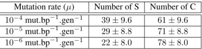
Among the 300 simulations we analyzed, 210 were classi-fied as C (see Methods) at generation 250k. Table 1 shows

2

Degenerated proteins encode for triangles which area is equal to zero (i.e. h = 0 and/or w = 0). These proteins hence don’t contribute to the organism function nor to the phenotype.

the repartition of S and C organisms for the 3 mutation rates. Mutation rate (µ) Number of S Number of C 10−4mut.bp−1.gen−1 39 ± 9.6 61 ± 9.6 10−5mut.bp−1.gen−1 29 ± 8.8 71 ± 8.8 10−6mut.bp−1.gen−1 22 ± 8.0 78 ± 8.0 Table 1: Number of S and C lineages at generation 250k for the three tested mutation rates. 95% Confidence Intervals (CI95%) estimated from the number of samples in both classes:

CI95%= 1.96

p

NSNC/(NS+ NC− 1).

We first verified that the C organisms (resp. S) correspond to those accumulating information (resp. not). Figures 3 and 4 respectively show the amount of information of the proteomes (CP) and the genomes (CG) for S and C organisms

and for all the mutation rates3_.

Figure 3: Distribution of functional complexity CP for the

Complexes (top) and Simples (bottom). Colors indicate the mutation rates. Blue: 10−4 mut.bp−1.gen−1; Red: 10−5mut.bp−1.gen−1; Green: 10−6mut.bp−1.gen−1

Figure 3 clearly shows that Simples tend to accumulate less information in their proteome. The amount of infor-mation in the genome also tends to be smaller for Sim-ples although the trend is less clear (Figure 4). This dif-ference is not surprising given that our qualitative classifi-cation is based on the proteome structure and that Aevol al-lows degrees of freedom between the information coding in the genome and the information coding in the proteins (see Methods). Both figures also show a strong effect of mutation rates: the higher the mutational pressure, the lower CGand

CP. This is not a surprise either, since this effect has already

been described in the literature (Knibbe et al., 2007; Fischer et al., 2014) albeit on the genome size. Contrary to the trend on the amount of information, this effect is more pronounced on the genome, probably because mutational effects directly affect the genome but only indirectly the proteome.

3

Note that CGand CP cannot be quantitatively compared since

they account for information content in a binary sequence and in a set of real values respectively.

Figure 4: Distribution of genomic complexity CG for the

Complexes(top) and Simples (bottom). Same color code as in Figure 3.

Simple organisms are fitter than complex ones

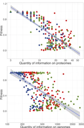
Having observed organisms evolving either simple or com-plex functional structure in the same simple environment, the decisive question is whether or not complexity is driven by selection. Figure 5 shows the fitness of the lineage at generation 250k against CG and CP. It clearly shows that

simpler organisms have a higher fitness than more complex ones. This is confirmed by the fitness distribution among the two qualitative classes (Figure 6): Figure 6 shows that many Simples reach a fitness that approaches 1 (mean fit-ness of Simples: 0.97 ± 0.02), the best possible fitfit-ness in Aevol, while Complexes hardly evolve fitnesses higher than 0.5 (mean fitness of Complexes: 0.38 ± 0.04)

This result demonstrates that in our simulations, the switch between functional simplicity and functional com-plexity is not driven by selection. On the opposite, here, complex functional structures evolve in spite of selection.

Complex organisms evolve greater complexity

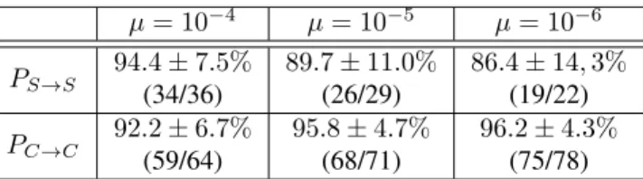
So far we have analyzed only one time point: generation 250k. To address the dynamics of the evolution of com-plexity, we analyzed the fate of S and C organisms between generations 10k and 250k. Table 2 shows that the class (S or C) an organism belongs to at generation 10k is in most cases permanent, suggesting it is part of the organism’s identity.

Table 3 presents the evolution of CG, CP and the fitness

of organisms that retained their S/C identity between gen-erations 10k and gengen-erations 250k. Even though the S→S organisms had their CG decrease, we see that their CP

re-mains constant and their fitness increases only slightly on average. This is because their CP is already very close to

the lower bound at generation 10k, and their fitness already close to the optimum, leaving only so much space for im-provement. On the other hand, the C→C organisms had both their CG and CP but also their fitness increase (Figure 7).

This demonstrates the existence of some kind of

complex-Figure 5: Fitness of the lineage at generation 250k as a func-tion of (top) funcfunc-tional complexity ∼ log(Cp) and (bottom)

genomic complexity ∼ log(CG). Triangles and circles

in-dicate lineages classified as S or C respectively; Same color code as in Figure 3. Linear regressions, top: F itness ∼ log(CP): r-square 0.70 and p-value < 10−15; bottom:

F itness ∼ log(Cg): r-square 0.39 and p-value < 10−15.

Figure 6: Distribution of fitness values at generation 250k for Complexes (top) and Simples (bottom). .

ity ratchet that is stronger than selection (Simples are still far fitter than Complexes) while being created by selection itself (selection tends to make complex organisms become even more complex).

µ = 10−4 µ = 10−5 µ = 10−6 PS→S 94.4 ± 7.5% (34/36) 89.7 ± 11.0% (26/29) 86.4 ± 14, 3% (19/22) PC→C 92.2 ± 6.7% (59/64) 95.8 ± 4.7% (68/71) 96.2 ± 4.3% (75/78) Table 2: Fraction of organisms that conserved their S/C identity between generations 10k and 250k. Values in paren-theses give the number of individuals with identity S (resp. C) at generations 250k and 10k. CI95%computed from the

fractions PI→I and PI→I at generation 250k and NI10k,

the number of individuals of identity I at generation 10k: CI95%= 1.96pPI→IP_I→I/(NI10k− 1).

∆CG ∆CP ∆Fitness

S→S −36.2 ± 14.3 −0.05 ± 0.12 +0.06 ± 0.02 C→C +33.3 ± 23.1 +3.97 ± 0.65 +0.16 ± 0.14 Table 3: Mean CG, CP and Fitness variation between

gen-erations 10k and 250k for organisms that conserved their identity. CI95%computed from the standard deviation and

the number of individuals: CI95%= 1.96pσ2/NI10k.

Figure 7: Evolution of CPin a Complex individual from

gen-eration 0 to gengen-eration 270k.

Effect of robustness constraints on complexity

It is well known that under elevated mutational stress, ro-bust lineages can be selected against fitter ones (Wilke et al., 2001) and that genome compactness is a direct driver of mutational robustness (Knibbe et al., 2007). Hence, if fit-ness cannot drive evolution toward complexity reduction, as shown previously, we hypothesized that robustness could, by imposing a strong complexity limit on the genome.

To test this hypothesis, we submitted the 300 final pop-ulations to a harsh mutation rate during 100k generations. Specifically, each population was further evolved with mu-tation rates 10, 100 and 1,000 times greater than the initial rate (without exceeding the extreme rate of µnew = 10−3)

Table 4 shows the percentage of former complex organisms

having switched to simple (C→S) for the different levels of mutation rate increase.

µ = 10−4 µ = 10−5 µ = 10−6 µnew= 10−3 60 ± 12% (37/61) 86 ± 8% (61/71) 91 ± 6% (71/78) µnew= 10−4 / 8 ± 6% (6/71) 13 ± 8% (13/78) µnew= 10−5 / / 4 ± 4% (3/78) Table 4: Fraction of C→S transitions for all initial (columns) and final (lines) mutation rates. Values in parenthesis give the number of transitions and number of C at generation 250k. CI95%= 1.96pPC→CPC→S/(NC250k− 1).

Among the 600 experiments, 437 started with C organ-isms. 191 (43.7 ± 6.1%) of those switched from C to S (Ta-ble 4). Strikingly, while these C→S organisms experienced a harsh robustness constraint, their fitness strongly increase (mean variation: +0.72 ± 0.04 during the 100k generations of the experiment). In contrast, the 261 C→C organisms experienced a fitness variation of +0.16 ± 0.2. Note that although they retained their C identity, these organisms ex-perienced a strong complexity decrease in reaction to the ro-bustness pressure (CGand CPmean variation: −135.1±21.8

and −2.04 ± 0.78 respectively).

Compared to the proportion of C→S switches in the main experiment, the C→S proportion in this robustness experi-ments is huge, and even more so when focusing on the ex-treme rate µnew = 10−3. Note that the robustness pressure

needs to be very harsh to observe this effect (Table 4). This is probably due to selection for robustness already acting dur-ing the first part of the experiment: at generation 250k the C organisms were probably already robust enough to cope with a reasonable increase in the mutational pressure.

Discussion

By evolving in a very simple environment populations of digital organisms whose complexity can evolve at the ge-nomic and functional levels independently, we were able to acquire important insights into the evolution of complexity. First, the continuous increase in complexity in such a non-demanding environment is a strong argument in favor of a “complexity ratchet”, i.e. an irreversible mechanism that can add components (or information) to the evolving system but that cannot get rid of existing ones, even though this could be more favorable (Cairns-Smith, 1995). Indeed, one of the most astonishing observations is that the complexity ratchet clicks and goes on clicking despite the selective advantage of simple solutions over complex ones. Second, by submit-ting the same organisms to a harsh robustness constraint, we have shown that, contrary to selection for fitness, selection for robustness, when severe, can overcome the ratchet and push complex organisms back toward simplicity.

In our experiments, simple organisms are fitter than com-plex ones. Previous results with Aevol, showed that se-lection for robustness favors streamlined genomes (Knibbe et al., 2007); and that the joint effect of duplications and deletions biases mutations toward reduction (Fischer et al., 2014). Then, if selection, robustness and mutational biases all push in the same direction — simplicity — what is the force that counterbalances them all hence leading to com-plexity increases? To answer this question, we first have to look back at Table 3. It shows that even though Complexes stay far worse than Simples, Complexes still substantially gain fitness between generations 10k and 250k: although complexity increases in spite of selection, its increase is nev-ertheless driven by selection! This immediately points to-ward a negative epistatis phenomenon: mutations that would have been beneficial in a given S individual are deleterious in the genetic context of C individuals (and reciprocally). Indeed, selection only acts on the basis of the local topology of the fitness landscape, which depends on the genetic back-ground of the individuals. In a C genetic context, negative epistasis forbids the acquisition of some genes that could be highly favorable in an S context. Since gene deletion is obvi-ously deleterious, the only available evolutionary path for al-ready complex organisms is a headlong rush toward increas-ing complexity by acquirincreas-ing new genes. Hence the ratchet clicks, further widening the fitness valley that separates the current genome from a simple one, soon making it so wide it is very unlikely to be crossed. Indeed, it has already been shown that in natural populations, epistasis correlates with complexity (Sanju´an and Elena, 2006).

The geometric properties of Aevol functional structure provide a good illustration of the ratchet mechanism. In our experiments, the phenotypic target can only be fitted by a single triangular kernel/protein. However, as soon as the proteome contains a protein with m 6= 0.5 or w 6= 0.1, this is no longer possible because the function that remains to be fitted (i.e. the target minus the protein kernels) becomes multilinear... and the ratchet starts clicking. In other words, each protein added to the proteome increases the complexity of the function that remains to be fitted, forbidding its fitting by a single triangle and triggering further gene recruitment.

Now, if selection cannot overcome the ratchet, how come an increase in mutational pressure can? It is known that se-vere robustness constraints can overcome selection by im-posing an upper limit to the amount of information an or-ganism can transmit to its offspring at the genetic (Eigen and Schuster, 1977) and at the genomic (Knibbe et al., 2007; Fischer et al., 2014) levels. In our experiments, raising the mutation rate strongly decreases the storage capacity of the genome, hence forcing gene elimination despite the fitness loss. This can lower epistatic constraints enough to allow the transition from complexity to simplicity.

Table 1 shows that the ratchet does not systematically start clicking: in nearly one third of our simulations, evolution

leads to simple solutions. Moreover, we saw that the path toward simplicity or complexity is taken very early in the simulations (often before generation 1,000, data not shown) which indirectly confirms that the ratchet is engaged when the organisms recruits its first genes. But how is this initial direction determined? Starting with a single gene, the or-ganisms can evolve in two ways: (1) optimizing this gene by mutation, (2) recruiting new genes through a duplication-divergence mechanism. Depending on this highly contin-gent alternative, evolution is more or less likely to lead to either S or C identity. However, selection can also play its role: since the former path gives higher fitnesses, clonal in-terference between both paths is likely to favor simplicity. Hence, if our explanation is correct, the fraction of Simples should increase in very large populations (clonal interfer-ence being more frequent in large populations).

Finally, if contingency explains the initiation of the ratchet and epistasis explains its mechanisms, what about its long term behavior? Will the ratchet click forever, thus reaching very high complexities? In our simulations the fi-nal complexity seems to be bound despite a great room for improvement in most of the C organisms (Fig. 5). Three effects can bound complexity: (1) As complexity grows, the advantage provided by new genes may become too small for selection to allow their fixation. Indeed, Lynch and Conery (2003) proposed that genome complexity is mainly driven by population genetics effects. However this is unlikely to explain the apparent bound we observe since Complexes can still improve greatly (Fig. 6). (2) Proteome complexity needs to be encoded in the genome but there is an upper bound to the amount of information a genome (hence a pro-teome) can carry with given mutation (Eigen and Schuster, 1977) and rearrangement (Fischer et al., 2014) rates. (3) The waiting time to the next innovation grows as the organism becomes more complex. Indeed, it is well known that evo-lution suffers from a “cost of complexity” that slows down adaptation as the number of selected traits increases (Orr, 2000). In our simulation, Simples fit the target globally — as a single trait — while Complexes virtually split the target in parts which they fit more or less independently. Hence Complexesare likely to suffer from the cost of complexity: complexity increase can slow down in such a way that it would require virtually-infinite waiting time to approach the two above-mentioned bounds.

When experimenting with models, a tricky question is al-ways to tell evolutionary trends apart from model artifacts. Here, we used Aevol, a model that has already proven its consistency, but that nevertheless has its limits. Among them, three at least are likely to interfere with our results. First, as in all ALife models, we deal with very small popu-lations compared to natural popupopu-lations. Larger population size may change the initial direction toward S or C or the upper complexity bounds but since selection cannot invert the ratchet we hypothesize that our conclusions qualitatively

hold whatever the size of the population. Second, the prop-erties of our artificial chemistry may differ from real bio-chemistry. In particular, dosage effects are stronger in Aevol than in Nature. However, this property is likely to limit the complexity increase since gene duplications are more delete-rious in the model than in Nature. Then, this should not alter our main conclusions. Last but not least, although Aevol is a multi-scale model, it lacks some scales that are likely to play a crucial role in the evolution of complexity. In par-ticular it lacks a complex ecosystem and a gene network. Hence, we cannot observe here the effect of niche construc-tion that are often proposed as a major player in the evo-lution of complexity. On the gene network side, our results match very well those we got when we used the RAEvol ver-sion of the model to evolve genetic networks in constant vs. variable environments (Beslon et al., 2010; Vad´ee-Le-Brun et al., 2016). Indeed, in these experiments the complexity of the network appeared to be driven by the mutation rate and highly complex networks evolved even in constant environ-ments. This opens the interesting perspective of replicating the present experiments in RAevol.

Our work opens many other perspectives. Specifically, we would like to analyze the evolutionary dynamic of our pop-ulations at a finer grain. In particular, analyzing the effect of every single mutation on complexity, fitness, evolvability and robustness depending on the mutation type (point mu-tations vs. rearrangements) would allow for a better char-acterization of the epistatic interactions in the model. Fi-nally, the most engaging perspective would be to generalize the mechanism observed here to other kinds of systems. In-deed, an open question is whether this complexity ratchet could contribute to Open-Ended Evolution (Banzhaf et al., 2016), hence opening the door for non-selectively-driven Open-Endedness. A difficult question here is whether epis-tasis has an equivalent in other Open-Ended systems such as economy or innovation.

In conclusion, we would like to stress that our results, gathered on a null model, do not imply that there is no such thing as selection for complexity. But importantly, they show that selection for complexity is not mandatory for complexity to evolve. Hence, complex biological structures could flourish in conditions where complexity is not needed. Reciprocally, the global function of these complex structures could very well be simple. We think this result is greatly sig-nificant for both evolutionary biology and systems biology.

References

Adami, C. (2002). What is complexity? BioEssays, 24(12):1085– 1094.

Adami, C., Ofria, C., and Collier, T. C. (2000). Evolution of bio-logical complexity. PNAS, 97(9):4463–4468.

Banzhaf, W., Baumgaertner, B., Beslon, G., Doursat, R., Fos-ter, J. A., McMullin, B., De Melo, V. V., Miconi, T., Spec-tor, L., Stepney, S., et al. (2016). Defining and

simulat-ing open-ended novelty: requirements, guidelines, and chal-lenges. Theory in Biosciences, 135(3):131–161.

Batut, B., Knibbe, C., Marais, G., and Daubin, V. (2014). Reduc-tive genome evolution at both ends of the bacterial population size spectrum. Nature Reviews Microbiology, 12(12):841. Batut, B., Parsons, D. P., Fischer, S., Beslon, G., and Knibbe, C.

(2013). In silico experimental evolution: a tool to test evolu-tionary scenarios. In BMC bioinfo, volume 14, page S11. Beslon, G., Parsons, D. P., Sanchez-Dehesa, Y., Pena, J.-M., and

Knibbe, C. (2010). Scaling laws in bacterial genomes: A side-effect of selection of mutational robustness? Biosystems, 102(1):32–40.

Cairns-Smith, A. (1995). The complexity ratchet. In Progress in the Search for Extraterrestrial Life., volume 74, page 31. Eigen, M. and Schuster, P. (1977). A principle of natural

self-organization. Naturwissenschaften, 64(11):541–565. Fischer, S., Bernard, S., Beslon, G., and Knibbe, C. (2014).

A model for genome size evolution. Bull. Math. Biol., 76(9):2249–2291.

Gould, S. J. (1996). Full House: The Spread of Joy from Plato to Darwin. Harmony Books.

Hahn, M. W., Wray, G. A., et al. (2002). The g-value paradox. Evolution and Development, 4(2):73–75.

Knibbe, C., Coulon, A., Mazet, O., Fayard, J.-M., and Beslon, G. (2007). A long-term evolutionary pressure on the amount of noncoding dna. Mol. Biol. Evol., 24(10):2344–2353. Lynch, M. and Conery, J. S. (2003). The origins of genome

com-plexity. Science, 302(5649):1401–1404.

McShea, D. W. (1996). Metazoan complexity and evolution: Is there a trend? Evolution, 50(2):477–492.

Miconi, T. (2008). Evolution and complexity: The double-edged sword. Artificial life, 14(3):325–344.

Orr, A. H. (2000). Adaptation and the cost of complexity. Evolu-tion, 54(1):13–20.

Sanju´an, R. and Elena, S. F. (2006). Epistasis correlates to genomic complexity. PNAS, 103(39):14402–14405.

Soyer, O. S. and Bonhoeffer, S. (2006). Evolution of complexity in signaling pathways. PNAS, 103(44):16337–16342.

Thomas, C. A. J. (1971). The genetic organization of chromo-somes. Annual review of genetics, 5(1):237–256.

Vad´ee-Le-Brun, Y., Rouzaud-Cornabas, J., and Beslon, G. (2016). In silico experimental evolution suggests a complex inter-twining of selection, robustness and drift in the evolution of genetic networks complexity. In ALife XIV, pages 180–188. Wilke, C. O., Wang, J. L., Ofria, C., Lenski, R. E., and Adami, C.

(2001). Evolution of digital organisms at high mutation rates leads to survival of the flattest. Nature, 412(6844):331. Yaeger, L., Griffith, V., and Sporns, O. (2008). Passive and driven

trends in the evolution of complexity. In ALife XI, pages 725– 732.