HAL Id: hal-01589251
https://hal.archives-ouvertes.fr/hal-01589251
Submitted on 18 Sep 2017
HAL is a multi-disciplinary open access
archive for the deposit and dissemination of
sci-entific research documents, whether they are
pub-lished or not. The documents may come from
teaching and research institutions in France or
abroad, or from public or private research centers.
L’archive ouverte pluridisciplinaire HAL, est
destinée au dépôt et à la diffusion de documents
scientifiques de niveau recherche, publiés ou non,
émanant des établissements d’enseignement et de
recherche français ou étrangers, des laboratoires
publics ou privés.
Temporal Reprogramming of Boolean Networks
Hugues Mandon, Stefan Haar, Loïc Paulevé
To cite this version:
Hugues Mandon, Stefan Haar, Loïc Paulevé. Temporal Reprogramming of Boolean Networks. CMSB
2017 - 15th conference on Computational Methods for Systems Biology, Sep 2017, Darmstadt,
Ger-many. pp.179 - 195, �10.1007/978-3-319-67471-1_11�. �hal-01589251�
Temporal Reprogramming of Boolean Networks
?Hugues Mandon1,2, Stefan Haar1, Lo¨ıc Paulev´e2
1 LSV, ENS Cachan, INRIA, CNRS, Universit´e Paris-Saclay, France 2
LRI UMR 8623, Univ. Paris-Sud – CNRS, Universit´e Paris-Saclay, France
Abstract. Cellular reprogramming, a technique that opens huge op-portunities in modern and regenerative medicine, heavily relies on iden-tifying key genes to perturb. Most of computational methods focus on finding mutations to apply to the initial state in order to control which attractor the cell will reach. However, it has been shown, and is proved in this article, that waiting between the perturbations and using the tran-sient dynamics of the system allow new reprogramming strategies. To identify these temporal perturbations, we consider a qualitative model of regulatory networks, and rely on Petri nets to model their dynamics and the putative perturbations. Our method establishes a complete charac-terization of temporal perturbations, whether permanent (mutations) or only temporary, to achieve the existential or inevitable reachability of an arbitrary state of the system. We apply a prototype implementation on small models from the literature and show that we are able to derive temporal perturbations to achieve trans-differentiation.
1
Introduction
Regenerative medicine is gaining traction with the discovery of cell reprogram-ming, a way to change a cell phenotype to another, allowing tissue or neuron regeneration techniques. After proof that cell fate decisions could be reversed [17], scientists need efficient and trustworthy methods to achieve it. Instead of producing induced pluripotent stem cells and force the cell to follow a distinct differentiation path, new methods focus on trans-differentiating the cell, without necessarily going (back) through a multipotent state [9,8].
This paper addresses the formal prediction of perturbations for cell repro-gramming from computational models of gene regulation. We consider qualita-tive models where the genes and/or the proteins, notably transcription factors, are nodes with an assigned value giving the level of activity, e.g., 0 for inactive and 1 for active, in a Boolean abstraction. The value of each node can then evolve in time, depending on the value of its regulators.
The attractors, or long term dynamics, of qualitative models typically corre-spond to differentiated and stable states of the cell [13,18]. In such a setting, cell
?This research was supported by Labex DigiCosme (project
ANR-11-LABEX-0045-DIGICOSME) operated by ANR as part of the program “Investissement d’Avenir” Idex Paris-Saclay (ANR-11-IDEX-0003-02); by ANR-FNR project “AlgoReCell” (ANR-16-CE12-0034); and by CNRS PEPS INS2I 2017 “FoRCe”.
reprogramming can be interpreted as triggering a change of attractor: starting within an initial attractor, perform perturbations which would de-stabilize the network and lead the cell to a different attractor.
Current experimental settings and computational models mainly consider cell reprogramming by applying the set of perturbations simultaneously in the initial state. However, as suggested in [14] and as we will demonstrate formally in this paper, considering temporal reprogramming, i.e., the application of per-turbations in particular moments in time, and in a particular ordering, brings new reprogramming strategies, potentially requiring fewer interventions. Contribution This paper establishes the formal characterization of all possible reprogramming paths between two states of asynchronous Boolean networks by the means of a bounded number of either permanent (mutations) or temporary perturbations. Solutions account both for perturbations applied only in the ini-tial state, and perturbations applied in a specific ordering and in specific states. Moreover, the solutions can guarantee that the target state may be reached, or will be reached inevitably.
Our method relies on a Petri net modelling jointly the asynchronous dynamics of the Boolean network and the candidate perturbations. The reprogramming solutions are identified from the state transition graph of the resulting model. We apply our approach on biological networks from the literature, and show that the temporal application of perturbations brings new reprogramming solutions. Related work The computational prediction for reprogramming of Boolean net-works has been addressed mainly by considering mutations to be applied in the initial state only, letting then the system stabilize itself in the targeted attrac-tor [6,19,15,1,7,16]. Our method includes temporal perturbations, which none of these methods do: perturbations which takes into account the latent dynamics of the system for the reprogramming, allowing more solutions to be found, and possibly some needing fewer nodes to be perturbed.
Other approaches consider stochastic frameworks for exploring by simulation potential reprogramming event in Boolean networks, such as [10] for stochastic transitions between cell cycles. Statistical methods are also used to extract com-binations of transcription factors that are key for cellular differentiation from gene expression data [14,3]. In [14], starting from expression data, they derive a continuous dynamical model from which control strategies for reprogramming can be computed. They show that time-dependent perturbations can provide potential reprogramming strategies.
Most of mentioned methods provide incomplete or non-guaranteed results. Our aim is to provide a formal framework for the complete and exact character-isation of the initial state and temporal reprogramming of Boolean networks. Outline Sect. 2 details an example of Boolean network which motivates temporal reprogramming. Sect. 3 introduces our model of temporal reprogramming, Sect. 4 establishes the identification of temporal reprogramming strategies, and Sect. 5 applies it to biological networks from the literature. Sect. 6 concludes the paper.
Notations: The set {1, ..., n} is noted [n]; Given x ∈ {0, 1}n and i ∈ [n], ¯x{i} ∈ {0, 1}n is such that for all j ∈ [n], ¯x{i}
j ∆ = ¬xj if j = i and ¯x {i} j ∆ = xj if j 6= i.
2
Background and Motivating Example
This section illustrates the benefit of temporal reprogramming on a small Boolean network in order to trigger a change of attractor. We consider both perturba-tions to be applied solely in the initial state, and perturbaperturba-tions to be applied in a specific sequence in specific states. We show that, in the first setting, 3 perturbations are always required for the reprogramming, whereas the temporal approach necessitates only 2.
2.1 Boolean networks
A Boolean Network is a tuple of Boolean functions giving the future value of each node with respect to the global state of the network.
Definition 1 (Boolean Network (BN)). A Boolean Network of dimension n is a function f such that:
f : {0, 1}n→ {0, 1}n
x = (x1, ..., xn) 7→ f (x) = (f1(x), ..., fn(x))
The dynamics of a Boolean network f are modelled by transitions between its states x ∈ {0, 1}n. In the scope of this paper, we consider the asynchronous semantics of Boolean networks: a transition updates the value of only one node i ∈ [n]. Thus, from a state x ∈ {0, 1}n, there is one transitions for each vertex i such that fi(x) 6= xi. The transition graph (Def. 2) is a digraph where vertices are all the possible states {0, 1}n, and edges correspond to asynchronous transitions. The transition graph of a Boolean network f can be noted as STG(f )
Definition 2 (Transition graph). The transition graph (also known as state graph) is the graph having {0, 1}n as vertex set and the edges set {x → ¯x{i} | x ∈ {0, 1}n, i ∈ [n], fi(x) = ¬xi}. A path from x to y is noted x →∗y.
The terminal strongly connected components of the transition graph can be seen as the long-term dynamics or “fates” of the system, that we refer to as attractors. An attractor may model sustained oscillations (cyclic attractor ) or a unique state, referred to as a fixpoint, f (x) = x.
2.2 Cell reprogramming: the advantage of temporal perturbations Let us consider the following Boolean Network:
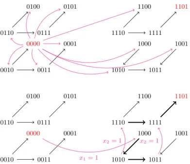
Fig. 1 gives the transition graph of this Boolean Network, and the different perturbation techniques. To understand the benefit of temporal perturbations, let us consider the perturbations to apply in the fixpoint 0000 in order to reach the fixpoint 1101.
Because 0000 is a fixpoint, there exists no sequence of transitions from 0000 to 1101. It can also be seen that if one or two vertices are perturbed at the same time, by affecting them new values, 1101 is not reachable, as shown in Fig. 1(top). However, if two vertices are perturbed, but the system is allowed to follow its own dynamics between the changes, 1101 can be reached, as shown in Fig. 1(bottom), by using the path 0000 x1=1
−−−→ 1000 → 1010 → 1011 x2=1
−−−→ 1111 → 1101, i.e. we first force the activation of the first node, then wait until the system reaches (by itself) the state 1011 before activating node 2. From the perturbed state, the system is guaranteed to end up in the wanted fixpoint, 1101.
Inevitable and existential reprogramming Thus, this example shows that some attractors may be reached by changing the values of vertices in a particuliar order and using the transient dynamics. We remark that there exists another reprogramming path, where node 2 is perturbed when the system reach 1010. Note that, in this case, after the second perturbation, the system can reach 1101, but it is not guaranteed. We say that, in the first reprogramming path, the reprogramming is inevitable, whereas it is only existential in the second case. Permanent and temporary solutions The previous example shows the difference between what we will call temporal and initial reprogramming. How perturba-tions are made has also to be considered. The model can either only be slightly perturbed, by changing the value of a vertex i for a time (setting i to 0 or 1), or the change can be permanent, by changing the function of the vertex (setting fi to 0 or 1). On the example above, making permanent changes would not change the solutions found. However, if the initial state is 1011 and the target state is 1100, then it has different solutions (Fig. 2).
Indeed, if the objective is to go from 1011 to 1100 in the same transition graph using only permanent perturbations, then their order does not matter. Perturbating x2 and x4 from the initial state is enough to make 1100 the only reachable state. On the other hand, if the perturbations are temporary, x2 has to be perturbed first, then when 1101 is reached, x4 can be perturbed. If this order is not followed, 1101 is reachable as well as 1100.
In most case, the perturbations done in permanent reprogramming and the ones done in temporary reprogramming can be on different nodes.
3
Modelling Temporal Reprogramming with Petri Nets
In this section, we introduce a new model for the temporal reprogramming of Boolean Networks (BNs) using Safe (1-bounded) Petri nets [2]. We take ad-vantage of the transition-centred specification of Petri nets and their ability to
0000 0001 0010 0011 0100 0101 0110 0111 1000 1001 1010 1011 1100 1101 1110 1111 0100 0000 0001 0010 0011 0101 0110 0111 1000 1001 1010 1011 1100 1101 1110 1111 x1 = 1 x2= 1 x2= 1
Fig. 1. Transition graph of f and candidate perturbations (magenta) for the repro-gramming from 0000 to 1101: (top) none of candidate perturbations of one or two nodes in the initial state allow to reach 1101; (bottom) sequences of two temporal perturbations allow to reach 1101.
1000 1001 1010 1011 1100 1101 1110 1111 1000 1001 1010 1011 1100 1101 1110 1111 \ x2 = 1, x4= 0 x2= 1 x4 = 0
Fig. 2. Right part of the transition graph of f from initial state 1011 to 1100, with permanent perturbations (left) and temporary ones (right)
define specific coupled transitions (the simultaneous change of value of several components) to model the candidate perturbations.
Definition 3 (Safe Petri Net). A Petri net is a tuple (P, T, A, M0) where P and T are sets of nodes, called places and transitions respectively, and A ⊆ (P × T ) ∪ (T × P ) is a flow relation whose elements are called arcs. A subset M ⊆ P of the places is called a marking, and M0 is a distinguished initial marking.
For any node u ∈ P ∪ T , we call pre-set of u the set •u = {v ∈ P ∪ T | (v, u) ∈ A} and post-set of u the set u•= {v ∈ P ∪ T | (u, v) ∈ A}.
A transition t ∈ T is enabled at a marking M if and only if•t ⊆ M . The application of such a transition leads to the new marking M0= (M \•t) ∪ t•, and is denoted by M −→ Mt 0. A marking M0 is reachable if there exists a sequence of transitions t1, . . . , tk such that M0 t1
−→ . . . tk
−→ M0.
A Petri net is safe if and only if any reachable marking M is such that for any t ∈ T that can fire from M leading to M0, the following property holds: ∀p ∈ M ∩ M0, p ∈•t ∩ t•∨ p /∈•t ∪ t•.
Less formally, a safe Petri Net is a Petri Net where in all reachable markings from the initial marking, all places have at most one token. A subset of places {p1, . . . , pk} ⊆ P is mutually exclusive if every reachable marking M contains at most one these place.
3.1 Encoding asynchronous Boolean networks
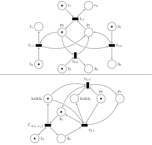
The equivalent representation of the asynchronous semantics of a Boolean net-work of dimension n f = (f1, · · · , fn) in Petri net has been addressed in [4,5]. Essentially, to each node i ∈ [n] of the Boolean network f is associated two places, i0 and i1, acting respectively for the node i being inactive and active. Then, transitions are derived from clauses of the Disjunctive Normal Form (DNF; disjunction of conjunctive clauses) representation of [¬xi∧ fi(x)] for i activation, and from [xi∧ ¬fi(x)] for i inactivation.
Given a logical formula [e], we write DNF[e] for its DNF representation. DNF[e] is thus a set of clauses, where clauses are sets of literals. A literal corre-spond to the state of a node, and is either of the form xi(node i is active), or ¬xi (node i is inactive). Given such a literal l, place(l) associates the corresponding Petri net place: place([xi])= i1∆ and place([¬xi])∆= i0.
The safe Petri net encoding the asynchronous semantics of a Boolean network f is defined as follows.
Definition 4 (PN(f )). Given a Boolean network f of dimension n and an ini-tial state x ∈ {0, 1}n, PN(f ) = (Pf, Tf, Af, M0) is the corresponding Safe Petri Net such that:
– Pf =S
i∈[n]{i0, i1} is the set of places,
• for each clause c ∈ DNF[¬xi∧ fi(x)], there is a transition ti,c∈ Tf with Af such that •ti,c= {place(l) | l ∈ c} and ti,c•= {i1} ∪•ti,c\ {i0}; • for each clause c ∈ DNF[xi∧ ¬fi(x)], there is a transition t¬i,c∈ Tf with
Af such that •t¬i,c= {place(l) | l ∈ c} and t¬i,c•= {i0} ∪•t¬i,c\ {i1}, – M0= {ixi | i ∈ [n]} is the initial marking.
Note that [5] also extends the encoding to multi-valued networks into 1-bounded Petri nets (contrary to the encoding of multi-valued networks of [4] which does not result in a safe Petri net). For the sake of simplicity, we re-strict the presentation to Boolean networks. However, our encoding of temporal perturbations can be easily extended to multi-valued networks.
Example 1. Fig. 3 gives the resulting Petri net encoding of the Boolean function f3(x) = x1∧ ¬x2. In this case, DNF[¬x3∧ (x1∧ ¬x2)] = {{¬x3, x1, ¬x2}} and DNF[x3∧ (¬x1∨ x2)] = {{x3, ¬x1}, {x3, x2}}.
3.2 Encoding temporal perturbations
Perturbations are modelled as additional transitions which modify the state of nodes of the BN f . These perturbations can be performed at any time during the transient dynamics, and independently of the current state of the network.
In the scope of this paper, we consider two kinds of perturbations: tempo-rary perturbations induce a state change of nodes, but these nodes can later be updated according to their Boolean function. Such perturbations can model, for instance, the transient activation of transcription factor through a signalling pathway. Permanent perturbations induce a permanent state change of nodes. These perturbations model mutations (loss or gain of functions).
In both cases, we consider a limited amount of allowed perturbations: only up to k successive perturbations can be performed.
Temporary perturbations In addition to the places for the BN node values, we add k mutually exclusive places c1, . . . , ck and two mutually exclusive places p0 and p1. Essentially, cj is marked if the next perturbation is the j-th; and p0 is marked if the j-th perturbation is yet to be performed, and p1 is marked if the j-th perturbation has been performed.
The transitions are the same as in PN(f ), with additional transitions ti,0and ti,1 for each node i ∈ [n] which set their value to 0 and 1 respectively. To be enabled, these transitions need p0 to be marked, and after the transition, p1 is marked. Finally, a transition tcj re-enabling p0is defined for each cj, j ∈ [k − 1], which moves the marking of cj to cj+1.
Definition 5. Given a Boolean network f of dimension n, the Petri net (P, T, A, M0) modelling its k temporary perturbations is given by
– P = Pf∪ {p0, p1, c1, . . . , ck},
31 11 10 30 20 21 t¬3,{¬x1} t¬3,{x2} t3,{x1,¬x2}
Fig. 3. Safe Petri net encoding of f3(x) = x1∧ ¬x2. Places are drawn as circles and
transitions as rectangles. Marked places have a dot. c1 tc1 c2 p0 p1 t1,1 11 10 t2,0 21 20 t3,0 31 30 31 lock30 lock31 t3,10 p0 p1 t3,1 t0¬3,{¬x1} 30 10
Fig. 4. (top) Excerpt of the encoding of temporary perturbations. (bottom) Excerpt of the encoding of permanent perturbations.
(a) BN transitions Tf ⊆ T , Af ⊆ A; (b) Perturbation transitions for i ∈ [n],
ti,0∈ T with •ti,0= {i1, p0} and ti,0•= {i0, p1} ti,1∈ T with •ti,1= {i0, p0} and ti,1•= {i1, p1}; (c) Perturbation enabling for j ∈ [k − 1],
tcj ∈ T with •tcj = {p1, cj} and tcj•= {p0, cj+1}, – M0= {ixi | i ∈ [n]} ∪ {p0, c1},
where (Pf, Tf, Af, M00) = PN(f ).
Example 2. Fig. 4(top) shows part of the transitions added by the modelling of k = 2 temporary perturbations in the example of Fig. 3. In the given marking, the perturbation are enabled, therefore, any of the 3 shown perturbation tran-sitions can be applied. The application of one such transition disable the other perturbation transitions (as p0is no longer marked). By applying the transition tc1, the perturbations transitions are then re-enabled, allowing a second (and last) one to be applied.
Permanent perturbations (mutations) Contrary to temporary perturba-tions, once a node has been (permanently) perturbed, its state should no longer change. This is modelled by locks: if the i-th lock is active the node i cannot perform any transition. In addition to the places introduced for temporary per-turbations, our encoding add mutually exclusive places locki0, locki1 for each each node i ∈ [n], locki0 being marked if the node i has not been perturbed, locki1 being marked otherwise.
The transitions of the BN are then modified so that a transition changing the state of node i requires the place locki0 to be marked. For each node i, 4 perturbations transitions are defined: two for the value changes (0 to 1 and 1 to 0) also inducing the marking of locki1; and two for the marking of locki1without value change: indeed, a mutation does not necessarily have to change the current value of the node, but it prevents any further evolution of it.
Definition 6. Given a Boolean network f of dimension n, the Petri net (P, T, A, M0) modelling its k permanent perturbations is given by
– P = Pf∪ {p0, p1, c1, . . . , ck} ∪S
i∈[n]{locki0, locki1} – T and A are the smallest sets which satisfy
BN transitions ∀tl,c∈ Tf, with l = i or l = ¬i, i ∈ [n],
t0l,c∈ T with •t0l,c=•tl,c∪ {locki0} and t0l,c•= tl,c•∪ {locki0} Perturbation transitions for i ∈ [n],
ti,0∈ T with •ti,0= {i1, p0, locki0} and ti,0•= {i0, p1, locki1} ti,00 ∈ T with •ti,00 = {i0, p0, locki0} and ti,00•= {i0, p1, locki1}
ti,1∈ T with •ti,1= {i0, p0, locki0} and ti,1•= {i1, p1, locki1} ti,10 ∈ T with •ti,10 = {i1, p0, locki0} and ti,10•= {i1, p1, locki1}
Perturbation enabling for j ∈ [k − 1],
– M0= {ixi | i ∈ [n]} ∪ {p0, c1} where (Pf, Tf, Af, M00) = PN(f ).
Example 3. Fig. 4(bottom) shows part of the transitions added by the modelling of k = 2 permanent perturbations. The transition t3,{¬x1} of Fig. 3 is modified so that it is enabled only if lock30 is marked, i.e., the node 3 has not been perturbed yet. Permanent perturbation transitions t3,1 and t3,10 lock the node 3
to its value 1. Once applied, none of the transitions modifying the value of node 3 can be enabled. Transitions for re-enabling perturbations are identical to the temporary case.
3.3 State Transition Graph
Given a BN f and an initial state x, the above modelling allows to compute all the states reachable by any combination and succession of k perturbations, temporary or permanent.
The next section establishes the complete characterisation of perturbations for the existential and inevitable reprogramming of f from x. It relies on an explicit state transition graph which is composed of two classes of transitions: the transitions induced by BN f , and the transitions induced by the perturbation.
It can be remarked that our encoding uses an additional kind of transition: the transitions for re-enabling the perturbation transitions, when strictly less than k perturbations have been applied (transitions noted tcj, j ∈ [k − 1]). These transitions are artefacts of the modelling, and can be skipped during the state transition graph construction.
Let us define a state transition graph among states S with two classes of transitions E (induced by f ) and M (induced by the perturbations), as the smallest digraph (S, E , M) such that M0 ∈ S, and for each M ∈ S, for each t ∈ T such that•t ⊆ M , let M0= (M \•t) ∪ t•,
– if p1∈ M and ck ∈ M , then ∃j ∈ [k] :/ •tcj ∈ M0; let M00= (M0\•tcj) ∪ tcj•, M00∈ S and (M, M00) ∈ E,
– otherwise, M0 ∈ S, and if t = tl,c, then (M, M0) ∈ E , else (M, M0) ∈ M. Given any marking M ∈ S of the resulting state transition graph, the number of perturbations applied to reach M is given by j + b where cj∈ M and pb∈ M .
4
Complete Identification of Temporal Reprogramming
Strategies
This section explains how, from the transition graph obtained by the model of Sect.3, the complete set of reprogramming solutions leading to a set of final states F ⊆ S can be identified.
The Perturbation Transition Graph (Def. 7) gathers the transitions of the Boolean network from the state x, and the perturbation transitions with a label
specifying the performed perturbation. Each node of the original transition graph have multiple copies, given how many perturbations are used to reach it: thus, a state of the perturbation transition graph is composed of the state of the Boolean network and a perturbation counter. A transition of the Boolean network is necessarily between two states with the same counter; a perturbation transition is necessarily between a state with counter i to a state with counter i + 1. This Perturbation Transition Graph can be directly computed from the Petri net of Sect. 3. Given a subset M of perturbation transitions, a Perturbation Path (Def.8) is a sequence of Boolean networks transitions and transitions in M . Definition 7 (Perturbed Transition Graph). Given a Boolean network f of dimension n and a maximum number of allowed perturbations k, the Perturbed Transition Graph is a tuple (S0, E0, M0) where
– S0= {0, 1}n× {0, .., k} is the set of states;
– E0 ⊆ {(s, i) → (s0, i) | i ∈ [0; k], (s → s0) ∈ Ef}, where STG(f ) = ({0, 1}n, E
f), is the set of normal transitions, which corresponds to a subset of the asynchronous transitions of the Boolean network f ;
– M0⊆ {(s, i) → (s0, i + 1) | i ∈ [0; k − 1], s, s0 ∈ {0, 1}n} × L is a set of per-turbation transitions, where L is the set of labels describing the perper-turbation. Definition 8 (Perturbation path (→∗M)). Given a Perturbation State Graph (S, E , M) and a set of perturbation transitions M ⊆ M, →∗M⊆ S × S is a binary relation such that
(s, i) →∗M (s0, i0) ∆
⇔ (s, i) = (s0, i0) or ∃(s00, i00) ∈ S with
(s, i) → (s00, i00) ∈ E ∪ M and (s00, i00) →∗M (s0, i0)
4.1 Complete identification of reprogramming solutions
In the scope of this paper, we consider two classes of reprogramming solutions: the reprogramming solutions which build a path that reaches one of the final states, referred to as existential reprogramming (Def .9); and the reprogram-ming solutions which ensure that a final state is always reached, referred to as inevitable reprogramming (Def. 10)
Definition 9 (Existential Reprogramming). Given a Perturbation Tran-sition Graph (S, E , M) of a Boolean network f , a state (s0, i0) ∈ S has an existential reprogramming to a set of states F ⊆ S if and only if there exists a set of perturbation transitions M ⊆ M such that there is a path from (s0, i0) to a state w ∈ F using only E and M transitions, i.e., (s0, i0) →∗M w.
Definition 10 (Inevitable Reprogramming). Given a Perturbation Tran-sition Graph (S, E , M) of a Boolean network f , a state (s0, i0) ∈ S has an inevitable reprogramming to a set of states F ⊆ S if and only if there exists a set of perturbation transitions M ⊆ M such that from any state (s, i) ∈ S reachable from (s0, i0) using E and M transitions, there exists a path from (s, i) to a state in F using E and M transitions: ∀(s, i) ∈ S with (s0, i0) →∗M (s, i), ∃w ∈ F such that (s, i) →∗
Given a reprogramming property, the set of nodes that verify it (called “valid nodes” below) can be computed iteratively, by browsing the transition graph in a reverse topological order of the strongly connected components. As a topological order is used, the complexity is linear in the number of states in the Perturbed Transition Graph.
It can be noted that all strongly connected components have the same value of perturbations counter, as there are no edges that decrease the counter. As a consequence, all edges between two strongly connected components are either only normal edges, or only perturbation edges.
In the following part, we only consider the condensed graph G = (S, E , M) of the perturbed transition graph. For a graph G0= (S0, E0, M0), the condensed transition graph G, is defined by:
– A set of strongly connected components of the states. ∀u ∈ S0, ∃s ∈ S, u ∈ s. S is a partition of S0.
– A set of normal edges between the strongly connected components: E = {((s, i) → (s0, i)) | s, s0 ∈ S, ∃s0 ∈ s, s0
0 ∈ s0 such that ((s0, i) → (s00, i)) ∈ E0}
– A set of perturbation edges between the strongly connected components: M = {((s, i)−→ (sl 0, i + 1)) | s, s0 ∈ S, ∃s0 ∈ s, s0 0 ∈ s0 such that ((s0, i) l − → (s00, i + 1)) ∈ M0}
Given the construction of the graph, G is a Perturbed Transition Graph as well.
Existential Reprogramming: In the case of existential reprogramming, a node is valid if it is one of the final nodes or if it has an edge (a normal edge or a perturbation edge) that leads to a valid node.
Definition 11. Given a Perturbation Transition Graph (S, E , M), the set of valid nodes for existential reprogramming VE ⊆ S is defined by:
VE= {(u, i) ∈ S | ∃M ⊆ M, ∃(v, j) ∈ F , (u, i) →∗M (v, j)}
Inevitable reprogramming: In the case of inevitable reprogramming, a valid node is either: a) a final node, b) a node from which all children through nor-mal edges are valid nodes, or c) a node that reaches a valid node through one perturbation edge.
Definition 12. Given a Perturbation Transition Graph (S, E , M), the set of valid nodes for inevitable reprogramming VI ⊆ S is defined by:
VI = {(u, i) ∈ S | ∃M ⊆ M, ∃(v, j) ∈ F , (u, i) →∗M (v, j) and ∀(u 0, i0) ∈ S verifying (u, i) →∗
M (u0, i0), ∃(v0, j0) ∈ F , (u0, i0) →∗M (v0, j0)}
Validity of the initial node: If the initial node is not valid as defined above, then there is no reprogramming solution given the settings. Otherwise, there exist one or more paths that correspond to reprogramming solutions. This will be illustrated on examples from the literature in Sect. 5.
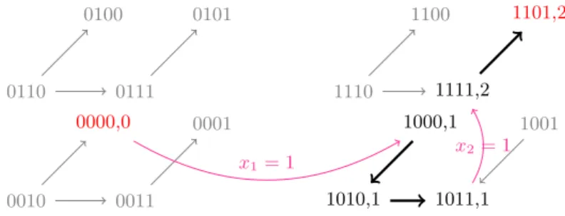
0000,0 0001 1000,1 1010,1 1011,1 1111,2 1101,2 0010 0011 0100 0101 0110 0111 1001 1100 1110 x1= 1 x2= 1
Fig. 5. The perturbation path returned by the algorithm on the example of Sect. 2
4.2 Example
Applied on the example of Sect. 2 for the inevitable reprogramming from 0000 to 1101 with k = 2, the algorithm returns the graph of Fig.5, with nodes verifying the reprogramming property in black and the other ones in gray.
The temporal reprogramming path identified in Sect. 2 is the only strategy for inevitable reprogramming.
4.3 Initial Reprogramming vs Temporal Reprogramming
In most other works, perturbations are performed only in the initial state. Our method allows finding temporal perturbations paths, which accounts for the transient dynamics of the system between the perturbations. We also capture perturbations of the sole initial state: they correspond to paths where all the first edges are perturbation edges, only followed by normal edges.
We consider that temporal reprogramming can return new reprogramming strategies when the perturbations act on different nodes than perturbations of the initial state only. Given the Perturbation Transition Graph, one can first compute the reprogramming solutions for the initial state, and then enumerate the perturbation paths that use different sets of perturbations.
5
Case studies
5.1 Identifying reprogramming paths
The set of reprogramming paths can be summarized by the perturbations they involve and their ordering. These perturbations can be extracted from the valid node computation introduced in Sect. 4 as follows.
To each valid node u ∈ VE or VI of the Peturbation Transition Graph, we associate a set Su of sequences of perturbations, specified by the label of perturbation transitions. Su gathers all possible perturbations to get from the node u to a final state in F .
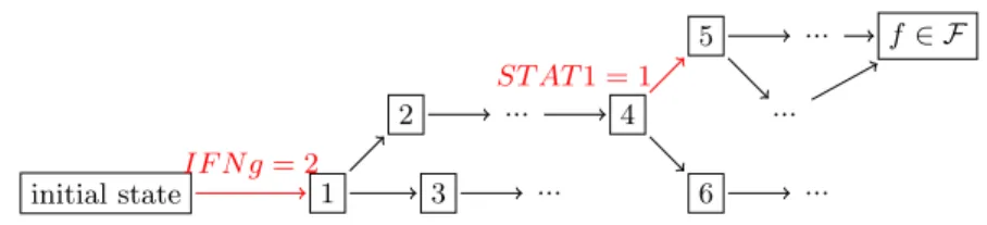
initial state 1 2 3 ... ... 4 5 6 ... ... ... f ∈ F IF N g = 2 ST AT 1 = 1
Fig. 6. Simplification of a perturbation path for T-helper cells
If u ∈ F , Su= {∅}, i.e., no perturbation is necessary. Otherwise, Su consists of the union of Sv for every children v where (u → v) ∈ E and of the union of {l ⊕ s | s ∈ Sv} for every children v where u
l −
→ v ∈ M, and l ⊕ s is the sequence starting with l and followed by s.
To get a minimal set of temporal perturbations, every perturbation sequence that is equal or a superset of initial perturbations are removed, and only the smallest sub-sequences (in terms of sequence inclusion) are kept.
5.2 T-helper cells
We applied a prototype implementation of our algorithm3 on the model of the multi-valued T helper regulatory network introduced in [12].
The initial model has 17 nodes, with 2 or 3 possible values for each. We applied the identification of inevitable reprogramming of the initial state where all the nodes are inactive, except GATA3, IL4, IL4R and STAT6 that have an initial value of 1, to any attractor where Tbet is active, using at most 2 permanent perturbations. The Perturbed Transition Graph has 21,647 nodes, and 20,941 connected components. The set of temporal reprogramming paths uses the following perturbations:
– IFNg=2, then, after several transitions, IFNgR=0 – IFNg=2, then, after several transitions, STAT1=0 – IFNgR=2, then, after several transitions, STAT1=0
The graph in Fig. 6 gives an example of a possible perturbation path that uses INFg=2 and STAT1=0:
From the initial state, a permanent perturbation (INFg=2) is performed. The new perturbed state, 1, has several possible futures, one of which leads to the state 4 in the graph. From this state, the system can continue to follow its usual dynamics, or can be perturbed again with STAT1=1 to go to the state 5, that will always reach the final state. It can be seen that there are branching paths: our method guarantees that from each reachable node there is perturbation path leading to the final state, using one the three perturbation paths given above.
If one applies these perturbations (IFNg=2 and STAT=1) directly in the initial state, the attractor where Tbet is active is not reachable. Therefore, this
3
perturbation path gives a new reprogramming strategy. Moreover, the temporal reprogramming solutions returned by our method are complete.
5.3 Cardiac Gene Regulatory Network
The same algorithm has been applied to the Boolean model of the cardiac gene regulatory network built in [11]. The Boolean network has 15 nodes. Its Per-turbed Transition Graph with at most 3 permanent perturbations has around 60,000 reachable states.
In this example, we computed the fixpoints of the Boolean network and identified reprogramming solutions to change from one fixpoint to another.
For some cases, we observe that temporal reprogramming provides solutions requiring only two perturbations when at least three perturbations are required when applied only in the initial state.
For instance, let us consider the inevitable reprogramming from the fix-point where all nodes are active except Bmp2, Fgf8, Tbx5, exogen BMP2 I, and exogen BMP2 II to the fixpoint where all nodes are inactive but Bmp2, exogen BMP2 I, and exogen BMP2 II. Our method identifies 1 set of 3 pertur-bations to apply in the initial state; and 14 sequences of temporal perturba-tions, one of which requires only 2 perturbations (the loss of function of exo-gen CanWnt I, followed later by the gain of function of exoexo-gen BMP2 I).
6
Discussion
Temporal reprogramming consists in applying perturbations in a specific order and in specific states of the system to trigger and control an attractor change.
This paper establishes the complete characterization of temporal perturba-tions for Boolean networks reprogramming. Perturbaperturba-tions can be applied at the initial state, and during the transient dynamics of the system. This later feature allows to identify new strategies to reprogram regulatory networks, by providing solutions with different targets and possibly requiring less perturbations than when applied only in the initial state.
Our method relies on a Petri net modelling the combination of Boolean net-work asynchronous transitions with perturbation transitions. The identification of temporal reprogramming solutions then relies on a explicit exploration of the resulting state transition graph. Our framework can handle temporary (e.g., through signalling) and permanent (e.g., mutations) perturbations for the exis-tential and inevitable reprogramming to the targeted state.
Future work will focus on increasing the scalability of temporal reprogram-ming predictions. Notably, we aim at using partial order exploration and unfold-ing of the Petri net model in order to exploit the concurrency of transitions.
References
1. W. Abou-Jaoud´e, P. T. Monteiro, A. Naldi, M. Grandclaudon, V. Soumelis, C. Chaouiya, and D. Thieffry. Model checking to assess t-helper cell plasticity. Frontiers in Bioengineering and Biotechnology, 2, 2015.
2. L. Bernardinello and F. De Cindio. A survey of basic net models and modular net classes. In G. Rozenberg, editor, Advances in Petri Nets 1992, volume 609 of Lecture Notes in Computer Science, pages 304–351. Springer Berlin / Heidelberg, 1992.
3. R. Chang, R. Shoemaker, and W. Wang. Systematic search for recipes to generate induced pluripotent stem cells. PLoS Computational Biology, 7(12):e1002300, Dec 2011.
4. C. Chaouiya, A. Naldi, E. Remy, and D. Thieffry. Petri net representation of multi-valued logical regulatory graphs. Natural Computing, 10(2):727–750, 2011. 5. T. Chatain, S. Haar, L. Jezequel, L. Paulev´e, and S. Schwoon. Characterization
of reachable attractors using Petri net unfoldings. In P. Mendes, J. Dada, and K. Smallbone, editors, Computational Methods in Systems Biology, volume 8859 of Lecture Notes in Computer Science, pages 129–142. Springer Berlin Heidelberg, 2014.
6. D. P. A. Cohen, L. Martignetti, S. Robine, E. Barillot, A. Zinovyev, and L. Calzone. Mathematical modelling of molecular pathways enabling tumour cell invasion and migration. PLOS Computational Biology, 11(11):1–29, 11 2015.
7. I. Crespo, T. M. Perumal, W. Jurkowski, and A. del Sol. Detecting cellular re-programming determinants by differential stability analysis of gene regulatory net-works. BMC Systems Biology, 7(1):140, 2013.
8. A. del Sol and N. J. Buckley. Concise review: A population shift view of cellular reprogramming. STEM CELLS, 32(6):1367–1372, 2014.
9. T. Graf and T. Enver. Forcing cells to change lineages. Nature, 462(7273):587–594, dec 2009.
10. R. Hannam, A. Annibale, and R. Kuehn. Cell reprogramming modelled as transi-tions in a hierarchy of cell cycles. ArXiv e-prints, Dec. 2016.
11. F. Herrmann, A. Groß, D. Zhou, H. A. Kestler, and M. K¨uhl. A boolean model of the cardiac gene regulatory network determining first and second heart field identity. PLOS ONE, 7(10):1–10, 10 2012.
12. L. Mendoza. A network model for the control of the differentiation process in th cells. Biosystems, 84(2):101 – 114, 2006. Dynamical Modeling of Biological Regulatory Networks.
13. M. K. Morris, J. Saez-Rodriguez, P. K. Sorger, and D. A. Lauffenburger. Logic-based models for the analysis of cell signaling networks. Biochemistry, 49(15):3216– 3224, 2010. PMID: 20225868.
14. S. Ronquist, G. Patterson, M. Brown, H. Chen, A. Bloch, L. Muir, R. Brockett, and I. Rajapakse. An Algorithm for Cellular Reprogramming. ArXiv e-prints, Mar. 2017.
15. O. Sahin, H. Frohlich, C. Lobke, U. Korf, S. Burmester, M. Majety, J. Mattern, I. Schupp, C. Chaouiya, D. Thieffry, A. Poustka, S. Wiemann, T. Beissbarth, and D. Arlt. Modeling ERBB receptor-regulated G1/S transition to find novel targets for de novo trastuzumab resistance. BMC Systems Biology, 3(1):1–20, 2009. 16. R. Samaga, A. Von Kamp, and S. Klamt. Computing combinatorial
interven-tion strategies and failure modes in signaling networks. Journal of Computainterven-tional Biology, 17(1):39–53, Jan 2010.
17. K. Takahashi and S. Yamanaka. A decade of transcription factor-mediated repro-gramming to pluripotency. Nat Rev Mol Cell Biol, 17(3):183–193, Feb 2016. 18. R.-S. Wang, A. Saadatpour, and R. Albert. Boolean modeling in systems biology:
an overview of methodology and applications. Physical Biology, 9(5):055001, 2012. 19. J. G. T. Za˜nudo and R. Albert. Cell fate reprogramming by control of intracellular