HAL Id: hal-01359995
https://hal.archives-ouvertes.fr/hal-01359995
Submitted on 5 Sep 2016
HAL is a multi-disciplinary open access
archive for the deposit and dissemination of
sci-entific research documents, whether they are
pub-lished or not. The documents may come from
teaching and research institutions in France or
abroad, or from public or private research centers.
L’archive ouverte pluridisciplinaire HAL, est
destinée au dépôt et à la diffusion de documents
scientifiques de niveau recherche, publiés ou non,
émanant des établissements d’enseignement et de
recherche français ou étrangers, des laboratoires
publics ou privés.
Managing temporal allocation in Integrated Modular
Avionics
Nesrine Badache, Katia Jaffres-Runser, Jean-Luc Scharbarg, Christian Fraboul
To cite this version:
Nesrine Badache, Katia Jaffres-Runser, Jean-Luc Scharbarg, Christian Fraboul.
Managing
tem-poral allocation in Integrated Modular Avionics. 19th IEEE International Conference on
Emerg-ing Technologies and Factory Automation (ETFA 2014), Sep 2014, Barcelone, Spain.
pp.
1-8,
�10.1109/ETFA.2014.7005225�. �hal-01359995�
O
pen
A
rchive
T
OULOUSE
A
rchive
O
uverte (
OATAO
)
OATAO is an open access repository that collects the work of Toulouse researchers and
makes it freely available over the web where possible.
This is an author-deposited version published in :
http://oatao.univ-toulouse.fr/
Eprints ID : 15187
The contribution was presented at ETFA 2014:
http://eeyem.eap.gr/en/content/19th-ieee-international-conference-emerging-technologies-and-factory-automation-etfa-2014
To cite this version :
Badache, Nesrine and Jaffres-Runser, Katia and Scharbarg,
Jean-Luc and Fraboul, Christian Managing temporal allocation in Integrated
Modular Avionics. (2014) In: 19th IEEE Internationa l Conference on Emerging
Technologies and Factory Automation (ETFA 2014), 16 September 2014 - 19
September 2014 (Barcelone, Spain).
Any correspondence concerning this service should be sent to the repository
administrator:
[email protected]
Managing temporal allocation in Integrated Modular
Avionics
Nesrine Badache, Katia Jaffr`es-Runser, Jean-Luc Scharbarg and Christian Fraboul University of Toulouse
IRIT-INPT/ENSEEIHT
2, rue Charles Camichel, 31000 Toulouse, France
{nesrine.badache, katia.jaffresrunser, jean-luc.scharbarg, christian.fraboul}@enseeiht.fr
Abstract—Recent civil airborne platforms are produced using Integrated Modular Avionics (IMA). IMA promotes both sharing of execution and communication resources by the avionics appli-cations. Designs following IMA decrease the weight of avionics equipment and improve the whole system scalability. However, the price to pay for these benefits is an increase of the system’s complexity, triggering a challenging system integration process. Central to this integration step are the timing requirements of avionics applications: the system integrator has to find a mapping of applications and communications on the available target architecture (processing modules, networks, etc.) such as end-to-end delay constraints are met. These challenges stress the need for a tool capable of evaluating different integration choices in the early design stages of IMA.
In this paper, we present and formalize the problem of spatial and temporal integration of an IMA system. Then, we focus on the temporal allocation problem which is critical to ensure a proper timely behavior of the system. Two main properties are presented to ensure perfect data transmission for hard real-time flows. To quantify the quality of a set of valid temporal allocations, CPM utilization and communication robustness performance criteria are defined. We show on an example that both criteria are antagonist and that they can be leveraged to choose an allocation that either improves the system computing performance or the robustness of the network.
I. INTRODUCTION
Embedded avionics systems have evolved from a federative architecture where calculators dedicated to avionics appli-cations were interconnected through dedicated mono-emitter links towards a modular and distributed architecture.
An IMA architecture interconnects several spatially dis-tributed processing units, sensors and actuators using one or more communication networks. Processing units communicate most of the time using an AFDX network (Avionic Full Duplex Switched Ethernet) which has been standardized in ARINC 664 [3]. Avionics applications are distributed over the set of processing units called core processing modules. Current integration choices are made thanks to the experience and know-how of specialists. These specialists have limited tools to guide such a complex and crucial design process. However, such systems encompass around a hundred CPMs, exchanging a thousand of flows. This magnitude clearly calls for a guided design and integration process.
In the literature, only few works have proposed solutions to the IMA integration problem. Lauer et al. [6] have modeled
the IMA architecture using formal methods and calculated worst case network traversal times using trajectory approach to verify the timing requirements of the whole system. This ap-proach has scalability issues as it relies on formal verification. Al Sheikh et al. [9] propose a mixed integer linear program to optimize the spatial and temporal integration choices with resource constraints. Solutions obtained with this approach are unfortunately not robust to the asynchronism of the modules. More specifically, the calculated solution holds for a set of module startup offset, but may not work anymore for a different set of offsets. Moreover, the approach does not scale up to the size of future larger IMA architectures.
The work presented herein is a step ahead of our previous studies presented in [10] and [7]. This paper focuses on the derivation of the execution period of partitions which are receiving time-constrained data from distant source partitions. The proposed approach completely mitigates message losses for all flows in the network by introducing two constraints on the end-to-end communication delay. We show that several allocations meet these constraints and that it is not always obvious to decide which solution is the most interesting one for the system integrator.
The paper is organized as follows. Section II introduces the IMA integration issues while Section III relies on a worst case analysis to define the constraints that ensure failure-free message deliveries. Section IV illustrates these constraints on a practical example and exhibits the need for a more precise performance evaluation. Next, Section V introduces CPM utilization and communication robustness criteria. Finally, Section VI concludes this paper.
II. IMAINTEGRATION ISSUES
A. Integrated Modular Avionics (IMA)
The Integrated Modular Avionics (IMA) architecture has been developed in the late 2000s for civil avionics systems. It has been standardized as ARINC 651 [1] for the definition of the generic hardware architecture and as ARINC 653 [2] for the corresponding software architecture. The design goal of the software architecture, called APEX (APplication EXecutive interface), is to enable spatial and temporal partitioning of the avionics functions for the target architecture.
IMA is a distributed architecture where processing units, called Core Processing Modules (or CPM) are interconnected through embedded communication networks. An avionics ap-plication is composed of a set of functions or tasks which may be executed on a single or on several CPMs, distributively. In this latter case, two tasks executed on two distant CPMs communicate through the so-called APEX communication ports to create an APEX logical channel. These APEX ports are reminiscent of standard IP world sockets. Logical ports are mapped to a physical interface of the underlying communica-tion network.
To ensure physical and temporal segregation of memory and computing resources, a static resource allocation of the avion-ics tasks is enabled by APEX. APEX defines an execution time window that repeats periodically on a CPM to execute a set of tasks grouped in partitions. A partition Piis characterized
by its execution duration biand its period Ti. A set of tasks is
assigned by the integrator to a partition. Consequently, this set of tasks is executed with the periodicity of the hosting partition and their total execution duration is bounded by the duration of the hosting partition as well. The set of all partitions hosted on the same CPM are scheduled in a cyclical frame called MAjor
time Frame(MAF). The length of a MAF is given by the least common multiple of the partition periods. Several instances of the same partition may be executed within a MAF.
Each partition is assigned a dedicated and reserved memory and computing space used for both data storage and execution. Thus, the tasks assigned to two different partitions can not access the same memory space.
Two distant communicating tasks belong to two distinct communicating partitions. A communication is unidirectional, with one source partition and one destination partition. Data are emitted periodically, following the source partition execu-tion period.
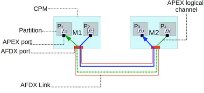
Fig. 1. IMA integration example
Figure 1 pictures a toy example of an IMA system com-posed of two CPMs, hosting two partitions each. In each partition, only one task is being executed. Tasks fB and fA
(resp. fC and fD) belong to the same avionics application.
fB emits data to fA using its emission APEX port, which
is mapped to an AFDX virtual link (the dotted green line) connected to the receiving partition P1, hosting function fA.
Similarly, fC emits to fD using another AFDX virtual link
(in solid blue). Figure 2 represents a possible MAF of the
first CPM hosting the two partitions P1and P2. As illustrated,
partition P1repeats with period T1
Fig. 2. MAF illustration
B. IMA design and integration issues
Given a target architecture described by the layout of CPMs and networks, and a set of applications (e.g., flight warning, automatic cruise control, etc.), the integration process has to solve several problems. The first problems are related to the physical allocation of the applications to the available CPMs and networks. It decomposes into two main steps:
The spatial allocation of applications to CPMs. An avionics application is first segmented into a set of partitions hosting its processing functions. Each partition has to be assigned to a CPM knowing that each CPM has an available memory space budget and a given processing speed.
The spatial allocation of APEX logical channels to networking resources. If an application is deployed over several CPMs, their functions communicate via the network using APEX channels. The APEX logical channels defined between the distant applications have to be mapped to the available communication channels provided by the embedded networks of the target architecture (i.e. AFDX virtual links, ARINC 429 links, etc.).
Once a possible spatial allocation of the applications is set, the integrator knows on which CPMs each partition of each ap-plication runs. He knows as well which worst case networking latencies are expected between two communicating partitions [12], [11]. The data emitted by each source partition is timely constrained by a freshness parameter (F P ). Once the data leaves the output APEX port of a partition, a counter is armed. The data has to be consumed by its destination partition before this freshness duration has elapsed. This constraint has to be ensured for each set of communicating partition. To meet these constraints and accept the possible spatial allocation under study, a valid temporal allocation of the destination partitions periods has to be found, which is discussed next.
Temporal period allocation of destination partitions. Since the applications set the period of the source partitions, only the period of destination partitions can be tuned by the system integrator to ensure proper message delivery between the two communicating partitions. The destination period can be adjusted to compensate for possible jitters introduced by the network. Moreover, as explained above, allocated partitions on each CPM are grouped into a MAF, which is given by the least common multiple of the partition periods. Thus, by allocating periods of destination partitions, the MAF is modified as well. This paper concentrates on the temporal allocation of parti-tions. These temporal integration issues are complex to solve
for current avionics systems which are typically composed of more than a hundred of CPMs, interconnected by thousands of virtual links. To tackle this problem, we introduce first two specific constraints that ensure, knowing the worst case communication delay, that no data is lost for a given partition-to-partition communication. Then, we illustrate on an example that several temporal allocations meet these constraints. To characterize the efficiency of these admissible solutions, we introduce two performance criteria that measure the delay margin of the flows and the MAF occupancy percentage. The intuition behind these criteria is to be able to select solutions which are more robust to a possible future increase in network jitters or to select solutions which provide room for adding new partitions in the CPMs. Proposed criteria could be combined in the future to extract solutions that trade-off both metrics, using a multi-objective optimization heuristic.
III. TEMPORAL PERIOD INTEGRATION:WORST CASE ANALYSIS
This section defines first the IMA system model we con-sider, and then recalls the precise definition of the end-to-end functional delay of [6]. This delay is the partition-to-partition communication delay which is constrained by the freshness parameter introduced previously. Next, two constraints on the destination period are introduced that ensure perfect message receptions for a partition to partition communication. We prove that if a temporal period allocation fulfills these two constraints, no message can be lost.
A. IMA system model
An avionics application is represented in the following as a setP = {P1,...,Pn} of partitions that have to be allocated and
scheduled on a setM = {M1,...,Mm} of parallel CPMs. Each
partition Pi ∈ P is characterized by the number of functions
it hosts. In this work, we assume that one partition hosts one and only one function. Formally, partition Pi is defined by its
execution period Ti and duration bi. We define with dn the
date of the nth partition activation.
In its partition, we assume a function f first reads the messages coming from one or more source functions (source functions may be distant or local), then processes its data and at the end of bi, sends its messages on the APEX port. Function
f is characterized by its worst case execution time. Since we assume that a partition only hosts one function, its worst case execution time is equal to the duration bi of the partition Pi
it belongs to.
IMA system is completely distributed: CPMs have different start-up dates. These different start-up dates are modeled by relative offsets. The offset of CPM Mℓ is denoted by φℓ
(cf. Fig. 2).
The communication between a source partition Pi and a
destination partition Pj is defined as an APEX logical
chan-nels denoted Comi,j. Comi,j is constrained by a freshness
parameter F Pi,j. We recall that it is the maximum time a
message can wait before being consumed at the destination function from its emission date at the source APEX port.
B. End-to-end functional communication delay
We consider a communication Comi,j represented in
Fig-ure 3 between a sender partition Piallocated on CPM Mℓ, and
a destination partition Pj allocated on CPM Mk. The source
partition Pi emits periodically, at the end of its execution
duration, an occurrence of the message flow msg that must be read at the next activation of Pj. The nth occurrence of
the flow msg is denoted by msgn.
The end-to-end functional communication delay [6] is the sum of the following latencies as illustrated in Fig. 3:
• SOURCE BUFFERING LATENCY: A message occurrence msgngenerated by a sensor connected to the module Mℓ
may have to wait for the source partition Pi to be active
before being consumed in the buffer.
• SOURCE EXECUTION DURATION: Partition Pi is active
for biunits of time. During this source execution duration,
msgn stays at the source partition until it is sent to the
APEX output port.
Fig. 3. End-to-end functional and communication delays
• NETWORK LATENCY : Each occurrence msgn
experi-ences a network latency denoted by Li,j on its
communi-cation channel Comi,j. We assume here that this latency
Li,j belongs to the interval [Lmin, Lmax], where Lminis
the best case network latency and Lmaxis the worst case
network latency on Comi,j. The network latency on each
APEX logical channel is bounded which is compatible with well-know worst case calculation studies done in the context of avionics embedded networking [11], [12]. Notice that Lmin and Lmaxdepend as well on indices i
and j but for clarity purposes, they have been omitted in this paper.
• DESTINATION LATENCY : Once msgn arrives at the
destination CPM, it may have to wait for the partition Pj to become active and being read by the destination
function. The duration between the date msgn arrives
at Mk and the date it is consumed by Pj is defined
as the destination latency. The occurrences msgn that
are received at the destination partition do not constitute a periodic flow anymore. This is a consequence of the variable network latency and the difference in start-up dates of CPMs.
• DESTINATION EXECUTION DURATION: Once msgn is
received by Pj, it is processed for a duration of bj units
We define herein as well the end-to-end communication
delay(denoted as E2Ei,j) which is the sum of the network and
destination latencies as shown on Fig. 3. This latency is the one which has to be lower or equal than the freshness parameter F Pi,j for msgn to be considered as valid. The end-to-end
communication delay is central for the derivations proposed in the rest of this paper.
C. Worst case destination period analysis
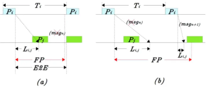
Considering these different latencies and variabilities in the end-to-end communication delay, two constraints on the destination partition periods are introduced that ensure a timely and failure free message delivery.
A message occurrence msgn can be lost for two reasons: • msgn experiences an end-to-end communication delay
larger than F Pi,j (cf. Fig. 4-(a)),
• msgnis overwritten by msgn+1before being read by Pj
(cf. Fig. 4-(b))
Occurrence msgn is overwritten by msgn+1 if the two
following conditions occur: i) msgn arrives too late to be
consumed by the activation of Pj immediately following the
activation of Pi (in this case, it has to wait an extra period
Tj for the next activation of Pj) and ii) if during this extra
waiting time, a newer occurrence msgn+1 arrives at Pj and
overwrites msgn in the destination buffer.
To sum-up, message losses may occur if the resulting end-to-end communication delay is greater than the required freshness parameter F Pi,j), or if an other occurrence msgn+1
is received before the consumption of msgn.
Fig. 4. Piand Pjcommunication
To avoid such losses of messages, the destination execution period Tj of Pjhas to be adjusted so that these two loss cases
never happen. We show next that these requirements are met if following Properties 1 and 2 hold:
Property 1. A message does not violate its freshness
param-eter F Pi,j if and only if:
Tj≤ F Pi,j− Lmax (1)
Proof:
In order to meet the freshness constraint F Pi,j associated to
Comi,j, the end-to-end communication delay of the message
msgn, denoted E2En must not exceed F Pi,j:
E2En≤ F Pi,j
By definition, we have:
Li,j+ Ji,j ≤ F Pi,j
In the worst case, Li,j is equal to Lmaxand msgnhas to wait
an entire period Tj(e.g. msgnarrives just after the destination
partition has been activated). Thus, Ji,j is equal to Tj in the
worst case and:
Lmax+ Tj≤ F Pi,j (2)
From Eq. (2), it can be deduced that if the destination period exceeds F Pi,j− Lmax, the freshness constraint is not met for
msgn. In other words, valid values of Tj have to follow:
Tj≤ F Pi,j− Lmax
If partition Pj is the destination partition of K different
source partitions, its period Tj has to be adjusted considering
the most restrictive freshness parameter among the K required ones. In this case, Property 1 holds by replacing F Pi,j with
mink(F Pk,j).
Property 2. A message msgnis never overwritten by a newer
occurrence msgn+1 if and only if
Tj < Ti− (Lmax− Lmin) (3)
The destination period Tj has to be reduced to prevent the
reception of two occurrences of msg between two successive executions of Pj.
Fig. 5. Minimal execution period
Proof:
Two successive occurrences of msg, msgn and msgn+1,
are sent by Pi.
Occurrences msgn and msgn+1 should respectively be
received at the destination partition Pj at the dates dn (the
nth activation of P
i) and dn+1 (the (n + 1)th activation of
Pi). These dates are defined by:
dn= φℓ+ nTi+ bi+ Ln
dn+1= φℓ+ (n + 1)Ti+ bi+ Ln+1
where Lnand Ln+1are the network latencies experienced by
msgn and msgn+1, respectively.
The destination partition Pjreads both occurrences of msg
if the destination period Tj follows:
After substituting dn+1and dnwith their definition, we have:
Tj 6Ti+ Ln+1− Ln
The destination period has to mitigate messages losses for the must constraining case. This case happens for the smallest possible value of dn+1− dn, i.e. the smallest possible value of
Ti+ Ln+1− Ln. This smallest value is experienced if Ln=
Lmax and Ln+1= Lmin. Thus:
Tj6Ti+ Lmin− Lmax
⇔ Tj6Ti− (Lmax− Lmin)
If partition Pj is the destination partition of K different
source partitions, the most constraining communication is the one with the smallest period Ti. Thus, Property 2 holds in this
case by replacing Ti withmink(Tk).
Fig. 6. Oversampling of Pj period
The two properties are combined by setting a maximum possible destination period equal to the minimum of the constraints imposed by Property 1 and 2. In other words,
Tj6Tjmax (4)
with Tmax
j = min (F Pi,j− Lmax, Ti− (Lmax− Lmin)).
To conclude, any value of Tjsmaller than T Pjmaxis a valid
setting where no message occurrences can be lost. As we will show in the next example, if small values of Tj that meet
Eq. (4) are chosen, some activations of Pj may never receive
any message occurrence. Thus, destination period adjustment comes at the price of overusing the CPM at the destination as already noticed in [8] for the FlexRay network static segment configuration. Another drawback is that there is as well less room for adding other partitions to the destination MAF. However, this oversampling has a beneficial effect: if the network jitter increases (i.e. Lmax increases) because of some
evolution in the network load, the current temporal allocation is still robust enough to mitigate occurrence losses due to this increase of Lmax. Both effects will be illustrated on an
example in the next Section.
IV. IMATEMPORAL ALLOCATION EXAMPLE
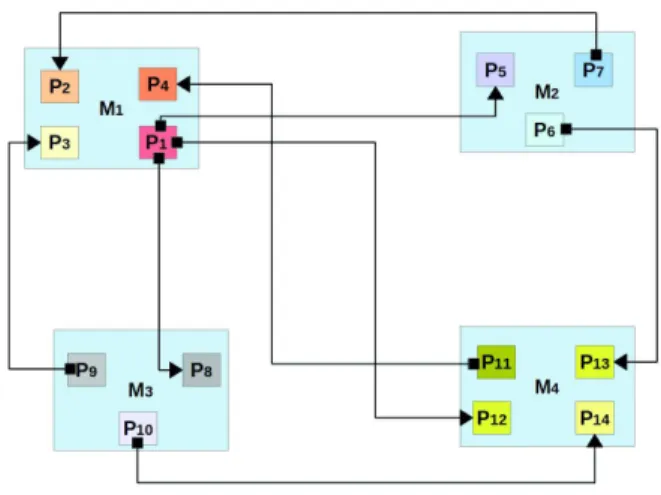
The temporal allocation problem is illustrated on the ex-ample of Fig. 7. It represents the spatial allocation of an application on four CPMs M1, . . . , M4 interconnected by an
AFDX network. We consider that this application is part of
Fig. 7. Example of IMA system
a much larger IMA system which includes other modules hosting other avionics applications.
The application under study decomposes into 14 partitions. As shown in Fig. 7, there are 6 source partitions: P1executes
on CPM M1, P6 and P7 on M2, P9 and P10 on M3, P11 on
M4. Execution periods of these source partitions are imposed
by the application. They are listed in Table I.
Periods Ti(ms) BAG (ms) Destination
P1 120 64 P5, P8, P12 P6 60 32 P13 P7 60 32 P2 P9 60 32 P3 P10 60 32 P14 P11 40 32 P4 TABLE I
SOURCE PARTITION FEATURES
As stated previously, a source partition generates one mes-sage occurrence at the end of each of its execution. These occurrences are transmitted to at least one destination par-tition via an AFDX virtual link. An AFDX virtual link is characterized by its Bandwidth Allocation Gap (BAG) which is the minimum authorized duration between two consecutive message transmissions on the link. In Table I, the BAG of the virtual links are set to be no greater than the period of their corresponding source partitions. Thus, it follows that a message occurrence can never be delayed because of the BAG of its corresponding virtual link. Table I lists as well the destination partitions of each source partition.
The execution duration of all the partitions are given in Table II. Each partition can be activated more than one time in the MAF of its CPM.
The temporal destination period allocation of this configura-tion has to meet the constraints presented in Secconfigura-tion III which are conditioned by the network latency variability (Lminand
Lmax) and the freshness parameter F P . These values for our
Execution durations bi(ms) P1 5 P2 10 P3 10 P4 5 P5 15 P6 15 P7 15 P8 15 P9 15 P10 15 P11 10 P12 10 P13 10 P14 10 TABLE II
EXECUTION DURATIONS OF THE PARTITIONS
Lmin(ms) Lmax (ms) Freshness F Pi,j(ms)
Com1,5 2 12 100 Com1,8 3 15 100 Com1,12 1 6 100 Com6,13 1 6 60 Com7,2 2 12 60 Com9,3 4 20 60 Com10,14 2 10 60 Com11,4 1 5 40 TABLE III
LATENCIES AND FRESHNESS CONSTRAINTS
Thanks to Properties 1 and 2, the maximum allowed desti-nation period Tjmax has to be calculated for each destination
partition following Eq. (4). Let’s detail this computation on partition P5 whose source partition is P1. From Property 1,
we have:
T5 < F P1− Lmax1
< 100 − 12 < 88 ms From Property 2, we have:
T5 < T1− (Lmax1 − Lmin1 )
< 120 − (12 − 2) < 110 ms
Thus, the period of P5 must be equal to at most T5max =
88 ms. Results for other destination partitions are given in Table IV which lists the maximum allowed period to meet Property 1, 2 and both at the same time.
The following step consists in building the MAFs associated to each CPM by choosing the periods of the destination partitions. The destination partitions periods have of course to be lower than Tmax
j but to simplify the scheduling inside
the MAF and keep MAFs to a limited size, partition periods are chosen to be harmonic as well. For each CPM, a solution is given by the set of destination partition periods that respect these constraints (we recall source partition periods are set and can not be changed). Several solutions may fulfill these constraints of course. Tmax j Property 1 Property 2 P2 48 48 50 P3 40 40 44 P4 35 35 36 P5 88 88 110 P8 85 85 108 P12 94 94 115 P13 54 54 55 P14 50 50 52 TABLE IV
DESTINATION PARTITION CONSTRAINTS
In our example, following solutions are chosen per CPM:
• For module M2, source partitions P6 and P7 have a
period of 60 ms. We recall that destination partition period T5must not exceed 88 ms. Thus, one valid solution
is to assign a period of 60 ms to the three partitions.
• The same assignment can be done for partitions P8, P9
and P10on module M3,
• For module M4, a similar reasoning leads to a period of
40 ms for partitions P11, P13 and P14, and to a period
of 80 ms for P12. The larger period of 80 is chosen for
P12because T12max= 94 ms and 80 is the largest allowed
value which is harmonic with T11= 40 ms. Choosing a
lower period for P12is possible, but it clearly wastes too
much processing time at M4.
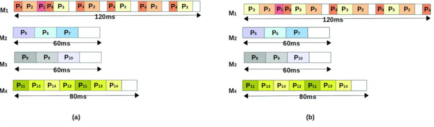
• The case of module M1is a bit more complex. The period
of source partition P1is set to 120 ms by the application,
while periods of P2, P3 and P4 can not exceed 48 ms,
40 ms and 35 ms, respectively. Thus, two solutions are possible:
1) P2 and P3 are assigned a period of 40 ms and P4
a period of 20 ms,
2) P2, P3and P4are assigned a period of 30 ms.
Overall, it leads to two different period assignments on M1
(which are not the only ones possible). Figure 8 shows that both assignments lead to schedulable partitions on CPMs by representing the MAFs obtained for each CPM. The main question raised by this example is how to choose between both valid allocations of CPM M1. This question is discussed
next.
V. PERFORMANCE EVALUATION CRITERIA FOR TEMPORAL ALLOCATION
A. Analysis of the valid allocations for M1
Looking more closely at the MAFs of Fig. 8, it can be seen that the MAF obtained with the first allocation pro-posed for M1 (i.e. where (T2, T3, T4) = (40, 40, 20)) has
more idle space than the one of the second allocation (i.e. where (T2, T3, T4) = (30, 30, 30)). For both solutions, the
same number of message occurrences have to be absorbed by the partitions hosted on M1, thus, allocation 1 uses the
computation power more efficiently than allocation 2. Another analysis perspective is to look at the networking performance. There are three communications ending at M1:
Fig. 8. Two possible integrations in M1
Com7,2, Com9,3 and Com11,4. For each communications, it
is possible to calculate theirs worst case end-to-end commu-nication delay (E2Ewc) which is the sum of their Lmaxvalue
and the destination period chosen either with allocation 1 or allocation 2.
E2Ewc(ms) Freshness F Pi,j(ms) Delay margin
Com7,2 52 60 8
Com9,3 60 60 0
Com11,4 25 40 15
TABLE V
WORST CASEE2EDELAY,FRESHNESS PARAMETER AND DELAY MARGIN FOR COMMUNICATIONS ENDING INM1WITH(T2, T3, T4) = (40, 40, 20).
For instance, for Com7,2 using allocation 1, we have
Lmax = 12 ms and T2 = 40 ms. Thus, E2Ewc = 52 ms.
Still for Com7,2, using allocation 2 this time, T2= 30 ms and
E2Ewc= 42 ms. Compared to the required freshness
param-eter, allocation 2 provides a larger end-to-end communication delay margin than allocation 1 for Com7,2. The same analysis
has been done for the other communications ending at M1and
results can be found in Tables V and VI, for allocations 1 and 2 respectively.
E2Ewc(ms) Freshness F Pi,j(ms) Delay margin
Com7,2 42 60 18
Com9,3 50 60 10
Com11,4 35 40 5
TABLE VI
WORST CASEE2EDELAY,FRESHNESS PARAMETER AND DELAY MARGIN FOR COMMUNICATIONS ENDING INM1WITH(T2, T3, T4) = (30, 30, 30).
From Tables V and VI, it can be seen that the delay margin for allocation 2 is larger in average than for allocation 1. Moreover, the smallest delay margin of allocation 1 is of 0 ms while the smallest one for allocation 2 is of 5 ms. Clearly, allocation 2 provides a better networking performance than allocation 1. If for some reason the network configuration has to be modified, and if this introduces an increase of Lmax of
at most 5 ms per VL, we can conclude that allocation 2 is still valid and no changes in the MAFs have to be made.
Thus, even though allocation 1 has a more efficient use of the CPM computation power, it is less robust from the net-working performance point of view. Both allocations represent two different trade-off between network robustness and CPM utilization. To capture these two features, we propose next to introduce two performance criteria that can be leveraged for a future IMA system-wide multi-objective optimization.
B. CPM utilization factor and communication robustness
This Section defines two performance evaluation criteria capturing the two previously introduces features for a given temporal period allocation:
• CPM utilization factor Qi:For a CPM Mi, the utilization
factor is defined as the percentage of time the CPM is executing a partition. For instance, in Fig. 8, M2and M3
have a utilization factor of 0.75 each. Formally:
Qi=
P
Pk∈Mibk
bM AF
(5)
where bM AF is the MAF duration.
• Communication robustness δi,j:For each communication,
we calculate the margin between the worst case end-to-end communication delay and its corresponding freshness parameter. If this margin is very small, any change in the network configuration may lead to losses and the whole system may have to be re-designed. Formally:
δi,j = F Pi,j− E2Ewc= F Pi,j− (Lmax+ Tj) (6)
C. System-wide metrics
The previously defined elementary metrics measure either the performance of an allocation at the CPM level or at the communication level. It is useful to define a metric to characterize the global performance of the whole IMA system under study. Several options are possible and we introduce two of them.
In the first option, it possible to define a global metric by
averagingthe elementary metrics. Global average metrics are formally defined by:
Global average CPM utilization factor Qavg:
Qavg= P
i∈[1..m]Qi
m (7)
with m is the number of CPMs in the system. Global average communication robustness∆avg:
∆avg=
P
(i,j)δi,j
ncom
(8)
where ncom is the number of communications in the system.
Another option is to select the worst elementary metric as representative of the system performance. In this case, the global metrics are given by:
Global worst CPM utilization factor Qw:
Qw= max
i∈[1..m]Qi (9)
Global worst communication robustness∆w:
∆w= min
(i,j)δi,j (10)
For the communication robustness, it is in our opinion more interesting to use the global∆wmetric compared to the
average one because it clearly identifies the communication that may be detrimental to the overall performance. On the contrary, for the CPM utilisation, we are more interested in the average load of the system and the peak load.
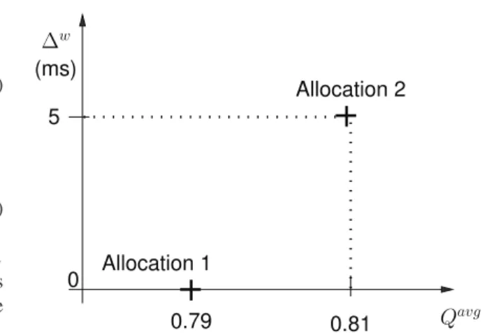
It is possible to illustrate the global metrics Qavg and∆w
for allocations 1 and 2 on the previous example. For alloca-tion 1, Qavg = 0, 79 while for allocation 2, Qavg = 0, 81.
The system-wide CPM utilization criteria clearly shows that allocation 1 is more efficient than allocation 2.
Looking at the communication robustness, ∆w= 0 ms for
the first allocation. This very small global margin is caused by Com9,3. For allocation 2, ∆w = 5 ms. It is communication
Com11,4that experiences a margin of 5. This criteria clearly
shows that allocation 2 has a better communication robustness, which is in line with our previous analysis. The performance of both allocations is illustrated in the 2-dimensional space of (Qavg,∆w) in Fig. 9. The best trade-off is obtained for low
values of Qavg and high values of∆w.
To conclude, we have illustrated these metrics on a small-scale example. In practice, more than thousands of flows and hundreds of CPMs are embedded into an avionics IMA platform. Thus, managing the temporal allocation is a very large and complex problem. There is a clear need for an auto-mated help for the design of such systems. In this paper, we have analyzed the temporal allocation problem and provided system-wide performance analysis criteria. These criteria can now be leveraged to optimize the temporal allocation problem. Since both CPM utilization and communication robustness criteria are antagonist by nature, multi-objective optimization can be addressed to provide different trade-off solutions to the system integrator. ∆w Qavg 0.79 Allocation 1 0 5 0.81 Allocation 2 (ms)
Fig. 9. Multi-objective performance of allocation 1 and 2 for (Qavg,∆w).
VI. CONCLUSION
In this paper, the issues related to the spatial and temporal integration of an IMA system are introduced. For the temporal period allocation problem, two main properties have been proved that ensure perfect data transmission for all time-constrained flows of the system. Next, we have proposed two criteria, naming CPM utilization and communication robustness, to quantify the quality of valid temporal allo-cations. All these contributions have been illustrated on a practical example. Future works will concentrate on defining and solving a multi-objective optimization problem leveraging the performance criteria presented in this paper.
REFERENCES
[1] Aeronautical Radio Inc. ARINC 651, Design Guidance for Integrated
Modular Avionics, 1991.
[2] Aeronautical Radio Inc. ARINC 653, Avionics Application Software
Standard Interface, 1997.
[3] Aeronautical Radio Inc. ARINC 664, Aircraft Data Network, Part 7:
Avionics Full Duplex Switched Ethernet (AFDX) Network, 2005. [4] Aeronautical Radio Inc. ARINC 429, ARINC specification 429-ALL:
Mark 33 Digital Information Transfer System, 2001.
[5] Lauer, M. and Ermont, J. and Boniol, F. and Pagetti, C. : Latency and
freshness analysis on IMA systems. 16th IEEE International Conference on Emerging Technologies and Factory Automation, Toulouse, France, September 2011
[6] Lauer, M. and Ermont, J. and Boniol, F. and Pagetti, C. : Analyzing
end-to-end functional delays on an IMA platform. In Proc. of the 4th ISoLA’10, Heraklion, Greece, page 243-257. Springer-Verlag, 2010. [7] N. Badache, K. Jaffres-Runser, J.-L. Scharbarg,C. Fraboul : End-to-end
delay analysis in an Integrated Modular Avionics architecture. (short paper)ETFA 2013, Cagliari, Italy, Sep. 2013.
[8] M. Grenier, L. Havet, N. Navet : Configuring the communication on
FlexRay- the case of the static segment. 4th European Congress on Embedded Real Time Software, Toulouse, France, January 2008. [9] A. Al Sheikh and al. : Partitions scheduling on an IMA platform with strict
periodicity and communication delaysRTNS 2010, Toulouse, France. [10] F. Martin and C. Fraboul : Modeling and Simulation of Integrated
Modular Avionics Parallel and Distributed Processing. Proceedings of the Sixth Euromicro Workshop, Madrid, Spain, January 1998. [11] Bauer, H. and Scharbarg, J. and Fraboul, C : Improving the Worst-Case
Delay Analysis of an AFDX Network Using an Optimized Trajectory ApproachIEEE Transactions on Industrial Informatics 2010, pages 521-533.
[12] Charara, H. and Scharbarg, J. and Ermont, J. and Fraboul, C. : Methods
for bounding end-to-end delays on an AFDX network 18th Euromicro Conference on Real-Time Systems, Dresden, Germany, July 2006.