Classifying superheavy elements by machine learning

Classifying superheavy elements by machine learning

The MIT Faculty has made this article openly available. Please share

how this access benefits you. Your story matters.

Citation

Gong, Sheng et al. "Classifying superheavy elements by machine

learning." Physical Review A 99, 2 (February 2019): 022110 © 2019

American Physical Society

As Published

http://dx.doi.org/10.1103/PhysRevA.99.022110

Publisher

American Physical Society

Version

Final published version

Citable link

http://hdl.handle.net/1721.1/120709

Terms of Use

Article is made available in accordance with the publisher's

policy and may be subject to US copyright law. Please refer to the

publisher's site for terms of use.

Classifying superheavy elements by machine learning

Sheng Gong,3,2Wei Wu,2Fancy Qian Wang,1,2Jie Liu,1,2Yu Zhao,2Yiheng Shen,1,2Shuo Wang,2 Qiang Sun,2,1,*and Qian Wang1,2,†

1_{Center for Applied Physics and Technology, BKL-MEMD, College of Engineering, Peking University, Beijing 100871, China} 2_{Department of Materials Science and Engineering, College of Engineering, Peking University, Beijing 100871, China} 3_{Department of Materials Science and Engineering, Massachusetts Institute of Technology, Cambridge, Massachusetts 02139, USA}

(Received 4 December 2018; published 8 February 2019)

Among the 118 elements listed in the periodic table, there are nine superheavy elements (Mt, Ds, Mc, Rg, Nh, Fl, Lv, Ts, and Og) that have not yet been well studied experimentally because of their limited half-lives and production rates. How to classify these elements for further study remains an open question. For superheavy elements, although relativistic quantum-mechanical calculations for the single atoms are more accurate and reliable than those for their molecules and crystals, there is no study reported to classify elements solely based on atomic properties. By using cutting-edge machine learning techniques, we find the relationship between atomic data and classification of elements, and further identify that Mt, Ds, Mc, Rg, Lv, Ts, and Og should be metals, while Nh and Fl should be metalloids. These findings not only highlight the significance of machine learning for superheavy atoms but also challenge the conventional belief that one can determine the characteristics of an element only by looking at its position in the table.

DOI:10.1103/PhysRevA.99.022110 I. INTRODUCTION

Elements can be classified into metals, metalloids, and nonmetals according to their overall chemical properties [1–4]. Among the discovered 118 elements [5], 85 of them are classified as metals, 17 are classified as nonmetals, and seven are classified as metalloids [1,2,4,6,7], as shown in Fig. 1. However, for the superheavy elements with atomic number (Z) greater than 108, at present only Cn (Z= 112) has been experimentally classified as a metal [8,9]. Although experiments have also been conducted for the chemistry of Nh (Z = 113) and Fl (Z = 114), the results and conclusions are uncertain and even contradictory to each other [9–14]. Due to the limitations associated with half-life and production rate, the chemistry of other superheavy elements has not been experimentally studied. How to classify such superheavy elements has been a long-standing question.

Theoretical study of molecules or crystals containing su-perheavy elements by using relativistic quantum mechanics (RQM) is challenging [15–19], and in many cases the pre-dictions are contradictory to each other [1,10–12], and/or inconsistent with experiments [9–11,18,20]. Therefore, it is necessary to use alternative predictive methods for these superheavy elements. The atomic properties derived from RQM are considered to be more reliable as such calculations have more secure theoretical foundation [15–17,19], where different methods usually can generate quite similar results [17,21] that are in agreement with experiments [17,20–22]. However, classifying elements by atomic properties remains an unsolved problem. Although some quantities like first ion-ization energy and electronegativity are related to the metallic

*_{sunqiang@pku.edu.cn} †_{qianwang2@pku.edu.cn}

behavior of elements [2,3], there exist many irregularities [3,23], especially in the region of transition metals due to the nature of d-orbital radial distributions [24]. To overcome these problems, multicriterion descriptions were proposed [1,4], and the parameters for the aggregates of atoms were also included in these schemes in addition to atomic properties. However, to the best of our knowledge, there is no study reported thus far to classify elements with high accuracy solely by atomic properties, which motivates us to carry out this study by using machine learning (ML), a very powerful tool for classification as it can discover complex predictive relations among multiple variables. In fact, ML has received considerable attention currently with significant progresses in academic and commercial applications such as health care, manufacturing, and finance [25]. Especially, ML has recently been employed for solving classification problems in physics and chemistry including high or low spin state of transition-metal complexes [26], metal or insulator in half-Heusler com-pounds [27], and failures or successes in chemical reactions [28]. However, most of the current ML schemes used for physics rely on the properties of aggregates of atoms as input, which prohibits their application for superheavy elements. In this paper we train ML classifiers (decision tree [29] and support vector machines [30]) based solely on atomic data to directly tackle two aforementioned problems: (1) employing ML to find the relationship between atomic properties and classification of the elements and (2) using the trained classi-fiers with high accuracy to classify those superheavy elements without known labels.

II. RESULTS AND DISCUSSIONS

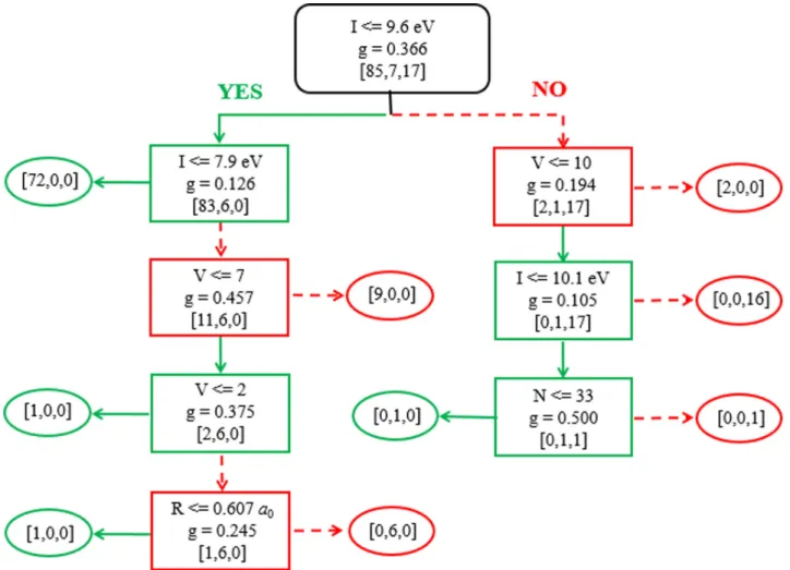
To gain an overview of the data set, we train a human-interpretable decision tree classifier as shown in Fig. 2, in

SHENG GONG et al. PHYSICAL REVIEW A 99, 022110 (2019)

FIG. 1. Classification of elements in the periodic table. Color coding: yellow, metal; gray with underlined symbol, metalloids; blue in bold and italic symbol, nonmetal; white, elements with unknown classification.

which the data are partitioned into branches and leaves based on the concept of information impurity [31]. One can see that only one class exists in each leaf node, indicating that

the decision tree classifier can achieve 100% accuracy in the training set. Furthermore, to quantitatively study the signifi-cance of each feature used in the classification, we derive the

FIG. 2. Decision tree classifier trained for all elements with known classification. Rectangles represent decision nodes, and ovals represent leaf nodes. I, first ionization energy; V, number of valence electrons; R, atomic radius; N, atomic number; g, Gini coefficient [31]; the three numbers from left to right in the square brackets are the number of metals, metalloids, and nonmetals in the nodes, respectively.

TABLE I. Decision tree based feature importance of the five selected atomic properties in the classification of elements.

Atomic properties Atomic number Period Number of valence electrons First ionization energy Mean atomic radius Feature importance 0.04327 0 0.20638 0.69264 0.05770

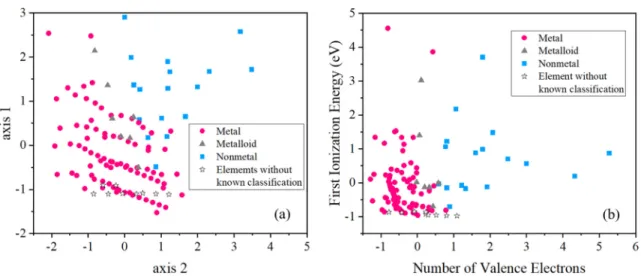
feature importance (the higher the value, the more important the feature) by calculating the normalized total reduction in node impurity caused by each feature [32]. As listed in Table I, the feature importance of all atomic data except for “period” is nonzero, and first ionization energy plays a dominant role in the classification, which is consistent with the fact that first ionization energy is directly related to the feasibility of valence electron transfer, and therefore it is directly relevant to the metallic behavior of elements [3]. On the other hand, the number of valence electrons mainly helps to tackle the irregularities in the region of transition metals. As shown in the second and third level of the decision tree in Fig.2, 11 transition metals are recognized from a mixture of metals, metalloids, and nonmetals. This is because many transition metals contain more than eight valence electrons while metalloids and nonmetals contain less (between 3 and 8). As for the mean atomic radius and atomic number, both of them appear in the bottom nodes of the decision tree with very small feature importance, so they do not play dominant roles in classification. To better understand the data distribution, we perform a principle component analysis (PCA) for the whole data set, and plot the distribution of elements on the reduced plane in Fig.5(a)in the Appendix. For comparison, we also plot the distribution of elements on the plane spanned by first ionization energy and number of valence electrons in Fig.5(b) in the Appendix. Although metals and nonmetals tend to occupy different regions in the reduced plane of the whole data set with five features, the plane spanned by first ionization energy and number of valence electrons exhibits much clearer borders between metals, metalloids, and non-metals, supporting the conclusion from the decision tree that first ionization energy and number of valence electrons are the two most important features.

Because the decision tree is prone to overfit the training data [33] and likely to be biased by the dominant class [29], we further employ the support vector machine (SVM) model, which is effective for small data sets with high-dimensional features [34], and we build three SVM classifiers based on different kernel functions [linear kernel (LK), quadratic kernel (QK), and cubic kernel (CK)] in which the degree of the polynomial kernel controls the flexibility of the SVM [35]. To explore the contribution of each feature in the SVM classifiers, different feature sets are used to train the classifiers and the corresponding training set accuracy is shown in TableIIIin the Appendix. One can see that the four features with nonzero importance are informative enough for accurate classification in the SVM, and the first ionization energy and the number of valence electrons are again crucial for classification, as the classification accuracy would be seriously lowered without them.

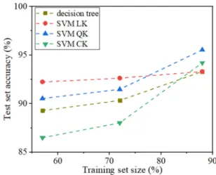
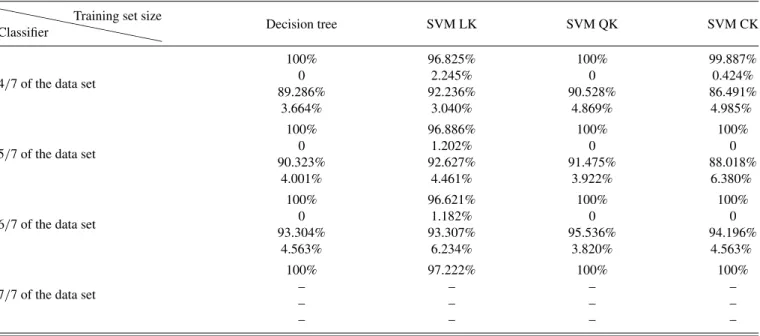
To examine the generalizability, we further split the data set into training sets and test sets, and plot the learning curves [36] of the four classifiers in Fig. 3. We find that, for all the classifiers, the more data in the training sets, the higher

accuracy in the test sets, and they all have accuracy higher than 85% in test sets, demonstrating their predictive ability. More detailed information on the learning curves is provided in TableIVin the Appendix.

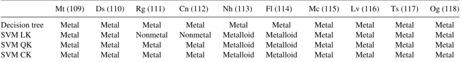
Next, we use the trained classifiers to classify superheavy elements without known classifying labels, and also derive the classification of Cn (Z = 112) for testing the reliability. As shown in Table II, the four classifiers are consistent that Mt, Ds, Mc, Lv, Ts, and Og should be metals. As for Rg, although the SVM LK recognizes this element as a nonmetal, it cannot correctly classify Cn and achieve 100% accuracy in the training set, suggesting that the classification by the SVM LK is not as reliable as other classifiers. Actually, Rg should also be a metal, while both Nh and Fl should be classified as metalloids because the SVM QK and SVM CK outperform the decision tree for a large training set as shown in learning curves.

Then we briefly discuss the classification of Fl and Og (Z = 114 and 118) in which the complex relativistic effects of superheavy elements are well incorporated in our machine learning scheme. Fl is perhaps the most controversial element as some experiments classify it a metal [13,14], while others consider it as a noble gas [9,12]. The origin of such contro-versy is as follows: although Fl has an “open-shell” valence electron configuration of 7s27p2, the 7p orbitals further split into 7p1/2 and 7p3/2 orbitals due to the strong spin-orbital coupling effect [37]. Therefore, the valence electrons of Fl become 7s2_7p

1/22, which form a “closed-shell” configuration

[9]. When describing the volatility of valence electrons, first ionization energy can be used for discussions as shown in Fig. 4(a), where we plot the first ionization energies of Fl and other elements with four valence electrons, showing that the first ionization energy of Fl is slightly higher than that of Si and Ge, but much lower than that of C, supporting our conclusion from machine learning that Fl should be a

FIG. 3. Learning curves of the four classifiers trained using the four features with nonzero importance.

SHENG GONG et al. PHYSICAL REVIEW A 99, 022110 (2019) TABLE II. Classification of Cn and other superheavy elements. For classifying Cn, classifiers are trained for elements with Z= 1 − −108, and for other superheavy elements Cn is added to the training set (Z = 1 − −108, 112). Numbers in parentheses are the atomic numbers.

Mt (109) Ds (110) Rg (111) Cn (112) Nh (113) Fl (114) Mc (115) Lv (116) Ts (117) Og (118) Decision tree Metal Metal Metal Metal Metal Metal Metal Metal Metal Metal SVM LK Metal Metal Nonmetal Nonmetal Metalloid Metalloid Metal Metal Metal Metal SVM QK Metal Metal Metal Metal Metalloid Metalloid Metal Metal Metal Metal SVM CK Metal Metal Metal Metal Metalloid Metalloid Metal Metal Metal Metal

metalloid. As for Og, although it has a closed-shell valence electron configuration of 7s27p6, its p orbitals also split into 7p1/2and 7p3/2, and the electrons in 7p3/2are in high-energy

states and easy to lose. Figure 4(b)shows that the first ion-ization energy of Og is much lower than that of its noble-gas homologs, and close to that of some transition metals, there-fore it is classified as a metal. This is extremely interesting because Og is located in group 18, which is supposed to have similar physical and chemical properties to the other members in the group, most likely resembling Rn, which is above it in the periodic table. However, Og has an anomalously low ion-ization energy, similar to that of lead, which is 70% of radon [38]. In addition, it has been proposed that diatomic molecule Og2would show a bonding interaction approximately equal to

that of Hg2, which is nearly four times as large as that of Rn2

[17]. These features of Og challenge our conventional belief that all elements are organized according to the similarity of their properties in the periodic table, namely, that elements in the same group share similar properties and therefore one can know the characteristics of an element by simply looking at its position in the table.

III. CONCLUSION

In summary, we use four different machine learning clas-sifiers (decision tree, SVM LK, SVM QK, and SVM CK) to explore the relationship between atomic properties and classi-fication of elements. Our analyses show that these classifiers can achieve high accuracy for both training sets and test sets, and the features of first ionization energy and number of valence electrons control the classifications. Furthermore, we

use the classifiers to predict the classifications of superheavy elements, and find that Mt, Ds, Mc, Rg, Lv, Ts, and Og are metals, while Nh and Fl are metalloids. We hope that the present paper can not only demonstrate the effectiveness of machine learning in studying superheavy elements but also deepen our understanding of the periodic table, which provides us the most fundamental information for physics, chemistry, and materials science.

ACKNOWLEDGMENTS

This work is partially supported by grants from the Na-tional Natural Science Foundation of China (NSFC Grant No. 21773004), the National Key Research and Development Program of the Ministry of Science and Technology of China (Grants No. 2016YFE0127300 and No. 2017YFA0204902), and the National Training Program of Innovation for Un-dergraduates of China (Grant No. 201611001008) and is supported by the High Performance Computing Platform of Peking University, China. The authors declare no competing financial interests.

APPENDIX: METHODS 1. Features and data selection

In this paper, five atomic parameters are selected as fea-tures, including atomic number, period, number of valence electrons, first ionization energy, and mean atomic radius. For atomic number, we use the data from IUPAC [39], and for period we assign an integer from 1 to 7 to each element

FIG. 4. First ionization energy of the elements with (a) four and (b) eight valence electrons, respectively. Background coding: bar with vertical lines, metal; bar with tilt lines, metalloids; bar with horizontal lines, nonmetal; bar in blank, elements with unknown classification.

FIG. 5. Distribution of elements on (a) the reduced plane from the five features by PCA and (b) the plane spanned by the first ionization energy and number of valence electrons. Here all features are normalized.

according to the periodic table. The number of electrons in the outermost atomic shell is considered for all elements, while the electrons in the outermost d or f subshell are also considered for transition metals, lanthanides, and actinides, respectively. First ionization energy is included in the data set as it is directly related to metallic behavior. We use the calculated values of first ionization energy reported by Fricke and McMinn [40] for superheavy elements, and the experimental values from the CRC Handbook of Chemistry

and Physics [41] for the others. Such selection is reasonable because different RQM methods give similar values of the first ionization energy [17,21,40], which are close to experimental values [17,21], while for electron affinity different values are obtained by using different RQM methods [21]. Therefore, for data reliability, electron affinity and related electronegativity are not selected as features. The feature of mean atomic radius is considered as it is important in atom drift experiments for superheavy elements [42], and the data including all relativis-tic effects for all elements in the work by Guerra et al. [43] are used.

2. Machine learning classifiers and training sets construction

We use the decision tree classifiers [29] and support vector machine classifiers [30] as implemented in version 0.19.1 of the Scikit-learn package [44]. For the setting of classes, the easiest way to classify elements by properties is to only distinguish them as metals or nonmetals. However, such a scheme is not informative for the elements near the border. For example, Si and Ge have very similar properties, but they are classified into two categories, while Si and H are in the same category (nonmetal) with very different properties. To make the classification more meaningful, we include the class of metalloids in our approach, which contains the elements sharing properties with typical metals and typical nonmetals. Although the set of members in metalloids is in controversy [1,4], the set used in this paper is widely recognized. When using an alternative set with three more elements (C, Se, Po), as shown in Table V in the Appendix, we can still get the same classification for the superheavy elements as the original

set, implying that increasing the size of metalloids would not give us new information, and the original set of metalloids can capture features of metalloids. This is reasonable because the SVM model with a quadratic kernel has very low complexity and can extract information from very small data sets [34]. Actually, if we only include the classes of metals and non-metals, as shown inTable V, the superheavy elements studied here, except for Nh and Fl, would still be classified as metals, while Nh and Fl would be nonmetals. Obviously, the inclusion of metalloids can better describe the properties of Nh and Fl, making the classification more meaningful.

Because there are only seven metalloids in the whole data set, stratified sampling is required for randomly building training sets, otherwise there might not be any metalloid in training sets, which deviates from reality and would largely decrease prediction accuracy. We build four types of training sets, which contain all (7/7), 6/7, 5/7, and 4/7 of the features and classifications of elements, and correspondingly we get three types of test sets with 1/7, 2/7, and 3/7 of elements with known classification (when all elements are included in training sets, there are no data left for test sets). In addition,

FIG. 6. Cross-validation accuracy vs penalty parameter (C) of the three SVM classifiers.

SHENG GONG et al. PHYSICAL REVIEW A 99, 022110 (2019)

TABLE III. Training set accuracy of SVM classifiers trained by different feature sets with all elements with known classification. N, atomic number; P, period; V, number of valence electrons; I, first ionization energy; R, mean atomic radius.

XXXXX_XXXX

Classifier

Feature set

NPVIR NVIR VIR NIR NVR NVI

SVM LK 97% 97% 94% 87% 63% 97%

SVM QK 100% 100% 100% 86% 62% 100%

SVM CK 100% 100% 100% 87% 71% 93%

TABLE IV. Detailed information on the learning curves of the four classifiers trained by training sets with different sizes. Values in the vertical sequence are training set accuracy, standard deviation of training set accuracy, test set accuracy, and standard deviation of test set accuracy, respectively.

``````_`````

Classifier

Training set size

Decision tree SVM LK SVM QK SVM CK

4/7 of the data set

100% 96.825% 100% 99.887%

0 2.245% 0 0.424%

89.286% 92.236% 90.528% 86.491%

3.664% 3.040% 4.869% 4.985%

5/7 of the data set

100% 96.886% 100% 100%

0 1.202% 0 0

90.323% 92.627% 91.475% 88.018%

4.001% 4.461% 3.922% 6.380%

6/7 of the data set

100% 96.621% 100% 100%

0 1.182% 0 0

93.304% 93.307% 95.536% 94.196%

4.563% 6.234% 3.820% 4.563%

7/7 of the data set

100% 97.222% 100% 100%

– – – –

– – – –

– – – –

TABLE V. Classification of superheavy elements with different classes by SVM QK.

Mt Ds Rg Cn Nh Fl Mc Lv Ts Og

(109) (110) (111) (112) (113) (114) (115) (116) (117) (118) Set used in this paper Metal Metal Metal Metal Metalloid Metalloid Metal Metal Metal Metal Set with three more metalloids (C, Se, Po) Metal Metal Metal Metal Metalloid Metalloid Metal Metal Metal Metal Set with only metals and nonmetals Metal Metal Metal Metal Nonmetal Nonmetal Metal Metal Metal Metal

cross-validation procedures [44] are carried out for the penalty parameter (C) of the three SVM classifiers with the training sets of 5/7 for all elements with known classification, and the results are given in Fig.6 in the Appendix, from which we can pick up the most robust C value (with the maximum accuracy). We further verify the reliability of the picked models by plotting learning curves, as shown in Fig.3. Since

the accuracy of a single test is influenced by the random partition of the data set, when doing cross validation we repeat the test five times with different training sets to get the average accuracy of the model, and increase the number of repetitions to 10 when plotting the learning curves.

Figures5and6and TablesIII–Vin this Appendix provide further details related to the discussion in the main text.

[1] R. E. Vernon,J. Chem. Educ. 90,1703(2013).

[2] P. P. Edwards and M. J. Sienko,Accounts Chem. Res. 15,87

(2002).

[3] M. R. Leach,Found. Chem. 15,13(2012).

[4] R. H. Goldsmith,Metalloids. J. Chem. Educ. 59,526(1982). [5] R. Smolanczuk,Phys. Rev. C 59,2634(1999).

[6] P. P. Edwards and M. J. Sienko,J. Chem. Educ. 60,691(1983). [7] S. J. Hawkes,J. Chem. Educ. 78,1686(2001).

[8] S. Hofmann,Nat. Chem. 2,146(2010).

[9] C. E. Düllmann,Radiochim. Acta 100,67(2012).

[10] N. V. Aksenov, P. Steinegger, F. S. Abdullin, Y. V. Albin, G. A. Bozhikov, V. I. Chepigin, R. Eichler, V. Y. Lebedev, A. S. Madumarov, O. N. Malyshev et al., Eur. Phys. J. A 53,158

(2017).

[11] R. Eichler,J. Phys. Conf. Ser. 420,012003(2013).

[12] D. Rudolph, A. Yakushev, and R. Eichler,EPJ Web Conf.131,

07003(2016).

[13] R. Eichler et al.,Radiochim. Acta 98,133(2010). [14] A. Yakushev et al.,Inorg. Chem. 53,1624(2014). [15] J. Styszy´nski,J. Phys. Conf. Ser. 104,012025(2008). [16] I. P. Grant,Aust. J. Phys. 39,649(1986).

[17] C. S. Nash,J. Phys. Chem. A 109,3493(2005).

[18] P. Schwerdtfeger, L. F. Pašteka, A. Punnett, and P. O. Bowman,

Nucl. Phys. A 944,551(2015).

[19] W. Kutzelnigg,Chem. Phys. 395,16(2012).

[20] K. Liu, C. G. Ning, and J. K. Deng,Phys. Rev. A 80,022716

(2009).

[21] A. Borschevsky, L. F. Pašteka, V. Pershina, E. Eliav, and U. Kaldor,Phys. Rev. A 91,020501(2015).

[22] P. Indelicato, J. P. Santos, S. Boucard, and J. P. Desclaux,Eur. Phys. J. D 45,155(2007).

[23] L. B. Richard,J. Chem. Educ. 39,251(1962). [24] L. C. Allen,J. Am. Chem. Soc. 111,9003(1989). [25] M. I. Jordan and T. M. Mitchell,Science 349,255(2015). [26] J. P. Janet and H. J. Kulik,Chem. Sci. 8,5137(2017). [27] Q Zhou, P. Tang, S. Liu, J. Pan, Q. Yan, and S. Zhang,Proc.

Natl. Acad. Sci. USA 115,E6411(2018).

[28] P Raccuglia et al.,Nature (London) 533,73(2016).

[29] H. Blockeel and J. Struyf, J. Mach. Learn. Res. 3, 621 (2003). [30] C. Cortes and V. Vapnik,Mach. Learn. 20,273(1995). [31] F. Xia, W. Zhang, F. Li, and Y. Yang,Knowl. Inf. Syst. 17,381

(2008).

[32] J. Praagman,Eur. J. Oper. Res. 19,144(1985).

[33] C. W. Tung et al.,Scientific World J.2013,782031(2013). [34] D.-C. Li and C.-W. Liu,Expert Syst. Appl. 37,3104(2010). [35] B. K. Yeo and Y. Lu,IET Microw. Antenna. P. 6,1473(2012). [36] I. Venezia,Eur. J. Oper. Res. 19,191(1985).

[37] P. Pyykko and J. P. Desclaux,Accounts Chem. Res. 12, 276

(1979).

[38] Y. K. Han, C. Bae, S. K. Son, and Y. S. Lee,J. Chem. Phys. 112,

2684(2000).

[39] M. E. Wieser and M. Berglund,Pure Appl. Chem. 81, 2131

(2009).

[40] B. Fricke and J. McMinn,Naturwissenschaften 63,162(1976). [41] GLE Turner,Ann. Sci. 48,313(1991).

[42] M. Sewtz, M. Laatiaoui, K. Schmid, and D. Habs,Eur. Phys. J. D 45,139(2007).

[43] M. Guerra, P. Amaro, J. P. Santos, and P. Indelicato,Atom. Data Nucl. Data 117-118,439(2017).

[44] F Pedregosa, G. Varoquaux, A. Gramfort, V. Michel, B. Thirion, O. Grisel, M. Blondel, P. Prettenhofer, R. Weiss, V. Dubourg et al., J. Mach. Learn. Res. 12, 2825 (2011).