HAL Id: hal-00431265
https://hal.archives-ouvertes.fr/hal-00431265
Preprint submitted on 11 Nov 2009HAL is a multi-disciplinary open access
archive for the deposit and dissemination of sci-entific research documents, whether they are pub-lished or not. The documents may come from teaching and research institutions in France or
L’archive ouverte pluridisciplinaire HAL, est destinée au dépôt et à la diffusion de documents scientifiques de niveau recherche, publiés ou non, émanant des établissements d’enseignement et de recherche français ou étrangers, des laboratoires
TVaR-based capital allocation with copulas
Mathieu Bargès, Hélène Cossette, Etienne Marceau
To cite this version:
Mathieu Bargès, Hélène Cossette, Etienne Marceau. TVaR-based capital allocation with copulas. 2009. �hal-00431265�
TVaR-based capital allocation with copulas
Mathieu Barg`es∗‡ H´el`ene Cossette‡ Etienne Marceau´ ‡
Abstract
Because of regulation projects from control organizations such as the European solvency II reform and recent economic events, insurance companies need to consolidate their capital reserve with coherent amounts allocated to the whole company and to each line of business. The present study considers an insurance portfolio consisting of several lines of risk which are linked by a copula and aims to evaluate not only the capital allocation for the overall portfolio but also the contribution of each risk over their aggregation. We use the tail value at risk (TVaR) as risk measure. The handy form of the FGM copula permits an exact expression for the TVaR of the sum of the risks and for the TVaR-based allocations when claim amounts are exponentially distributed and distributed as a mixture of exponentials. We first examine the bivariate model and then the multivariate case. We also show how to approximate the TVaR of the aggregate risk and the contribution of each risk when using any copula.
Keywords: Capital allocation; Tail value at risk; Dependence models; Copulas; Discretization
methods
1
Introduction
In recent years, a lot of research has focused on insurance capital allocation. Indeed the European Solvency II project and the recent events encourage insurance companies to consolidate their finan-cial reserves and investments. Risk measures are well-known tools to determine the capital amount that has to be allocated to a risk portfolio. Artzner et al. (1999) proposed an axiomal definition of a coherent risk measure that can be used for allocation issues. This coherence property has also been discussed inWang(2002). Using their definition,Artzner et al.(1999) proposed the tail value at risk (TVaR), also called expected shortfall (ES), as a coherent alternative to the non-coherent risk measure value at risk (VaR). Applied to continuous random variables, the TVaR can identi-cally be defined as the conditional tail expectation (CTE). But these two risk measures differ in discrete contexts where the CTE is no longer coherent. The differences between these definitions and properties have been highlighted in Acerbi et al.(2001) andAcerbi and Tasche (2002).
In the literature on capital allocation, continuous situations are widely studied in contrast with discrete cases. That is why most of the references speak in terms of CTE. The capital
allocation principle has first been introduced by Tasche (1999) where the capital allocated to each risk is expressed in terms of the CTE of the aggregate risk. This top down allocation me-thod has then been used to provide several closed formulae and approximations of the CTE and the CTE-based allocations for different types of multivariate continuous distributions. The first multivariate top down model was considered by Panjer (2002) where the risks have a multiva-riate normal distribution. This work has been extended to a multivamultiva-riate elliptical distribution in
Landsman and Valdez(2003) and inDhaene et al. (2008). A multivariate gamma distribution for risks has been studied in Furman and Landsman (2005) as well as a multivariate Tweedie distri-bution in Furman and Landsman (2007). In these papers, explicit expressions for the CTE and the CTE-based allocation are derived. Other closed form expressions for the CTE of the sum of multivariate phase-type distributed risks and the contribution of one risk to the portfolio have been given in Cai and Li (2005). More recently, Chiragiev and Landsman (2007) found a CTE and CTE-based allocation for multivariate Pareto risks. Further information on the CTE-based allocation of risk capital can be found inKim (2007).
In most papers mentioned above, the dependence between the different lines of business of the insurance company is due to the construction of a multivariate distribution. In the present paper, we propose introducing dependence with a copula. Copulas are currently seen as effective and flexible tools to represent dependence between random variables. Furthermore, in order to have the risk measure coherence property in every continuous and discrete situation, we propose using the TVaR as defined in Acerbi et al.(2001) and Acerbi and Tasche (2002) to develop a top down approach of the capital allocation. Indeed, the Committee of European Insurance and Occupational Pensions Supervisors (CEIOPS) advises in the Solvency II context the use of the TVaR for the evaluation of the Solvency Capital Requirement (SCR); seeCEIOPS (2006) andCEIOPS (2007).
First, closed form expressions for the TVaR and then the TVaR-based contribution of one risk over the aggregation of all risks are obtained when the Farlie-Gumbel-Morgenstern copula describes the dependence between the risk marginals. With most copulas introducing dependence between different risks however, we are not able to reach closed form expressions. Consequently, we also present approximation methods to evaluate the TVaR and the TVaR-based allocation by the use of different discretization methods of continuous random variables which are applicable with any copula and any marginals.
In the first section, we give the general definitions for the tail value at risk of the aggregate risk and the contribution of one of the risks. The second section deals with the application of the TVaR-based allocation rule using the FGM copula and exponential distributed risks. We first consider two lines of business and then pursue to a multivariate context. We widen our results to risks that are distributed as mixture of exponentials in section 3. For these two last sections, we are able to have closed form expressions for both the TVaR and the individual risk contribution based on it. Then, we expose approximation methods for the TVaR and TVaR-based allocation when the dependence structure is defined by any copula. The results are illustrated with numerical applications.
2
Definition of the TVaR and the TVaR-based allocation
In this section, we define the tail value at risk (TVaR) for the aggregate risk and the TVaR-based allocation rule. We consider the aggregate claim amount (or loss) S of a portfolio of n risks. The claim amount (or loss) for risk i is denoted by Xi. Thus we have S = X1+ ... + Xnwhere all Xi’s are non-negative random variables.
The value at risk at level κ, 0 < κ < 1, of S is defined by
V aRκ(S) = inf (x∈ R, FS(x)≥ κ).
It is well known that the VaR is a risk measure that is not coherent. Thus we choose to work with the tail value at risk of S as introduced in Acerbi and Tasche (2002), Schmock and Straumann
(1999) and Schmock(2006) at level κ, for κ∈ (0, 1). Its definition is
T V aRκ(S) = 1 1− κ ∫ 1 κ V aRu(S)du = E[S1{S>V aRκ(S)} ] + V aRκ(S) ( P r (S≤ V aRκ(S))− κ ) 1− κ ,
which is a coherent risk measure. When S is continuous, P r(S ≤ V aRκ(S)) = κ which implies that the TVaR is exactly the conditional tail expectation (CTE) meaning T V aRκ(S) = E[S|S >
V aRκ(S)] = CT E(S). In financial risk management, the TVaR is called the expected shortfall. The additivity of the expectation allows the decomposition of the TVaR (CTE) into the sum of TVaR contributions as follows
T V aRκ(S) = n ∑
i=1
T V aRκ(Xi; S),
where the TVaR contribution of the ith risk to the total risk represents the part of the capital that is allocated to risk i. For κ∈ (0, 1), it can be expressed as
T V aRκ(Xi; S) = E [ Xi× 1{S>V aRκ(S)} ] + βSE[Xi× 1{S=V aRκ(S)} ] 1− κ , with βS= {P r(S≤V aR κ(S))−κ P r(S=V aRκ(S)) , if P r (S = V aRκ(S)) > 0, 0, otherwise.
For continuous distributions, we have T V aRκ(Xi; S) = 1 1− κE [ Xi× 1{S>V aRκ(S)} ] = E[Xi | S > V aRκ(S)] = CT Eκ(Xi|S).
That means that the TVaR-based contribution of one risk is equal to the CTE-based contribution of the same risk when all the marginals are continuous.
Note that E[Xi | S = s] = E[Xi| X1+ ... + Xn= s] = ∫ s 0 xfXi|S(x| S = s)dx = ∫ s 0 xfXi,S(x, s) fS(s) dx. Then, the CTE-based contribution can be expressed as
CT Eκ(Xi|S) = ∫ ∞ V aRκ(S) E[Xi | S = s]fS|S>V aRκ(S)(s)ds = 1 P r(S > V aRκ(S)) ∫ ∞ V aRκ(S) E[Xi| S = s]fS(s)ds = 1 1− κ ∫ ∞ V aRκ(S) ∫ s 0 xfXi,S(x, s)dxds. (1)
3
TVaR and the TVaR-based allocation with exponential
margi-nals and the FGM copula
In this section, we derive the expression for the TVaR and the TVaR-based allocation for two exponentially distributed risks joined by a FGM copula. We also extend the results obtained with this bivariate model to a multivariate model. The exponential distribution is a classical distribution for the risk random variables. Its convenient and practical mathematic properties permit to develop explicit results. We are aware that the FGM copula introduces only light dependence. However, it admits positive as well as negative dependence between a set of random variables. As said in
Yeo and Valdez(2006) where the FGM copula is used to link claim variables in a credibility model, even if it can model only weak dependence, the FGM copula permits to assign a unique dependence parameter for each pair or group of risks and allows a more complex dependence structure than most of the copulas which use only one or few parameters. Furthermore, its handy form allows explicit calculus and thus exact results. This copula was also used to describe different correlation relations on the financial markets in Gatfaoui (2005) and Gatfaoui (2007).
3.1 The bivariate case
Let X1and X2be two exponentially distributed random variables representing the claim amounts of two insurance risks. Their cumulative distribution functions (cdf) and probability density functions (pdf) are given by
FXi(xi) = 1− e−λ ixi,
fXi(xi) = λie
−λixi, for i = 1, 2.
In order to simplify our presentation, we restrain our study to the constraints λ1 ̸= λ2, λ1 ̸= 2λ2, λ2 ̸= 2λ1. It is possible to find adjusted results without these constraints by applying a similar method as the one exposed below.
A dependence structure for (X1, X2) based on the bivariate FGM copula is introduced. The FGM copula is defined by
CθF GM(u1, u2) = u1u2+ θu1u2(1− u1)(1− u2) for ui∈ [0, 1], i = 1, 2, and dependence parameter θ ∈ [−1, 1].
The density of the bivariate FGM copula is
cF GMθ (u1, u2) = ∂2CθF GM(u1, u2) ∂u1∂u2 = 1 + θ(1− 2u1)(1− 2u2) = 1 + θ(2u1− 1)(2u2− 1), where ui = 1− ui, i = 1, 2.
The TVaR of the aggregate risk S = X1+ X2 is given in the following proposition.
Proposition 1 Let X1 and X2 be two exponentially distributed random variables with joint cdf defined by a bivariate FGM copula as follows
FX1,X2(x1, x2) = C
F GM
θ (FX1(x1), FX2(x2)),
with θ ∈ [−1, 1]. Then, the TVaR of the aggregate risk S = X1+ X2 at level κ, 0 < κ < 1, is T V aRκ(S) = 1 1− κ [ (1 + θ)ζ(V aRκ(S); λ1; λ2)− θζ(V aRκ(S); 2λ1; λ2) −θζ(V aRκ(S); λ1; 2λ2) + θζ(V aRκ(S); 2λ1; 2λ2) ] , (2) where ζ(x; γ1, γ2) = γ2γ−γ2 1e−γ1x ( x +γ1 1 ) + γ1 γ1−γ2e −γ2x ( x +γ1 2 ) .
Proof. The joint pdf of (X1, X2) is given by fX1,X2(x1, x2) = c F GM θ (FX1(x1), FX2(x2))fX1(x1)fX2(x2) = fX1(x1)fX2(x2) + θfX1(x1)fX2(x2)(1− 2FX1(x1))(1− 2FX2(x2)) = (1 + θ)λ1e−λ1x1λ2e−λ2x2 − θ2λ1e−2λ1x1λ2e−λ2x2 −θλ1e−λ1x12λ2e−2λ2x2 + θ2λ1e−2λ1x12λ2e−2λ2x2.
Let h(x, λ1, λ2) be the distribution function of a generalized Erlang random variable X h(x, λ1, λ2) = λ1λ2 λ2− λ1 e−λ1x+ λ1λ2 λ1− λ2 e−λ2x.
Then, the pdf of S can be expressed as a combination of generalized Erlang pdf’s
fS(s) = ∫ s 0 fX1,S(x, s)dx = ∫ s 0 fX1,X2(x, s− x)dx = (1 + θ)h(s; λ1; λ2)− θh(s; 2λ1; λ2)− θh(s; λ1; 2λ2) + θh(s; 2λ1; 2λ2), (3) where the first component of fS(s) is
∫ s 0 (1 + θ)λ1e−λ1xλ2e−λ2(s−x)dx = (1 + θ)λ1λ2e−λ2s ∫ s 0 ex(λ2−λ1)dx = (1 + θ) λ1λ2 λ2− λ1 e−λ1s+ (1 + θ) λ1λ2 λ1− λ2 e−λ2s = (1 + θ)h(s; λ1; λ2). The three other components can be found similarly.
Thus, the TVaR of S takes the form
T V aRκ(S) = E[S| S > V aRκ(S)] = ∫ ∞ V aRκ s fS(s) P r(S > V aRκ(S)) ds = 1 1− FS(V aRκ(S)) ∫ ∞ V aRκ(S) sfS(s)ds = 1 1− κ ∫ ∞ V aRκ(S) s [ (1 + θ)h(s; λ1; λ2)− θh(s; 2λ1; λ2) −θh(s; λ1; 2λ2) + θh(s; 2λ1; 2λ2) ] ds. (4)
Define ∫ ∞ V aRκ(S) sh(s; λ1; λ2)ds = ∫ ∞ V aRκ(S) s ( λ1λ2 λ2− λ1 e−λ1s+ λ1λ2 λ1− λ2 e−λ2s ) ds = λ1λ2 λ2− λ1 {[ −se−λ1s λ1 ]∞ V aRκ(S) + ∫ ∞ V aRκ(S) e−λ1s λ1 ds } + λ1λ2 λ1− λ2 {[ −se−λ2s λ2 ]∞ V aRκ(S) + ∫ ∞ V aRκ(S) e−λ2s λ2 ds } = λ1λ2 λ2− λ1 ( V aRκ(S)e −λ1V aRκ(S) λ1 +e −λ1V aRκ(S) λ2 1 ) + λ1λ2 λ1− λ2 ( V aRκ(S)e −λ2V aRκ(S) λ2 +e −λ2V aRκ(S) λ2 2 ) = λ2 λ2− λ1 e−λ1V aRκ(S) ( V aRκ(S) + 1 λ1 ) + λ1 λ1− λ2 e−λ2V aRκ(S) ( V aRκ(S) + 1 λ2 ) = ζ(V aRκ(S); λ1, λ2). (5) Inserting (5) in (4), we obtain T V aRκ(S) = 1 1− κ [ (1 + θ)ζ(V aRκ(S); λ1; λ2)− θζ(V aRκ(S); 2λ1; λ2) −θζ(V aRκ(S); λ1; 2λ2) + θζ(V aRκ(S); 2λ1; 2λ2) ] , with ζ(x; γ1, γ2) = γ2 γ2− γ1 e−γ1x ( x + 1 γ1 ) + γ1 γ1− γ2 e−γ2x ( x + 1 γ2 ) .
A closed form expression for the TVaR-based capital attributed to risk i, i = 1, 2, is given in the next proposition.
Proposition 2 Let X1 and X2 be two exponentially distributed random variables with joint cdf defined by a bivariate FGM copula. Then, the TVaR-based contribution of risk i, i = 1, 2, to the aggregate risk S = X1+ X2 at level κ, 0 < κ < 1, is
T V aRκ(Xi; S) = 1 1− κ
[
(1 + θ)ξ (V aRκ(S); λi; λj)− θξ (V aRκ(S); 2λi; λj)
−θξ (V aRκ(S); λi; 2λj) + θξ (V aRκ(S); 2λi; 2λj) ]
where ξ (x; γi; γj) =
γje−γix(x+γi1)
γj−γi −
γje−γix−γie−γjx
(γj−γi)2 and i̸= j.
Proof. Let i = 1 and j = 2. Recall that for continuous random variables the TVaR-based allocation is equal to the CTE-based allocation. From (1), we have
T V aRκ(X1; S) = E[X1| S > V aRκ(S)] = 1 P r(S > V aRκ(S)) ∫ ∞ V aRκ(S) ∫ s 0 xfX1,S(x, s)dxds, where ∫ s 0 xfX1,S(x, s)dx = ∫ s 0 xfX1,X2(x, s− x)dx = ∫ s 0 x ( (1 + θ)λ1e−λ1xλ2e−λ2(s−x)− θ2λ1e−λ1xλ2e−λ2(s−x) −θλ1e−λ1x2λ2e−λ2(s−x)+ θ2λ1e−λ1x2λ2e−λ2(s−x) ) dx = (1 + θ)λ1λ2 ( se−λ1s λ2− λ1 − e−λ1s− e−λ2s (λ2− λ1)2 ) −θ2λ1λ2 ( se−2λ1s λ2− 2λ1 − e−2λ1s− e−λ2s (λ2− 2λ1)2 ) −θλ12λ2 ( se−λ1s 2λ2− λ1 − e−λ1s− e−2λ2s (2λ2− λ1)2 ) +θ2λ12λ2 ( se−2λ1s 2λ2− 2λ1 − e−2λ1s− e−2λ2s (2λ2− 2λ1)2 ) .
The first component on the right-hand side of the last equality is given by ∫ s 0 x(1 + θ)λ1e−λ1xλ2e−λ2(s−x)dx = (1 + θ)λ1λ2e−λ2s ∫ s 0 xex(λ2−λ1)dx = (1 + θ)λ1λ2e−λ2s ([ xe x(λ2−λ1) λ2− λ1 ]s 0 − ∫ s 0 ex(λ2−λ1) λ2− λ1 dx ) = (1 + θ)λ1λ2e−λ2s ( se s(λ2−λ1) λ2− λ1 − [ ex(λ2−λ1) (λ2− λ1)2 ]s 0 ) = (1 + θ)λ1λ2e−λ2s ( se sλ2e−sλ1 λ2− λ1 − esλ2e−sλ1− 1 (λ2− λ1)2 ) = (1 + θ)λ1λ2 ( se−λ1s λ2− λ1 − e−λ1s− e−λ2s (λ2− λ1)2 ) .
Denoting V = V aRκ(S), we have T V aRκ(X1; S) = 1 1− FS(V ) ∫ ∞ V { (1 + θ)λ1λ2 ( se−λ1s λ2− λ1 − e−λ1s− e−λ2s (λ2− λ1)2 ) −θ2λ1λ2 ( se−2λ1s λ2− 2λ1 − e−2λ1s− e−λ2s (λ2− 2λ1)2 ) − θλ12λ2 ( se−λ1s 2λ2− λ1 − e−λ1s− e−2λ2s (2λ2− λ1)2 ) +θ2λ12λ2 ( se−2λ1s 2λ2− 2λ1 − e−2λ1s− e−2λ2s (2λ2− 2λ1)2 ) } ds = 1 1− FS(V ) [ (1 + θ) ( λ2e−λ1V(V +λ11) λ2− λ1 − λ2e−λ1V − λ1e−λ2V (λ2− λ1)2 ) −θ ( λ2e−2λ1V(V +2λ11) λ2− 2λ1 − λ2e−2λ1V − 2λ1e−λ2V (λ2− 2λ1)2 ) −θ ( 2λ2e−λ1V(V +λ11) 2λ2− λ1 − 2λ2e−λ1V − λ1e−2λ2V (2λ2− λ1)2 ) +θ ( 2λ2e−2λ1V(V + 2λ11) 2λ2− 2λ1 − 2λ2e−2λ1V − 2λ1e−2λ2V (2λ2− 2λ1)2 ) ] . We finally obtain T V aRκ(X1; S) = 1 1− κ [ (1 + θ)ξ (V aRκ(S); λ1; λ2)− θξ (V aRκ(S); 2λ1; λ2) −θξ (V aRκ(S); λ1; 2λ2) + θξ (V aRκ(S); 2λ1; 2λ2) ] , where ξ (x; γ1; γ2) = γ2e−γ1x(x + γ11) γ2− γ1 − γ2e−γ1x− γ1e−γ2x (γ2− γ1)2 .
The TVaR-based allocation for the second risk is symmetrically given by
T V aRκ(X2; S) = 1 1− κ [ (1 + θ)ξ (V aRκ(S); λ2; λ1)− θξ (V aRκ(S); 2λ2; λ1) −θξ (V aRκ(S); λ2; 2λ1) + θξ (V aRκ(S); 2λ2; 2λ1) ] , where ξ (x; γ2; γ1) = γ1e−γ2x(x + γ12) γ1− γ2 − γ1e−γ2x− γ2e−γ1x (γ1− γ2)2 .
Remark 3 It can be verified that the TVaR of S is the sum of the risk contributions T V aRκ(S) = 2 ∑ i=1 T V aRκ(Xi; S).
Explicit expressions for the TVaR and the one risk TVaR-based contribution cannot only be obtained in the bivariate case but even for an undefined number of risks.
3.2 The multivariate case
Suppose now that there are n different exponential risks joined by a multivariate FGM copula characterized by C (u1, u2, ..., un) = u1u2...un 1 +∑n k=2 ∑ 1≤j1<...<jk≤n θj1j2...jkuj1uj2...ujk ,
where u(.) = 1− u(.) (see Nelsen (2006) p.108). We have here 2n− n − 1 copula parameters to describe the dependence between each pair or group of risks.
Its density can be written as
c (u1, u2, ..., un) = 1 + n ∑ k=2 ∑ 1≤j1<...<jk≤n
θj1j2...jk(2uj1 − 1)(2uj2 − 1)...(2ujk − 1).
As in the bivariate case, we suppose that the parameters of the n exponential risks satisfy the conditions below
λi̸= λj and λi̸= 2λj for i̸= j. (7)
Then, the following proposition holds.
Proposition 4 Let Sn= X1+X2+...+Xnbe the sum of n dependent exponential random variables with joint cdf defined by a multivariate FGM copula as follows
FX1,...,Xn(x1, ..., xn) = C
F GM
θ (FX1(x1), ..., FXn(xn))
with θ ∈ [−1, 1]. Then, the TVaR of Sn at level κ, 0 < κ < 1, is
T V aRκ(Sn) = 1 1− κ× [ 1 + n ∑ k=2 ∑ 1≤j1<...<jk≤n θj1j2...jk× ∑k l=0 ∑ (a1,...,ak)∈Al,k (−1)lζ(V aRκ(Sn); 2i1λ1, ..., 2ikλk, λik+1, ...λin )] , (8)
where ζ(x; γ1, ..., γn) = ∑n i=1 (∏n j=1,j̸=i γj γj−γi ) e−γix ( x +γ1 i )
, ik+1, ..., in are the missing indexes
of j1, ..., jkto complete 1, ..., n and Al,k are the sets of k-tuples composed of l zeros and (k− l) ones,
for l = 0, 1, ..., k and k = 2, ..., n.
In fact, the Al,k are defined by A0,k = { (1, 1, ..., 1)1×k}, A1,k = { (1, 1, ..., 0)1×k, ..., (0, 1, ..., 1)1×k}, A2,k = { (1, 1, ..., 0, 0)1×k, ..., (0, 0, ..., 1)1×k}, ... , Ak,k = { (0, 0, ..., 0)1×k}. Proof. The joint pdf of (X1, X2, ..., Xn) is
fX1,X2,...,Xn(x1, x2, ..., xn) = c(FX1(x1), FX2(x2), ..., FXn(xn))fX1(x1)fX2(x2)...fXn(xn) = fX1(x1)fX2(x2)...fXn(xn) ×[1 + n ∑ k=2 ∑ 1≤j1<...<jk≤n θj1j2...jk(1− FXj1(xj1))(1− FXj2(xj2))...(1− FXjk(xjk)) ] .
As the n risk random variables are exponentially distributed with parameters λi, i = 1, ..., n with constraint (7), we have fX1,X2,...,Xn(x1, x2, ..., xn) = λ1e−λ 1x1λ 2e−λ2x2...λne−λnxn ×[1 + n ∑ k=2 ∑ 1≤j1<...<jk≤n θj1j2...jk(2e −λj1xj1 − 1)(2e−λj2xj2 − 1)...(2e−λjnxjn − 1) ] = ν(x1, x2, ..., xn; λ1, λ2, ..., λn) + n ∑ k=2 ∑ 1≤j1<...<jk≤n θj1j2...jk ×[ k ∑ l=0 ∑ (a1,...,ak)∈Al,k (−1)lν(xj1, xj2, ..., xjk, xik+1, ..., xin; 2 a1λ j1, 2 a2λ j2, ..., 2 akλ jk, λik+1, ..., λin) ] , (9)
where ik+1, ..., in and Al,k are defined as in the proposition and
ν(x1, ..., xn; γ1, ..., γn) = γ1e−γ1x1 × γ2e−γ2x2 × ... × γne−γnxn. Given that fSn(s) = ∫ s 0 ∫ s−x1 0 ... ∫ s−x1−...−xn−1 0 fX1,X2,...,Xn−1,Xn(x1, x2, ..., xn−1, s− x1− x2− ... − xn−1)dx1dx2...dxn−1 = ∫ s 0 ∫ s−x1 0 ... ∫ s−x1−...−xn−2 0 fX1,X2,...,Xn−2,Xn−1+Xn(x1, x2, ..., xn−2, s− x1− x2− ... − xn−2)dx1dx2...dxn−2 = ... = ∫ s 0 fX1,X2+...+Xn(x1, s− x1)dx1
and that ∫ s 0 ∫ s−x1 0 ... ∫ s−x1−...−xn−1 0 ν(x1, x2, ..., xn; γ1, γ2, ..., γn)dx1dx2...dxn−1= n ∑ i=1 ∏n j=1,j̸=i γj γj− γi γie−γis = h(s; γ1, γ2, ...γn), one can write
fSn(s) = h (s; λ1, ..., λn) + n ∑ k=2 ∑ 1≤j1<...<jk≤n θj1j2...jk ∑k l=0 ∑ (a1,...,ak)∈Al,k (−1)lh(s; 2a1λ j1, 2 a2λ j2, ..., 2 akλ jk, λik+1, ...λin ) .
Then, the TVaR of Sn for n≥ 2 and 0 < κ < 1 is
T V aRκ(Sn) = E[Sn| Sn> V aRκ(Sn)] = ∫ ∞ V aRκ s fSn(s) P r(Sn> V aRκ(Sn)) ds = 1 1− κ ∫ ∞ V aRκ(Sn) sfSn(s)ds = 1 1− κ× [ 1 + n ∑ k=2 ∑ 1≤j1<...<jk≤n θj1j2...jk× ∑k l=0 ∑ (a1,...,ak)∈Al,k (−1)lζ(V aRκ(Sn); 2i1λ1, ..., 2ikλk, λik+1, ...λin )] , where ζ(x; γ1, ..., γn) = n ∑ i=1 ∏n j=1,j̸=i γj γj− γi e−γix ( x + 1 γi ) .
As in the bivariate case, the capital allocation for risk i can also be explicitly given. In order to find that expression, we first need to introduce the nth order divided difference of a function f as inChiragiev and Landsman(2007). Consider x1, x2, ..., xn, xn+1 arbitrary points such that xi ̸= xj for i̸= j. The nth order divided difference of f on x1, x2, ..., xn, xn+1 is defined by
f (x1, x2, ..., xn, xn+1) = n+1 ∑ i=1 f (xi) ∏ j̸=i(xi− xj) .
Proposition 5 Let X1, ..., Xnbe n exponentially distributed random variables with joint cdf defined
by a multivariate FGM copula. Then, the TVaR-based contribution of risk i, i = 1, ..., n, to the sum Sn= X1+ ... + Xn at level κ, 0 < κ < 1, is T V aRκ(Xi; Sn) = (−1) n−1Λ 1− κ [ Hi(V aRκ(Sn); λ1; ...; λn) + n ∑ k=2 ∑ 1≤j1<...<jk≤n∩i∈{j1,...,jk} θj1...jk× (k−1 ∑ l=0 ∑ (a1,...,ak)−i∈Al,k−1
{ (−1)l+12k−1−lHi(V aRκ(Sn); 2a1λ j1; ...; 2 akλ jk; λik+1; ...λin) +(−1)l2k−1−lGi(V aRκ(Sn); 2a1λj1; ...; 2 akλ jk; λik+1; ...λin) }) + n−1 ∑ k=2 ∑ 1≤j1<...<jk≤n ∩ i /∈{j1,...,jk} θj1...jk× ( k ∑ l=0 ∑ (a1,...,ak)∈Al,k (−1)l2k−lHi(V aRκ(Sn); 2a1λj1; ...; 2 akλ jk; λik+1; ...λin) )] , (10)
where Hi(x; γ1, ..., γi−1, γi+1, ..., γn) and Gi(x; γ1, ..., γi−1, γi+1, ..., γn) are the (n− 2)-th order
di-vided differences of respectively Hi(x; γ) = γxe−γix
i(γi−γ) + e−γix γ2 i(γi−γ) + γe−γix−γie−γx γγi(γi−γ)2 and Gi(x; γ) = 2 ( xe−2γix 2γi(2γi−γ)+ e−2γix (2γi)2(2γi−γ)+ γe−2γix−2γie−γx γ2γi(2γi−γ)2 )
, Λ = λ1 × ... × λn is the product of the parameters
of exponential distributions, ik+1, ..., in are the missing indexes of j1, ..., jk to complete 1, ..., n and
Al,k are the sets of k-tuples composed of l zeros and (k− l) ones, for l = 0, 1, ..., k and k = 2, ..., n.
Proof. The capital attributed to the continuous distributed risk i can be expressed as T V aRκ(Xi; Sn) = CT Eκ(Xi|Sn) = 1 FSn(V aRκ(Sn)) ∫ ∞ V aRκ(Sn) ∫ s 0 xifXi,Sn(xi, s)dxds. (11)
A recursive formula for fXi,Sn(xi, s) = fXi,Sn−Xi(xi, s− xi) is needed to evaluate this
expres-sion. Given that the risk random variables here are not independent, we cannot directly separate
fXi,Sn−Xi(xi, s− xi) into the product of fXi(xi) and fSn−1(s− xi). First, we have fXi,Sn−Xi(xi, s− xi) = fXi,X1+X2+...+Xi−1+Xi+1+...+Xn(xi, s− xi) = ∫ s−xi 0 ∫ s−xi−x1 0 ∫ s−xi−x1−x2 0 ... ∫ s−x1−...−xn−1 0 fX1,X2,...,Xn−1,Xn(x1, x2, ..., xn−1, s− x1− ... − xn−1) × dx1dx2...dxi−1dxi+1...dxn−1
with fX1,X2,...,Xn(x1, x2, ..., xn) defined as in (9) and which can be extended to fX1,X2,...,Xn(x1, x2, ..., xn) = fXi(xi) ( ν−i(x1; x2; ...; xn; λ1; λ2; ...; λn) + n ∑ k=2 ∑ 1≤j1<...<jk≤n∩i∈{j1,...,jk} θj1j2...jk(1− 2FXi(xi)) ×[ k ∑ l=0 ∑ (a1,...,ak)−i∈Al,k−1
(−1)lν−i(xj1; xj2; ...; xjk; xik+1; ...; xin; 2 a1λ j1; 2 a2λ j2; ...; 2 akλ jk; λik+1; ...; λin) ] + n ∑ k=2 ∑ 1≤j1<...<jk≤n ∩ i /∈{j1,...,jk} θj1j2...jk ×[ k ∑ l=0 ∑ (a1,...,ak)−i∈Al,k−1
(−1)lν−i(xj1, xj2; ...; xjk; xik+1; ...; xin; 2 a1λ j1; 2 a2λ j2; ...; 2 akλ jk; λik+1; ...; λin) ] ,
where ik+1, ..., in are the missing indexes of j1, ..., jk to complete 1, ..., n, A0,k = { (1, 1, .., 1)1×k}, A1,k = { (1, 1, .., 0)1×k, ..., (0, 1, .., 1)1×k}, A2,k = { (1, 1, .., 0, 0)1×k, ..., (0, 0, .., 1)1×k}, ... , Ak,k = { (0, 0, .., 0)1×k}and
ν−i(x1; x2; ...; xn; γ1; γ2; ...; γn) = γ1e−γ1x1×γ2e−γ2x2×...×γi−1e−γi−1xi−1×γi+1e−γi+1xi+1×...×γne−γnxn.
As in the proof of the Proposition 4, we use the fact that ∫ s−xi 0 ∫ s−xi−x1 0 ∫ s−xi−x1−x2 0 ... ∫ s−x1−...−xn−1 0 ν−i(x1; x2; ...; xn; γ1; γ2; ...; γn)dx1dx2...dxi−1dxi+1...dxn−1 = n ∑ j=1 j̸=i n ∏ k=1,k̸=j k̸=i γk γk− γj γje−γj(s−xi) = h−i(s− xi; γ1, γ2, ...γn), and we obtain
fXi,Sn−Xi(xi, s− xi) = fXi(xi) [ h−i(s− xi; λ1, ..., λi−1, λi+1, ..., λn) + n ∑ k=2 ∑ 1≤j1<...<jk≤n ∩ i∈{j1,...,jk} θj1j2...jk(1− 2FXi(x)) × ∑k l=0 ∑ (a1,...,ak)−i∈Al,k−1
(−1)lh−i(s− xi; 2a1λj1, ..., 2 akλ jk, λik+1, ...λin) + n ∑ k=2 ∑ 1≤j1<...<jk≤n∩i /∈{j1,...,jk} θj1j2...jk × ∑k l=0 ∑ (a1,...,ak)∈Al,k (−1)lh−i(s− xi; 2a1λ j1, ..., 2 akλ jk, λik+1, ...λin) ]. (12)
Using the divided difference as in Chiragiev and Landsman(2007), notice that
h−i(x; γ1, ..., γi−1, γi+1, ..., γn) = (−1)n−2× γ1× ... × γi−1× γi+1× ...γn× F (x; γ1; ...; γi−1; γi+1; ...; γn), where F (x; γ1; ...; γi−1; γi+1; ...; γn) is the (n− 2)-th order divided difference of F (x; γ) = e−γx.
Then, we have ∫ s 0 xifXi(xi)h−i(s− xi; λ1, ..., λi−1, λi+1, ..., λn)dxi= ∫ s 0 xifXi(xi)(−1) n−2Λ −iF (xi; λ1; ...; λi−1; λi+1; ...; λn)dxi = (−1)n−1ΛHi(s; λ1; ...; λi−1; λi+1; ...; λn),
(13) where Λ−i= λ1× ... × λi−1× λi+1× ... × λn, Λ = λ1× λ2× ... × λn and
Hi(s; λ) =− ∫ s 0 xie−λixiF (s− xi; λ)dxi. Let also Gi(s; λ) =− ∫ s 0 2xie−2λixiF (s− xi; λ)dxi.
Given that the risks here are exponentially distributed, Hi and Gi take the form
Hi(s; λ) = − ∫ s 0 xie−λixiF (s− xi; λ)dxi = −e−λs ∫ s 0 xie−(λi−λ)xids = se −λis λi− λ + e −λis (λi− λ)2 − e−λs (λi− λ)2
and Gi(s; λ) = − ∫ s 0 2xie−2λixiF (s− xi; λ)dxi = −2e−λs ∫ s 0 xie−(2λi−λ)xids = 2 ( se−2λis 2λi− λ + e −2λis (2λi− λ)2 − e−λs (2λi− λ)2 ) .
Using (13), we can express ∫0sxifXi,Sn(xi, s)dxi as
∫ s 0 xfXi,Sn(x, s)dx = (−1) n−1Λ [ Hi(s; λ1; ...; λn) + n ∑ k=2 ∑ 1≤j1<...<jk≤n∩i∈{j1,...,jk} θj1...jk× {k∑−1 l=0 ∑ (a1,...,ak)−i∈Al,k−1
( (−1)l+12k−1−lHi(s; 2a1λj1; ...; 2 akλ jk; λik+1; ...λin) +(−1)l2k−1−lGi(s; 2a1λj1; ...; 2 akλ jk; λik+1; ...λin) )} + n−1 ∑ k=2 ∑ 1≤j1<...<jk≤n∩i /∈{j1,...,jk} θj1...jk × {∑k l=0 ∑ (a1,...,ak)∈Al,k (−1)l2k−lHi(s; 2a1λj1; ...; 2 akλ jk; λik+1; ...λin) }] . (14)
To calculate the risk contribution as in (11), the Hi(s) and Gi(s) terms in (14) must be integrated on s as follows Hi(V ; λ) = ∫ ∞ V Hi(s; λ)ds = ∫ ∞ V ( se−λis λi− λ + e −λis (λi− λ)2 − e−λs (λi− λ)2 ) ds = V e −λiV λi(λi− λ)+ e−λiV λ2 i(λi− λ) + λe −λiV − λ ie−λV λλi(λi− λ)2 and Gi(V ; λ) = ∫ ∞ V Gi(s; λ)ds = ∫ ∞ V 2 ( se−2λis 2λi− λ + e −2λis (2λi− λ)2 − e−λs (2λi− λ)2 ) ds = 2 ( V e−2λiV 2λi(2λi− λ) + e −2λiV (2λi)2(2λi− λ) +λe −2λiV − 2λ ie−λV λ2λi(2λi− λ)2 ) .
Finally, expression (11) for T V aRκ(Xi; Sn) is obtained T V aRκ(Xi; Sn) = (−1)n−1Λ 1− κ [ Hi(V aRκ(Sn); λ1; ...; λn) + n ∑ k=2 ∑ 1≤j1<...<jk≤n∩i∈{j1,...,jk} θj1...jk× (k∑−1 l=0 ∑ (a1,...,ak)−i∈Al,k−1
{ (−1)l+12k−1−lHi(V aRκ(Sn); 2a1λ j1; ...; 2 akλ jk; λik+1; ...λin) +(−1)l2k−1−lGi(V aRκ(Sn); 2a1λ j1; ...; 2 akλ jk; λik+1; ...λin) }) + n−1 ∑ k=2 ∑ 1≤j1<...<jk≤n∩i /∈{j1,...,jk} θj1...jk× (∑k l=0 ∑ (a1,...,ak)∈Al,k (−1)l2k−lHi(V aRκ(Sn); 2a1λ j1; ...; 2 akλ jk; λik+1; ...λin) )] .
Remark 6 To obtain the TVaR-based contribution (6) in the bivariate case from (10), we just have to use the equalities
H1(x; λ2) =− 1 λ1λ2 ξ(x; λ1; λ2), H1(x; 2λ2) =− 1 λ12λ2 ξ(x; λ1; 2λ2), G1(x; λ2) =−2 1 2λ1λ2 ξ(x; 2λ1; λ2), G1(x; 2λ2) =−2 1 2λ12λ2 ξ(x; 2λ1; 2λ2). 3.3 Numerical application
We illustrate here our results with a numerical example for the bivariate exponential case. Suppose that the parameters of the distributions of X1 and X2 are respectively λ1= 1/2 and λ2 = 1/3. Let us calculate the VaR, TVaR and TVaR-based allocations for X1 and X2 for different risk levels κ and different FGM copula parameters θ. We write bellow the cumulative distribution function of
S which can be expressed in the current case as a combination of generalized Erlang cdf’s FS(s) = (1 + θ)H(s; λ1; λ2)− θH(s; 2λ1; λ2)− θH(s; λ1; 2λ2) + θH(s; 2λ1; 2λ2), where H(s; λ1; λ2) = λ2λ−λ2 1 ( 1− e−λ1s) + λ1 λ1−λ2 (
1− e−λ2s) is the cdf of a 2-generalized Erlang
distribution with parameters (λ1, λ2). The numerical results for the VaR, TVaR and TVaR-based allocations are displayed in Tables 1,2 and 3.
θ =−1 κ = 0.5 κ = 0.75 κ = 0.95 κ = 0.99 κ = 0.995 V aRκ(S) 4.3188 6.5053 11.0436 15.5235 17.4860
T V aRκ(S) 7.3270 9.3394 13.8369 18.3810 20.3716
T V aRκ(X1; S) 2.7244 3.1489 3.5085 3.2649 3.0613 T V aRκ(X2; S) 4.6026 6.1905 10.3283 15.1161 17.3103
Table 1: Bivariate exponential example with θ =−1.
θ = 0 κ = 0.5 κ = 0.75 κ = 0.95 κ = 0.99 κ = 0.995 V aRκ(S) 4.1589 6.7187 11.9994 16.9914 19.1073
T V aRκ(S) 7.6589 9.9967 15.0984 20.0310 22.1324
T V aRκ(X1; S) 2.9206 3.5756 4.6115 5.2234 5.4002 T V aRκ(X2; S) 4.7383 6.4211 10.4869 14.8075 16.7323
Table 2: Bivariate exponential example with θ = 0.
θ = 1 κ = 0.5 κ = 0.75 κ = 0.95 κ = 0.99 κ = 0.995 V aRκ(S) 3.9328 6.9975 12.8673 18.0635 20.2236
T V aRκ(S) 7.9817 10.6369 16.0906 21.1529 23.2818
T V aRκ(X1; S) 3.1066 3.9947 5.4022 6.2662 6.5272 T V aRκ(X2; S) 4.8750 6.6422 10.6883 14.8867 16.7546
4
TVaR and the TVaR-based allocation with mixtures of
expo-nential marginals and the FGM copula
Let us consider now that we have two risks X1 and X2 which are distributed as a mixture of exponentials. Their cdf’s and pdf’s can be written as
FX1(x) = α11(1− e−λ 11x) + α 12(1− e−λ12x) FX2(x) = α21(1− e−λ 21x) + α 22(1− e−λ22x) fX1(x) = α11λ11e−λ 11x+ α 12λ12e−λ12x fX2(x) = α21λ21e−λ 21x+ α 22λ22e−λ22x,
where we restrict our model to λ1i ̸= λ2j, λ1i ̸= 2λ2j, λ11+ λ12 ̸= λ2j, λ11 + λ12 ̸= 2λ2j and λ11+λ12̸= λ21+λ22. As for the exponential distribution case, the calculations can be done without these constraints but the results are not presented here. Mixtures of exponential distributions, also called hyper-exponential distributions, belong to the phase-type distribution family, see Neuts
(1981) andAsmussen(2000). They can be used to approximate light- or heavy-tailed distributions with completely monotone pdf’s and decreasing failure rates as shown in Feldmann and Whitt
(1998),Keatinge(1999) andKhayari et al.(2003). The practical form of the mixture of exponential distributions also permits explicit results.
The following two propositions can be proven similarly as Proposition 1 and Proposition 2 in the previous section given that a mixture of exponentials is just an extension of the exponential distribution.
Proposition 7 Let X1 and X2 be two random variables with mixture of exponential distributions and a joint cdf defined by a bivariate FGM copula as follows
FX1,X2(x1, x2) = C
F GM
θ (FX1(x1), FX2(x2))
with θ ∈ [−1, 1]. Then, the TVaR of the aggregate risk S = X1+ X2 at level κ, 0 < κ < 1, is T V aRκ(S) = (I + J + K)× 1 1− κ, where I = 2 ∑ i=1 2 ∑ j=1 {[ α1iα2j+ θ ( α1iα2j− 2α21iα2j − 2α11α12α2j− 2α1iα22j − 2α1iα21α22 +4α21iα22j+ 4α21iα21α22+ 4α11α12α22j+ 4α11α12α21α22 )] ζ(V aRκ(S); λ1i; λ2j) } ,
J = θ 2 ∑ i=1 2 ∑ j=1 { [ α21iα2j− 2α21iα22j − 2α21iα21α22 ] ζ(V aRκ(S); 2λ1i; λ2j) +[2α11α12α2j− 4α11α12α22j− 4α11α12α21α22 ] λ1i λ11+ λ12 ζ(V aRκ(S); λ11+ λ12; λ2j) } and K = θ 2 ∑ i=1 2 ∑ j=1 { [ α1iα22j− 2α21iα22j − 2α11α12α22j ] ζ(V aRκ(S); λ1i; 2λ2j) +α21iα22jζ(V aRκ(S); 2λ1i; 2λ2j) +[2α1iα21α22− 4α21iα21α22− 4α11α12α21α22 ] λ2j λ21+ λ22 ζ(V aRκ(S); λ1i; λ21+ λ22) +2α21iα21α22 λ2j λ21+ λ22 ζ(V aRκ(S); 2λ11; λ21+ λ22) + 2α11α12α22j λ1i λ11+ λ12 ζ(V aRκ(S); λ11+ λ12; +2λ2j) +4α11α12α21α22 λ1iλ2j (λ11+ λ12)(λ21+ λ22) ζ(V aRκ(S); λ11+ λ12; λ21+ λ22) } .
Proposition 8 Let X1 and X2 be two mixture of exponentials distributed random variables with joint cdf defined by a bivariate FGM copula. Then, the TVaR-based contribution of risk i, i = 1, 2, to the aggregate risk S = X1+ X2 at level κ, 0 < κ < 1, is
T V aRκ(Xi; S) = (L + M + N )× 1 1− κ, where L = 2 ∑ i=1 2 ∑ j=1 {[ α1iα2j+ θ(α1iα2j− 2α21iα2j − 2α11α12α2j− 2α1iα22j − 2α1iα21α22 +4α21iα22j + 4α21iα21α22+ 4α11α12α22j+ 4α11α12α21α22) ] ξ(V aRκ(S); λ1i; λ2j) } , M = θ 2 ∑ i=1 2 ∑ j=1 { [ α21iα2j − 2α21iα22j − 2α21iα21α22 ] ζ(V aRκ(S); 2λ1i; λ2j) +[2α11α12α2j− 4α11α12α22j − 4α11α12α21α22 ] λ1i λ11+ λ12 ζ(V aRκ(S); λ11+ λ12; λ2j) } ,
N = θ 2 ∑ i=1 2 ∑ j=1 { [ α1iα22j− 2α21iα22j − 2α11α12α22j ] ξ(V aRκ(S); λ1i; 2λ2j) +α21iα22jξ(V aRκ(S); 2λ1i; 2λ2j) +[2α1iα21α22− 4α21iα21α22− 4α11α12α21α22 ] λ2j λ21+ λ22 ξ(V aRκ(S); λ1i; λ21+ λ22) +2α21iα21α22 λ2j λ21+ λ22 ξ(s; 2λ1i; λ21+ λ22) + 2α11α12α22j λ1i λ11+ λ12 ξ(V aRκ(S); λ11+ λ12; +2λ2j) +4α11α12α21α22 λ1iλ2j (λ11+ λ12)(λ21+ λ22) ξ(V aRκ(S); λ11+ λ12; λ21+ λ22) } .
5
Approximation methods for TVaR-based allocation
We have seen in the previous sections that it is possible to have an exact expression for the TVaR of a sum of several dependent random variables and the contribution of each random variable to the aggregate TVaR for some specific situations, in particular when using the FGM copula. For most copulas, it is more complicated to directly calculate this risk measure. Embrechts and Puccetti
(2007) proposed an algorithm to compute numerically the cdf of the sum of two random variables joined by a copula. They used an approximation of the set {(x1, x2) ∈ [0, +∞)2 : x1+ x2 ≤ s} by a countable union of disjoint rectangles to obtain an evaluation of FS(s) with S = X1 + X2. In the present paper, we expose a simple alternative to approximate this cumulative distribution function with the use of common discretization methods that can be found in Klugman et al.
(2008). Then we evaluate the TVaR and its contributions when the random variables are linked by any copula. The method is here exposed for two random variables but can be expanded to more random variables as shown in the numerical applications.
5.1 Discretization methods
We use three discretization methods in our study that are defined just below. For these three methods, we suppose that X is a continuous random variable with cdf FX and that h is the discretization span.
Definition 9 (Lower method) The lower method provides a probability mass function of the discretized random variable ˜X given by
{
fX˜(0) = 0
fX˜(jh) = FX(jh)− FX((j− 1)h), for j = 1, 2, ... .
discretized random variable ˜X given by
{
fX˜(0) = FX(h)
fX˜(jh) = FX((j + 1)h)− FX(jh), for j = 1, 2, ... .
Definition 11 (Mean preserving method) The mean preserving method provides a probability mass function of the discretized random variable ˜X given by
{
fX˜(0) = 1− E[Xh∧h]
fX˜(jh) = 2E[X∧jh]−E[X∧(j−1)h]−E[X∧(j+1)h]h , for j = 1, 2, ... .
This method ensures that the mean of the discretized distribution is the same as the original distri-bution.
Remark 12 It is shown e.g. in M¨uller and Stoyan (2002) and Denuit et al. (2005) that X ≤sd ˜
X under the lower method, ˜X ≤sd X under the upper method, and X ≤icx X under the mean˜
preserving method, where≤sd and≤icxdesignate the stochastic dominance order and the increasing
convex order respectively (see the same references for the definitions).
5.2 The bivariate case
Suppose that we have two continuous distributed risks X1 and X2. The joint cdf FX1,X2 is defined
by a fixed copula C which introduces a dependence structure between the risks. We discretize X1 and X2 with one of the three methods described before. We denote by ˜X1, ˜X2 the discretized random variables obtained and keep the same dependence relation between these two new random variables with the copula C. Then, we define ˜S = ˜X1+ ˜X2that we use two approximate S = X1+X2. For a constant discretization span h, the cdf of ( ˜X1, ˜X2) for k≥ 0 and l ≥ 0 is
FX˜1, ˜X2(kh, lh) = k ∑ i=0 l ∑ j=0 P r( ˜X1 = ih, ˜X2 = jh).
The cdf of ˜S for j ≥ 0 is given by
FS˜(jh) = j ∑ i=0
P r( ˜S = ih),
where the probability mass function (pmf) of ˜S is
P r( ˜S = 0) = P r( ˜X1 = 0; ˜X2 = 0), and P r( ˜S = jh) =
j ∑
The joint pmf of ( ˜X1, ˜X2) is obtained with the copula as follows P r( ˜X1= 0, ˜X2 = 0) = C ( FX˜1(0), FX˜2(0) ) , P r( ˜X1= 0, ˜X2 = jh) = C ( FX˜1(0), FX˜2(jh) ) − C(FX˜1(0), FX˜2((j− 1)h) ) , P r( ˜X1= ih, ˜X2 = 0) = C ( FX˜1(ih), FX˜2(0) ) − C(FX˜1((i− 1)h), FX˜2(0) ) , P r( ˜X1= ih, ˜X2 = jh) = C ( FX˜1(ih), FX˜2(jh) ) − C(FX˜1((i− 1)h), FX˜2(jh) ) −C(FX˜1(ih), FX˜2((j− 1)h) ) + C ( FX˜1((i− 1)h), FX˜2((j− 1)h) ) .
Then, the TVaR of S can be approximated by the TVaR of ˜S which is given by
T V aRκ( ˜S) = E[ ˜S× 1{ ˜S>V aR κ( ˜S)}] + V aRκ( ˜S) ( P r( ˜S ≤ V aRκ( ˜S))− κ ) 1− κ = E[ ˜S× 1{ ˜S>k 0h}] + k0h ( P r( ˜S ≤ k0h)− κ ) 1− κ , where V aRκ( ˜S) = k0h.
The TVaR-based allocation of risk Xi over the global risk S can be approximated by the TVaR-based allocation of risk ˜Xi over the global discretized risk ˜S where
T V aRκ( ˜Xi; ˜S) = E [ ˜ Xi× 1{ ˜S>V aRκ( ˜S)} ] + βS˜E [ ˜ Xi× 1{ ˜S=V aRκ( ˜S)} ] 1− κ = E [ ˜ Xi× 1{ ˜S>k0h} ] + βS˜E [ ˜ Xi× 1{ ˜S=k0h} ] 1− κ , where βS˜ = {P r( ˜S≤k 0h)−κ P r( ˜S=k0h) , if P r ( ˜ S = k0h ) > 0, 0, otherwise.
Remark 13 In corollary 4.6 of M¨uller and Scarsini (2001), it is shown that if (X1, X2) and (
e
X1, eX2 )
are random vectors with a common conditionally increasing copula and if Xi ≤cx Xei
for i = 1, 2, then for all non-negative scalars a1 and a2 we have a1X1+ a2X2 ≤cxa1Xe1+ a2Xe2.
This result also holds for the increasing convex order since it is implied by the convex order. From
B¨auerle and M¨uller (2006), it follows that
T V aRκ(a1X1+ a2X2)≤ T V aRκ (
a1Xe1+ a2Xe2 )
for κ∈ (0, 1) .
5.3 Numerical applications
5.3.1 Bivariate case
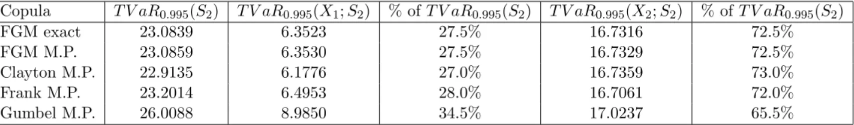
Suppose that X1 and X2 are exponentially distributed with parameters λ1 = 1/2 and λ2 = 1/3 respectively. The dependence between these two risks is defined by the bivariate FGM copula with parameter θF GM = 0.8. This value of θF GM implicates a correlation of 0.2 between X1 and X2. Figure1in the appendix illustrates the accuracy of the approximations of the cdf of S2when using the three discretization methods. Indeed, the decrease of the discretization span h implicates a convergence of the discretized cdf to the real one.
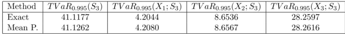
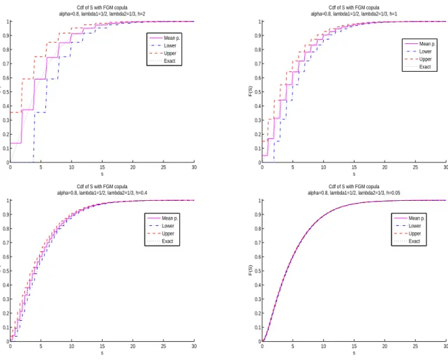
The discretization methods allow an approximation of the cdf of S2 with any copula. We illustrate the use of the FGM, the Clayton, the Frank and the Gumbel copula. The copulas’ parameters are chosen such that we have the same coefficient of correlation between X1 and X2. Figure2in the appendix shows the impact of the copulas on the cdf of S2 which is discretized with the mean preserving method when the correlation coefficient is fixed at 0.2. The first graph displays the drawing of the approximated cdf’s of S2. We then do the difference between a dependent cdf and the independent cdf and trace this difference for the FGM, the Frank, the Clayton and the Gumbel copula in the second graph of Figure 2. These two graphs highlight the fact that the Clayton copula introduces dependence in lower values and that the Gumbel copula permits dependence in the upper queue.
In Figure3 in the appendix, we trace the differences between the TVaR of S2 using dependent risks with one of the copulas discussed before and the TVaR of S2 using the independent copula against the risk level κ. This is done for three increasing values of correlation between X1 and X2. Given that the FGM copula only allows weak dependence it just appears on the first graph. The graphs confirm the fact that the Gumbel copula introduces dependence in high values.
Tables 4 and 5 expose the numerical results for the TVaR and the TVaR-based allocation for
X1 and X2 with the four copulas discussed above and confidence levels equal to 0.99 and 0.995. The calculations are done with the mean preserving discretization method with span h = 0.05 for the four copulas and also with the exact expression for the FGM copula. The tables attest the good precision of the approximation method and confirm the high dependence values inserted by the Gumbel copula.
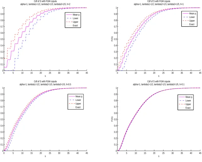
5.3.2 Trivariate case
We illustrate here the difference between the exact and the approximated methods with three risk variables dependent through a trivariate FGM copula. Suppose that X1, X2 and X3 are exponentially distributed with parameters λ1 = 1/2, λ2 = 1/3 and λ3 = 1/5 respectively. The
Copula T V aR0.99(S2) T V aR0.99(X1; S2) % of T V aR0.99(S2) T V aR0.99(X2; S2) % of T V aR0.99(S2) FGM exact 20.9561 6.0998 29.1% 14.8563 70.9% FGM M.P. 20.9574 6.1003 29.1% 14.8571 70.9% Clayton M.P. 20.7918 5.9419 28.6% 14.8499 71.4% Frank M.P. 21.0612 6.2158 29.5% 14.8454 70.5% Gumbel M.P. 22.9669 7.7988 34.0% 15.1682 66%
Table 4: TVaR and TVaR-based allocation for S2 with κ = 0.99.
Copula T V aR0.995(S2) T V aR0.995(X1; S2) % of T V aR0.995(S2) T V aR0.995(X2; S2) % of T V aR0.995(S2) FGM exact 23.0839 6.3523 27.5% 16.7316 72.5% FGM M.P. 23.0859 6.3530 27.5% 16.7329 72.5% Clayton M.P. 22.9135 6.1776 27.0% 16.7359 73.0% Frank M.P. 23.2014 6.4953 28.0% 16.7061 72.0% Gumbel M.P. 26.0088 8.9850 34.5% 17.0237 65.5%
Table 5: TVaR and TVaR-based allocation for S2 with κ = 0.995.
and k ̸= j are all fixed to 1. As for the bivariate case, we show in Figure 4 of the appendix the convergence to the real cdf of S3 of the discretized cdf’s when using the three discretization methods.
Tables 6 and 7 compare the numerical results for the TVaR and the TVaR-based allocation for the three risks with confidence levels equal to 0.99 and 0.995 between exact expressions and approximated results using the mean preserving discretization method with span h = 0.3. As for the bivariate case, they show a satisfying accuracy of the approximation method.
Method T V aR0.99(S3) T V aR0.99(X1; S3) T V aR0.99(X2; S3) T V aR0.99(X3; S3)
Exact 37.5988 4.1726 8.4033 25.0230
Mean P. 37.6062 4.1760 8.4060 25.0243
Table 6: TVaR and TVaR-based allocation for S3 with κ = 0.99.
6
Conclusion
This paper introduces the use of copulas in TVaR-based capital allocation. We obtain explicit expressions for the TVaR and TVaR-based allocation for risks that have exponential and mixture of exponentials distributions linked by a FGM copula. The handy form of this copula permits a direct calculation of the coherent risk measure and its decomposition when we suppose only two different risks. In the multivariate situation, we use divided differences as in Chiragiev and Landsman
(2007). For other copulas, we present approximations for the TVaR and the TVaR-based allocation using three discretization methods for continuous distributions.
Method T V aR0.995(S3) T V aR0.995(X1; S3) T V aR0.995(X2; S3) T V aR0.995(X3; S3)
Exact 41.1177 4.2044 8.6536 28.2597
Mean P. 41.1262 4.2080 8.6567 28.2616
Table 7: TVaR and TVaR-based allocation for S3 with κ = 0.995.
Acknowledgements
The authors acknowledge the Natural Sciences and Engineering Research Council of Canada and the Chaire d’actuariat de l’Universit Laval for their support. This work has also been partially supported by the French Research National Agency (ANR) under the reference ANR-08-BLAN-0314-01. The authors would like to thank an anonymous referee for her/his comments.
APPENDIX
0 5 10 15 20 25 30 0 0.1 0.2 0.3 0.4 0.5 0.6 0.7 0.8 0.9 1 Cdf of S with FGM copula alpha=0.8, lambda1=1/2, lambda2=1/3, h=2s F(S) Mean p. Lower Upper Exact 0 5 10 15 20 25 30 0 0.1 0.2 0.3 0.4 0.5 0.6 0.7 0.8 0.9 1 s F(S) Cdf of S with FGM copula alpha=0.8, lambda1=1/2, lambda2=1/3, h=1
Mean p. Lower Upper Exact 0 5 10 15 20 25 30 0 0.1 0.2 0.3 0.4 0.5 0.6 0.7 0.8 0.9 1 Cdf of S with FGM copula alpha=0.8, lambda1=1/2, lambda2=1/3, h=0.4
s F(S) Mean p. Lower Upper Exact 0 5 10 15 20 25 30 0 0.1 0.2 0.3 0.4 0.5 0.6 0.7 0.8 0.9 1 Cdf of S with FGM copula alpha=0.8, lambda1=1/2, lambda2=1/3, h=0.05
s F(S) Mean p. Lower Upper Exact
0 5 10 15 20 25 30 0 0.1 0.2 0.3 0.4 0.5 0.6 0.7 0.8 0.9 1
Cdf of S with disc. mean p. and corr(X1,X2)=0.2 lambda1=1/2, lambda2=1/3 FGM Frank Clayton Gumbel 0 5 10 15 20 25 30 −0.02 −0.01 0 0.01 0.02 0.03 0.04 0.05 0.06
Difference of cdf of S with independent copula corr(X1,X2)=0.2, lambda1=1/2, lambda2=1/3, h=0.05
s F(S)−F ind (S) FGM Frank Clayton Gumbel
0 0.1 0.2 0.3 0.4 0.5 0.6 0.7 0.8 0.9 1 0 0.5 1 1.5 2 2.5 3 3.5 4
Difference of TVaR of S with independent copula corr(X1,X2)=0.2, lambda1=1/2, lambda2=1/3, h=0.05
kappa TVaR(S)−TVaR ind (S) FGM Frank Clayton Gumbel 0 0.1 0.2 0.3 0.4 0.5 0.6 0.7 0.8 0.9 1 0 1 2 3 4 5 6 7 8 9
Difference of TVaR of S with independent copula corr(X1,X2)=0.75, lambda1=1/2, lambda2=1/3, h=0.05
kappa TVaR(S)−TVaR ind (S) Frank Clayton Gumbel 0 0.1 0.2 0.3 0.4 0.5 0.6 0.7 0.8 0.9 1 0 1 2 3 4 5 6 7 8 9 10
Difference of TVaR of S with independent copula corr(X1,X2)=0.92, lambda1=1/2, lambda2=1/3, h=0.05
kappa TVaR(S)−TVaR ind (S) Frank Clayton Gumbel
0 5 10 15 20 25 30 35 40 45 0 0.1 0.2 0.3 0.4 0.5 0.6 0.7 0.8 0.9 1 Cdf of S with FGM copula alpha=1, lambda1=1/2, lambda2=1/3, lambda3=1/5, h=2
s F(S) Mean p. Lower Upper Exact 0 5 10 15 20 25 30 35 40 45 0 0.1 0.2 0.3 0.4 0.5 0.6 0.7 0.8 0.9 1 Cdf of S with FGM copula alpha=1, lambda1=1/2, lambda2=1/3, lambda3=1/5, h=1
s F(S) Mean p. Lower Upper Exact 0 5 10 15 20 25 30 35 40 45 0 0.1 0.2 0.3 0.4 0.5 0.6 0.7 0.8 0.9 1 Cdf of S with FGM copula alpha=1, lambda1=1/2, lambda2=1/3, lambda3=1/5, h=0.5
s F(S) Mean p. Lower Upper Exact 0 5 10 15 20 25 30 35 40 45 0 0.1 0.2 0.3 0.4 0.5 0.6 0.7 0.8 0.9 1 Cdf of S with FGM copula alpha=1, lambda1=1/2, lambda2=1/3, lambda3=1/5, h=0.1
s F(S) Mean p. Lower Upper Exact
References
Acerbi, C., Nordio, C., and Sirtori, C. (2001). Expected shortfall as a tool for financial risk management. Working paper.
Acerbi, C. and Tasche, D. (2002). On the coherence of expected shortfall. Journal of Banking &
Finance, 26(7):1487–1503.
Artzner, P., Delbaen, F., Eber, J.-M., and Heath, D. (1999). Coherent measures of risk. Math.
Finance, 9(3):203–228.
Asmussen, S. (2000). Matrix-analytic models and their analysis. Scand. J. Statist., 27(2):193–226. B¨auerle, N. and M¨uller, A. (2006). Stochastic orders and risk measures: consistency and bounds.
Insurance Math. Econom., 38(1):132–148.
Cai, J. and Li, H. (2005). Conditional tail expectations for multivariate phase-type distributions.
J. Appl. Probab., 42(3):810–825.
CEIOPS (2006). Choice of risk measure for solvency purposes.
http://ec.europa.eu/internal market/insurance/docs/2006-markt-docs/2534-06-annex-ceiops en.pdf.
CEIOPS (2007). Draft advice to the European Commission in the framework of the Solvency II Project on pillar I issues - further advice. Consultation paper N20. http://www.ceiops.eu/media/files/consultations/consultationpapers/CP20/CP20.pdf.
Chiragiev, A. and Landsman, Z. (2007). Multivariate pareto portfolios: Tce-based capital allocation and divided differences. Scand. Actuar. J., (4):261–280.
Denuit, M., Dhaene, J., Goovaerts, M. J., and Kaas, R. (2005). Actuarial Theory for Dependent
Risks: Measures, Orders and Models. Wiley, New York.
Dhaene, J., Henrard, L., Landsman, Z., Vandendorpe, A., and Vanduffel, S. (2008). Some results on the cte-based capital allocation rule. Insurance Math. Econom., 42(2):855–863.
Embrechts, P. and Puccetti, G. (2007). Fast computation of the distribution of the sum of two dependent random variables. Working paper.
Feldmann, A. and Whitt, W. (1998). Fitting mixtures of exponentials to long-tail distributions to analyze network performance models. Performance Evaluation, 31(3-4):245–279.
Furman, E. and Landsman, Z. (2005). Risk capital decomposition for a multivariate dependent gamma portfolio. Insurance Math. Econom., 37(3):635–649.
Furman, E. and Landsman, Z. (2007). Economic capital allocations for non-negative portfolios of dependent risks. Proceedings of the 37-th International ASTIN Colloquium, Orlando.
Gatfaoui, H. (2005). How does systematic risk impact us credit spreads ? a copula study. Bankers
Markets & Investors, 77:5–12.
Keatinge, C. L. (1999). Modeling losses with the mixed exponential distribution. In Proceedings of
the Casualty Actuarial Society, volume 86, pages 654–698.
Khayari, R. E. A., Sadre, R., and Haverkort, B. R. (2003). Fitting world-wide web request traces with the em-algorithm. Performance Evaluation, 52(2-3):175 – 191. Internet Performance and Control of Network Systems.
Kim, H. T. (2007). Estimation and allocation of insurance risk capital. PhD thesis, University of Waterloo.
Klugman, S. A., Panjer, H. H., and Willmot, G. E. (2008). Loss models: From data to decisions. Wiley Series in Probability and Statistics. John Wiley & Sons Inc., Hoboken, NJ, third edition. Landsman, Z. M. and Valdez, E. A. (2003). Tail conditional expectations for elliptical distributions.
N. Am. Actuar. J., 7(4):55–71.
M¨uller, A. and Scarsini, M. (2001). Stochastic comparison of random vectors with a common copula. Math. Oper. Res., 26(4):723–740.
M¨uller, A. and Stoyan, D. (2002). Comparison methods for stochastic models and risks. Wiley Series in Probability and Statistics. John Wiley & Sons Ltd., Chichester.
Nelsen, R. B. (2006). An introduction to copulas. Springer Series in Statistics. Springer, New York, second edition.
Neuts, M. F. (1981). Matrix-geometric solutions in stochastic models, volume 2 of Johns
Hop-kins Series in the Mathematical Sciences. Johns HopHop-kins University Press, Baltimore, Md. An
algorithmic approach.
Panjer, H. H. (2002). Measurement of risk, solvency requirements and allocation of capital within financial conglomerates. Institute of Insurance and Pension Research, University of Waterloo, Research Report 01-15.
Schmock, U. (2006). Modelling dependent credit risks with extensions of creditrisk+ and appli-cation to operational risk. Lecture notes, PRisMa Lab, Institute for Mathematical Methods in Economics, Vienna University of Technology.
Schmock, U. and Straumann, D. (1999). Allocation of risk capital and performance measurement. Talk at the Conference on Quantitative Methods in Finance, Sydney, Australia.
Tasche, D. (1999). Risk contributions and performance measurement. Working paper, Technische Universitt Mnchen.
Wang, S. S. (2002). A set of new methods and tools for enterprise risk capital management and portfolio optimisation. Working paper, SCOR Reinsurance Company.
Yeo, K. L. and Valdez, E. A. (2006). Claim dependence with common effects in credibility models.