Uncertainty Assessment for Management of Soil Contaminants with Sparse Data

Contaminants with Sparse Data

OLAF TIETJE

ROLAND W. SCHOLZ

Chair of Environmental Science - Natural and Social Science Interface

Swiss Federal Institute of Technology Haldenbachstr. 44

8092 Zurich, Switzerland

ABSTRACT / In order for soil resources to be sustainably managed, it is necessary to have reliable, valid data on the spatial distribution of their environmental impact. However, in practice, one often has to cope with spatial interpolation achieved from few data that show a skewed distribution and uncertain information about soil contamination. We present a case study with 76 soil samples taken from a site of 15 square km in order to assess the usability of information gleaned from

sparse data. The soil was contaminated with cadmium pre-dominantly as a result of airborne emissions from a metal smelter. The spatial interpolation applies lognormal anisotropic kriging and conditional simulation for log-transformed data. The uncertainty of cadmium concentration acquired through data sampling, sample preparation, analytical measurement, and interpolation is factor 2 within 68.3 % confidence. Uncer-tainty predominantly results from the spatial interpolation ne-cessitated by low sampling density and spatial heterogeneity. The interpolation data are shown in maps presenting likeli-hoods of exceeding threshold values as a result of a lognor-mal probability distribution. Although the results are not deter-ministic, this procedure yields a quantified and transparent estimation of the contamination, which can be used to delin-eate areas for soil improvement, remediation, or restricted area use, based on the decision-makers’ probability safety requirement.

Land-use management is challenging for the plan-ning departments of both local and regional govern-ments, especially where land use is extensive and con-taminants are widespread (Roe and van Eeten 2001). Low concentrations of pollutants have long-term im-pacts, e.g., on soil fertility in the case of soil contami-nants (Grunewald 1997; Gysi and others 1991). The impact of contaminants contributes to a shortage of usable land and consequently to competition of interest among different land uses. As a result, the market value of usable land may change and thus affect sustainable land-use management as Prato (2000) demonstrated.

We present a case study involving a location with cadmium-contaminated soil. For a large part of the area considered, soil measurements show contamination lev-els above the guide value, but below the remediation value as outlined in the Swiss Ordinance Relating to Pol-lutants in Soil (VBBo 1998) (Tables 1 and 2). If the guide value is exceeded, remediation of the soil may be considered appropriate where contamination of groundwater, crops, or soil fertility could be

endan-gered. However, in this case, there are no standards mandating a cleanup. According to Swiss Ordinance Re-lating to Pollutants in Soil (VBBo 1998) soil contamina-tion levels between the guide value and remediacontamina-tion value indicate the necessity of a change in land use, for example, from food production to residential use. Such changes often provide a less expensive alternative to remediation. Remediation is only legally obligatory when the remediation value is exceeded. This legal situation shows that assessment of soil contamination is relevant for sustainable land management, even when the pollutants pose no risk to human health. Assess-ment of soil contamination for precautionary soil im-provement is difficult, because of the lack of data and high degree of uncertainty from sparse data. Decisions on soil use change are difficult to substantiate. In order to evaluate the affected areas in a valid, reliable, and cost-effective way, a spatial interpolation that includes appropriate uncertainty information is required.

The common sources of uncertainty in spatial pre-diction are data sampling (sparseness and inaccuracy), the preparation and measurement of samples in the laboratory (Dubois and Schulin 1993, Muntau and oth-ers 2001), the spatial interpolation of the data (Goo-vaerts 2001, Meuli 1997), and subsequent modeling (Hendriks and others 2000, Keller and others 2001, 2002). Several geostatistical models address the amount of uncertainty from interpolation techniques (Barabas

KEY WORDS: Conditional simulation; Lognormal ordinary kriging; Un-certainty assessment; Probability of occurrence; Sparse data

Published online June 29, 2004.

*Author to whom correspondence should be addressed, email: schnabel@nsl.ethz.ch

and others 2001, Bouma and others 1996, von Steiger and others, 1996). Modeling uncertainty by means of stochastic simulation is also widely used (Gotway and Rutherford 1993, Pan 1997, Van Meirvenne 2001). For example, Goovaerts (2001) compared kriging-based es-timation to simulation-based spatial eses-timation and concluded that simulation offers several advantages, the most important one being that it provides a model of spatially local uncertainty. In cases of lognormally distributed data, ordinary lognormal kriging is easy to implement and yields better results than other kriging methods (Papritz and Moyeed 1999, Saito and Goo-vaerts 2000). Other investigations applied indicator kriging (Van Meirvenne 2001, Webster and Oliver 2001) or disjunctive kriging (Papritz and Moyeed 1999, von Steiger and others 1996), because of the complica-tions to estimating the local probability density func-tion when applying a tradifunc-tional backtransformafunc-tion (Geovariances 1997, Webster and Oliver 2001, p. 19). Therefore, we follow the approach of Limpert and others (2001), who presented the uncertainty on the

raw scale by means of the geometric mean, the multi-plicative standard deviation, and consequently, the multiplicative confidence intervals for a multitude of lognormal-distributed data.

Thompson and Fearn (1990, p. 271) discuss the relation between sampling and cost of analysis as well as the quality of data appropriate for data assessment. They define fitness for purpose as “the property of data, produced by a measurement process, that enables a user of the data to make technically correct decisions for a stated purpose.” The decision whether or not the information supplied by the available data and its de-gree of uncertainty are useful depends on the purpose for which the data will be used. Decision-makers have to judge the appropriateness of using uncertainties as a substantive base for their decision (Ramsey and others 1998, Thompson 1995). It is the decision and its con-sequences that matter, rather than the accuracy of the prediction (Goovaerts and Meirvenne 2001). Thus, the main objective of this study is to analyze the usability of the information given by spatial interpolation of few measurements, combined with probabilistic reasoning based on sparse data for the case of Dornach (Canton Solothurn, Switzerland). The following questions will be addressed:

● What kind of spatial prediction is suitable when distant, irregularly distributed measurements are analyzed for environmental management purposes? ● How can the uncertainty in an interpolation be best

assessed and presented?

● What possibilities and limitations are posed by ap-plying the interpolation method and its resulting uncertainty for practical planning purpose?

Data

We present a case study from Switzerland where 76 soil samples were taken in an area of 15 square kilome-ters. Each was a composite sample from topsoil (20 cm depth) within a range of 10 square meters (Wirz and Winisto¨rfer 1987). Soil samples were taken without a specific sample design, and the sites were more or less randomly distributed. An attempt was made to cover the supposed area of contamination (Figure 1) and take local circumstances into account.

The total heavy metal content of the soil was deter-mined in a 2 M HNO3extract following the Swiss

Ordi-nance Relating to Pollutants in Soil (VBBo 1998) and measured with a atom adsorption spectrometer (AAS) using the flame-AAS method.

The data analysis in Table 2 reveals that the distri-bution of heavy metal measurements is highly skewed Table 1. Legal threshold values for remediation of

cadmium in soil in Switzerland (VBBo 1998) Swiss Ordinance Relating to

Pollutants in Soil Cadmium total, HNO3soluble (mg/kg) Guide Value 0.8 Trigger Value

Use with probable oral intake 10

Use for food planting 2

Use for feed planting 2

Remediation Value

Agriculture and horticulture 30

Gardening 20

Playgrounds 20

Table 2. Statistical properties of the data

Value Cd (mg/kg) in Cd (mg/kg) Count 76 76 Geometric mean 0.93 ⫺ Arithmetic mean 1.43 ⫺0.08 Standard deviation 2.69 0.80 Variance 7.26 0.64 exp {average [ln(Cd)]} 0.93 ⫺ exp {stddev[ln(Cd)]} 2.22 ⫺ Median 0.86 ⫺0.16 exp{median[ln(Cd)]} 0.86 ⫺ Skewness 7.36 0.78 Kurtosis 59.67 2.89 Min 0.12 ⫺2.12 Max 23.3 3.15

(skewness 7.36). This also shows the difference between the arithmetic mean (1.43 mg/kg) and the geometric mean (0.93 mg/kg) of the raw data. For such data, logarithmic transformation may be appropriate before interpolation. The statistics from a Kolmogorov-Smir-nov test show that the logarithmically transformed data follow a normal distribution (Pⱖ 0.35, Table 3).

Be-cause the test presumes independency of the observa-tions, a random set from the data, chosen with the most possible distance from every other measurement point, was also tested and accepted (P⫽ 0.74, Table 3).

Cadmium was emitted from a metal smelter during the past century. Today the pollutant can be found on the west side of Dornach (Figure 1), a result of the Figure 1. Spatial distribution of sampling points in Dornach (Canton Solothurn, Switzerland).

Table 3. Test of normality with a one-sample Kolmogorov-Smirnov test for the logtransformed dataa

Cd (mg/kg) Ln(Cd) (mg/kg) Ln(Cd) (mg/kg)a

N 76 76 29

Normal parameters

Mean 1.43 ⫺0.08 ⫺0.06

SD 2.69 0.80 0.98

Most Extreme Differences

Absolute 0.31 0.11 0.13

Positive 0.30 0.11 0.13

Negative ⫺0.31 ⫺0.06 0.13

Kolmogorov-Smirnov Z 2.74 0.94 0.68

Asymp. Sig. (2-tailed) 0.00 0.35 0.74

a

A subsample of spatial independent data fulfill the assumption of independency (test distribution is normal, mean and standard deviation are calculated from data).

west-to-east dominant wind direction (Schweizerische Meteorologische Anstalt 1982–91) and the northwest facing slope on which the community of Dornach was built (Hesske and others 1998). In addition to the airborne contamination, the cadmium content in par-ent material is about the Swiss average of 0.3 mg/km of soil (Tuchschmid 1995, Keller 2001).

Geiger and Schulin (1995) found high variability (N ⫽ 50, average ⫽ 4.38 mg/kg, variance 0.72 (mg/kg)2_,

min ⫽ 2.37 mg/kg, max ⫽ 5.92 mg/kg) on a 40 m transect in the same area. Soil parameters and contam-inants tend to behave randomly on the small scale (Webster 2000). Thus, for this case study, it was neces-sary to take the variability of the data on a scale of a few tens of meters into account when we analyzed it.

Methods

Within the framework of geostatistical analysis, the measured cadmium concentrations (see above) are as-sumed to be one realization of a stochastic process {Z(x): x僆 D} (Cressie 1993, Goovaerts 1997), where D denotes the sample space for the investigated case study area of Dornach (Figure 1). Let x1,...,xndenote the data

coordinates and Z (x1),...,Z(xn) the logarithms of the

measured cadmium concentrations of the 76

measure-ments. Then, the difference Z (x)⫺ Z(x ⫹ h) with x, x ⫹ h 僆 D depends on the distance vector h (Matheron 1963). This dependency is expressed by means of the semivariance␥ (h), which is defined as half the variance of concentration differences of all data pairs with the same distance h (Journel 1989). The range r — the spatial dependency — indicates the maximum distance between sites, beyond which concentrations are consid-ered to be uncorrelated. Properties and characteristics of this function are discussed in geostatistical textbooks (e.g., Cressie 1993, pp. 58ff).

Analysis of spatial dependency

The spatial dependency of the cadmium concentra-tions is empirically investigated using standard geostatistical software (Geovariances 1997). The inves-tigation includes the (supposed) total area of contam-ination.

A variogram map (see Figure 2) of the logarithmi-cally transformed cadmium data shows an empirical semivariance function, which depends on the length and direction of distance vector h. It shows that in the southeast direction the range is larger than in other directions. This indicates that an anisotropic semivari-ance should be considered. For the variogram model we used a spherical function (Figure 3), which is ex-pressed as (equation 1):

Figure 2. Variogram map of the logarithmically transformed cadmium data. Each grid cell shows the semivarince of the lag vector (x,y). D1–D4 indicate the direction of the anisotropic variograms.

␥共h,␪ 兲 ⫽ c0⫹ c1

再

冋

册

冎

the sill; and ⍀共␪兲 ⫽ 关A2_cos2_{共␪ ⫺ ␣兲 ⫹ B}2_sin2_共␪ ⫺ ␣兲兴12 , which defines the geometric anisotropy by means of an ellipsoid with angle ␣, the direction in which the continuity is greatest; A, the maximum diam-eter; and B, the minimum diameter, which is perpen-dicular to A (Webster and Oliver 2001). This express the so-called geometric anisotropy, for which the range (but not the sill) depends on the direction. Referring to the variogram map, the direction␣ of the largest diam-eter is set to⫺65° (155° in geographical notation; see Figure 2). Other kinds of semivariance functions (like Gaussian or exponential) and zonal anisotropy are dis-cussed by Journel and Huijbregts (1978) and Matheron (1963).

Further, for the analysis of spatial contamination pattern, trend models for the components of distance to the metal smelter (d) and deviation from the domi-nant wind direction (⌬␪) are used as suggested by Saito and Goovaerts (2001). Trend factors are fitted with five different regressions and residues are used to predict the spatial dependency. Hereafter the mean square

error (MSE) from cross validation (Goovaerts 2001, Armstrong 1998) indicates the goodness of prediction with a trend.

Ordinary Kriging

The interpolation applies an ordinary kriging method, where the data are logarithmically trans-formed before kriging, and then transtrans-formed back af-terwards. Lognormal ordinary kriging interpolates by means of a weighted average (equation 2):

Z*(x0)⫽

冘

i⫽ 1 n

␭iZ共 xi兲 (2)

where Z* (x0) is the estimated value at point x0, Z (xi) is

the measured value at xi, and␭iare the weights (adding

up to 1). Nearby measurements are considered to be more correlated to the estimation point and, therefore, carry a higher weight than more distant measurements. A moving (ellipsoidal) neighborhood is defined by the parameters of anisotropy, i.e., a rotation of␣ ⫽ -65° and a range of A⫽ 900 m (direction D1, D2) and B ⫽ 500 m (direction D3, D4). This distributes the weight of the sampling points along the preferred direction, thus emphasizing the local spatial structure of contamina-tion.

The kriging variance ␴Zi 2

(x0) is computed as the

weighted sum of the estimation point (x0) and the

measured points (Equation 3). The kriging variance is then

Figure 3. Anisotropic variograms in the directions D1–D4; their ranges are 900 m to 500 m, the nugget effect is 0.13 (mg/kg)2_{, and}

the sill is 0.53 (mg/kg)2_{. Number}

of pairs and lag value for each lag are shown in the annotations.

␴Z2⬘ 䡠 共 x0兲 ⫽

冘

i⫽ 1 n

␭i␥共 xi, x0兲 ⫹ ␺共 x0兲 (3) Where ␭(xix0) is the semivariance between the data

point xiand the estimation point x0. The weights␭iare

distributed in terms of the data model (see above) and under the requirement of unbiasedness. ␺(x0) is the

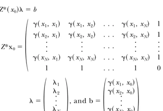
Lagrange multiplier used for minimization of the krig-ing variance (Cressie 1993, Journel 1989). The krigkrig-ing system is given in detail in the annotations.

After kriging, the lognormal estimates are trans-formed back to the original scale. Several back-trans-formations methods have been proposed (Cressie 1993, p. 136, Saito and Goovaerts 2000, Webster and Oliver 2001, p. 180). We transformed the values back accord-ing to equation 4:

Z*r⫽ exp

冉

␴Z*

2

2

冊

where Z*r is the estimated value in the raw scale, Z* is

the estimated value, and␴Z

Zi, is the kriging variance, all

on the logarithmic scale. For the kriging variance the transformation (Limpert and others 2001, Stahel, 2000, p. 136) is (equation 5): ␴Z*r 2_{⫽ m} reSr 2 共1 ⫺ e⫺ ␴Z* 2 兲 (5)

where mris the mean, sr 2

is the dispersion variance of the raw variable, and␴Zi

2

is the kriging variance (on the log scale)(Geovariances 1997). For the statistical char-acterization of the interpolated data, we calculated the median of the raw variable given the mean Z* on the log scale as Zr

M_{共x兲 ⫽ exp关Z*共x兲兴 (median of the raw}

variable) and the multiplicative standard deviation from the untransformed kriging variance ␴Zi2 on the

log scale as␴ (x) ⫽ exp[␴Zm(x)] (Limpert and others

2001, Stahel, 2000, p. 136). Please note that ZP

is the median (and not the mean) of the raw variable and that the multiplicative standard deviation (sometimes called the geometric standard deviation) is calculated as the exponential of the standard deviation ␴Zi on the log

scale (and not as the exponential of the variance on the log scale).

Geostatistical conditional simulation To characterize the small-scale variability without a smoothing effect, a random realization of a stochastic process is generated. The idea is to compute a multitude of such random realizations and characterize the distribution at each estimation point through the average and standard deviation. All calculations are conducted using the log-arithmically transformed data.

The stochastic simulation was performed using the turning bands method (Matheron 1963, Tietje 1993),

which is one of the two available methods [as sequential Gaussian simulation (Deutsch and Journel 1998)]. The turning bands method simulates realizations of a one-dimensional Gaussian process [Y (tu): t僆 R] along the L lines L1,...,LLthrough the origin defined by the unit

vectors u៮1,...,u៮L. The lines all have the same arbitrary

origin (Gotway 1994) and are uniformly distributed within the (in this case) 2-dimensional space. If u1,...,uL

are unit vectors in the direction L1,...,LL, the simulated

value Zs(x), x僆 D, is an average of those values, which

are generated at the orthogonal projection tui(x) of the

terminal point x onto the line of direction uជi,兵Y关ui共x兲*uជi兴:i ⫽ 1,…,L其. Finally, the generated value

at point x is (equation 6): Zs共 x兲 ⫽ 1 兹Li

冘

A detailed discussion of the method can be found in Gotway (1994) and Journel (1974). Conditioning the simulation means to force the simulated surface to pass through the measurements. Hence, the simulated value is obtained through the formula (Journel and Hui-jbregts 1978) (equation 7):

Z*cs共 x兲 ⫽ Z*共 x兲 ⫹ 关Zs共 x兲 ⫺ Z*s共 x兲兴 (7)

where Z*(x) is the kriged value obtained from the data Z(xi), (measurements i⫽ 1,...,n), Zs(x) is the simulated

value from equation 6, and Z*s共x兲 is a kriged value

obtained from Zs (xi) using the realizations at the

coordinates of the measurements. The conditional simulation was conducted with 100 turning bands for each of 100 realizations at each gridpoint x僆 D. A simulation postprocessing averages the results of sim-ulations according to equation 7 for each grid node

Zcs ␮_{共 x兲 ⫽} 1 100

冘

At each gridpoint x僆 D the mean is used to inter-polate the cadmium concentration, and the standard deviation ␴*cs共 x兲 ⫽

冑

冘

Zcs

M_{共 x兲 ⫽ exp关Z*}

cs共 x兲] (10)

which is median of conditional simulation of the raw variable and

which is standard deviation of conditional simulation of the raw variable.

Uncertainty assessment To assess the overall uncer-tainty of the interpolated concentrations, we consider the following sources of error: soil sampling, sample preparation for analytical measurement, analytical measurement itself, and interpolation. One model for these sources of error is the sum of variances induced throughout the assessment. Following the approach of the Analytical Methods Committee (1995) and Ramsey and Argyraki (1997), we assume the uncertainty U(x) (equation 12) as random field

U共 x兲 ⫽ ␴constant2 ⫹ V (x) for all x 僆 D (12) which includes a constant part␴2

constantand a spatially

variable part V(x). V(x) indicates the error due to inter-polation and ␴2

constant indicates the uncertainty

in-duced by soil sampling and measuring. The latter is considered to be the sum of the uncertainties of soil sampling (sampling pattern, density, composite, or spot sample), preparation of the soil sample (fragment re-moval, drying, grinding, sieving, splitting), and mea-surement of the cadmium content [flame-atom-spec-trometer (AAS)] itself (Muntau and others 2001, Theocharopoulos and others 2001) (equation 13). ␴constant 2 _{⫽ ␴} sampling 2 _{⫹ ␴} samplingpreparation 2 _{⫹ ␴} measurement 2 (13) The project “European methods in soil sampling” (CEEM) (Desaules and others 2001, Wagner and others 2001a) has evaluated the sources of uncertainty in soil pollutants assessment. It demonstrated that sampling and/or sampling preparation are the main sources of uncertainty, to the degree of which depends on the element analyzed and its concentration level (Wagner and others 2001b). Moreover, the investigation empha-sized the deviation from sampling being higher than the analytical deviations. This is especially true for cad-mium. From the results of the CEEM project, we de-rived an uncertainty of 0.3 mg/kg for sampling and sampling posttreatment for the constant part of the overall uncertainty (␴2

constant) (Wagner and others

2001b, p. 87). This uncertainty might also be caused by the use of different sampling techniques (with varia-tions in sampling depth, sieving, etc.), the presence of small-scale heterogeneity [about 40% (see Wagner and others 2001b, p. 92)], and diversity of conditions asso-ciated with type of land use [variation coefficients of 8.1 %, 7.2 %, and 2.7 % for forest, agriculture, and grass-land use (Desaules and others 2001)]. Von Holst (1997) claims that sampling itself causes the highest degree of error followed by sampling preparation. Wa¨chter (1997) even infers that the error of the

mea-surement instruments is negligible relative to the high error influence of sampling.

Concerning the spatially variable part of the uncer-tainty [V(x), equation 8], the geostatistical theory (Arm-strong 1998, Webster and Oliver 2001) states that the kriging variance is zero at measurement points and minimized (equations 2 and 3) between the sampling points. The magnitude of the kriging variance, there-fore, depends on the distribution of the sampling points (note that the kriging characteristics — neigh-borhoods, anisotropy, the support, etc. — have to be set carefully). Because the sampling in the investigated area is sparse, large parts of the investigated area are expected to show a high kriging variance. The maxi-mum of the kriging variance is related to the sill of the variogram and hence depends on the overall variance of the data (see above).

Finally, the overall uncertainty is calculated as U(x)⫽exp (In 1.35⫹1n␴v(x)), which is used to

esti-mate the spatially distributed uncertainty. Due to the geometric distribution (and hence the multiplicative confidence intervals) of the results, it is called the uncertainty factor throughout the text. In conclu-sion, the probability of exceeding a threshold of concentration C is estimated by solving equation 14: P共Z* ⬎ C兲 ⫽ 1 ⫺ ␾关共ln C ⫺ Zlog*兲/␴u共 x兲兴 (14) for the probability pxof the standard normal

distribu-tion␾.

Results

Spatial Estimation

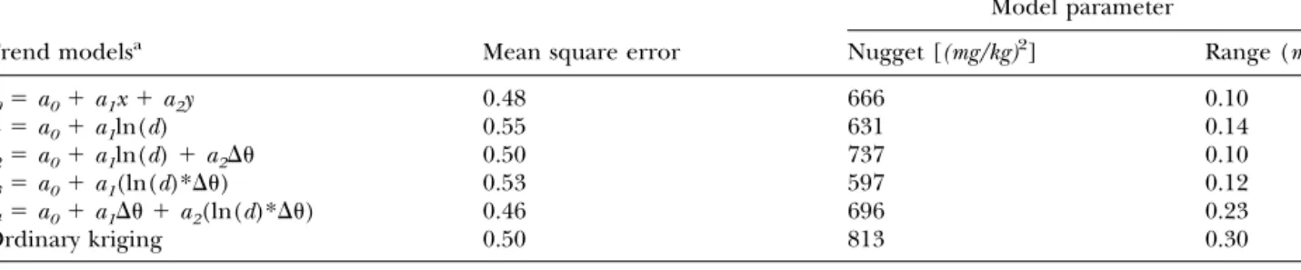
The estimation of the spatial distribution of the cadmium concentration relies on the geostatistical analysis of the data. The trend analysis reveals no sig-nificant spatial trend. Besides a linear trend (Webster and Oliver 2001), the distance to the metal smelter and/or the main wind direction is additionally com-puted as regression parameters (Saito and Goovaerts 2001). Residues from regression are used for kriging and cross validation. Table 4 shows the mean square error of prediction with these trends compared to or-dinary kriging without a trend. The results of Table 4 justify a spatial prediction without a trend in the inves-tigated area.

Spherical models are suitable for both empirical variograms (Table 5, equation 1, and the isotropic spherical function is given in the annotations). In both cases, the sill approximately equals the data variance. The anisotropic and isotropic variograms on the log scale are shown in Figures 3 and 4. For the

interpola-tion of cadmium, we use the anisotropic model dis-played in Figure 3, because the variability of the cad-mium contents depend on direction, as shown in the variogram map in Figure 2. The range is from 500 m to 900 m, encompassing the range of the isotropic model. The anisotropic model is computed for lag classes of

230 m and is discontinuous near the origin showing a nugget effect of 0.125 (mg/kg)2 (log scale).

The interpolated cadmium concentrations are dis-played in Figure 5, which is a cutout of the lated area. The statistical properties of the interpo-lations (isotropic and anisotropic) and the Figure 4. Isotropic variogram with a range of 813 m, a nugget effect of 0.297 (mg/kg)2_{, and a sill of 0.332}

(mg/kg)2_.

Table 4. Mean square error from cross validation for five different trend models and ordinary kriging (isotropic variogram) for 76 data points

Model parameter

Trend modelsa _{Mean square error Nugget [(mg/kg)}2_{] Range (m)}

t0⫽ a0⫹ a1x⫹ a2y 0.48 666 0.10 t1⫽ a0⫹ a1ln(d) 0.55 631 0.14 t2⫽ a0⫹ a1ln(d)⫹ a2⌬␪ 0.50 737 0.10 t3⫽ a0⫹ a1(ln(d)*⌬␪) 0.53 597 0.12 t4⫽ a0⫹ a1⌬␪ ⫹ a2(ln(d)*⌬␪) 0.46 696 0.23 Ordinary kriging 0.50 813 0.30

a_{(d) denotes the distance to the metal smelter and (⌬␪) is the deviation of wind direction from west to east, x, y are data coordinates. All models}

are calculated in accordance to Saito and Goovaerts (2001). Models of spatial dependency are derived from the residues of regression.

Table 5. Geostatistical properties of the variograms, all data shown on log-scale

Isotropic variogram Anisotropic variogram

Model spherical spherical

Direction omnidirectional four directions, D1-D4

Range 813 m ⫺65° ⫽ 900 m, ⫺20°, ⫹20°, ⫹70° ⫽ 500 m

Nugget effect 0.297 (mg/kg)2 _{0.125 (mg/kg)}2

conditional simulation (anisotropic) are shown in Table 6. Differences between kriging of cadmium with isotropic and anisotropic variograms mainly re-sults from their different nugget effects. The larger nugget effect leads to a smoother isotropic kriging interpolation (Webster and Oliver 2001) with less variance and an underestimation of cadmium con-centrations.

The statistical properties of the anisotropic interpo-lation (Table 7) have been calculated for the area indicated to be the core area in Figure 1.

Uncertainty assessment The uncertainty of factor 2 (two times the estimate by multiplicative standard de-viation) — postulated by the Analytical Methods

Com-mittee (1995), Ramsey and Argyraki (1997), as well as Fresenius and others (1995) — can only be estimated at a probability of 68.3 %, whereas the demand of px ⫽

97.5 % accuracy leads to an uncertainty factor of about 4.2. The uncertainty only decreases in the vicinity of the measurements.

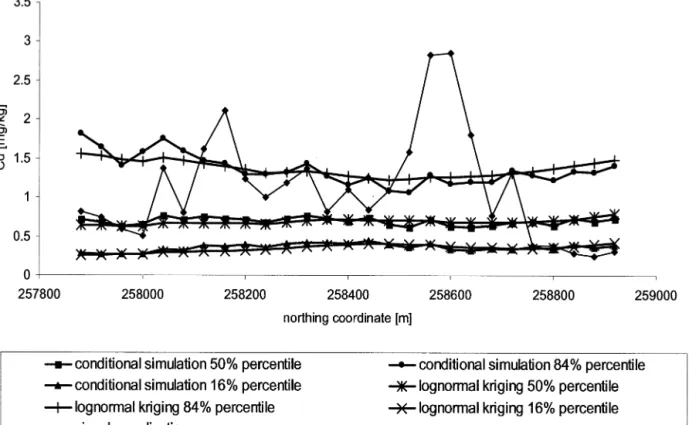
The rationale of the spatially variable part V(x) of the overall uncertainty is illustrated by Figure 6, which shows a north–south transection of Dornach. A single realization of the conditional simulation demonstrates considerable variability and randomly high cadmium concentrations.

As can be seen from Figure 6, in reality some cad-mium concentrations beyond the 68.3 % confidence Figure 5. Spatial distribution of cadmium concentrations in topsoil after conditional simulation. The median of 100 realizations on the raw scale [ZM

cs] is displayed, taken only from the core area indicated in Figure 1.

Table 6. Statistical properties of the interpolations (isotropic and anisotropic) and the conditional simulation Data Isotropic estimation Anisotropic estimation Conditional simulation Counts 76 11,878 10,802 10,802 Geometric mean [e␮mg/kg] 0.93 1.05 1.08 1.09 Standard deviation [e␮mg/kg] 2.22 2.33 2.27 2.33 Minimum [mg/kg] 0.12 0.12 0.12 0.14 Maximum [mg/kg] 23.3 4.36 8.81 9.03

interval of the interpolation and simulation could oc-cur. The results for the spatially variable part are indi-cated in Table 7 as is the geometric standard deviation e␮mg/kg.

Relevance for Decisions on Soil Remediation

To come to any decision, the results of the kriging interpolation and the uncertainty assessment have to be in accordance with the standards set out in the Swiss

Ordinance Relating to Pollutants in Soil (VBBo 1998) (Ta-ble 1). This document contains the three threshold values associated with a long-term fertility goal (guide value), the concentration beyond which a more de-tailed investigation is required (trigger value), and the concentration beyond which a remediation is pre-scribed (remediation value).

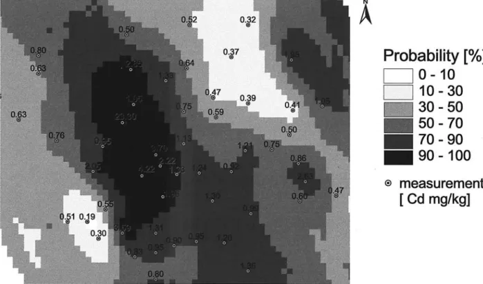
Figure 7 presents the probability of exceeding 2 mg cadmium per kg soil (trigger value for food and feed Figure 6. A south–north transection with the results of one singular realization and some percentiles of the conditional simulation and lognormal kriging. The 50th percentiles are estimated by taking the exponential of the mean values on the logarithmic scale. The other percentiles are calculated as the exponential of the percentiles on the logarithmic scale exp[Zlog*

(x)⫾␾(p)␴log(x)], with the 16th and 84th percentiles of the normal distribution␾(16%) ⫽ ⫺1 and ␾(84%) ⫽ 1.

Table 7. Statistical properties of the interpolation for the core area of pollution (indicated in Figure 1) and the total area of pollution

Anisotropic modeling

Core area Total area

Cadmium estimated Cadmium simulated Cadmium estimated Cadmium simulated Counts 3870 3870 10802 10802 Geometric mean [e␮mg/kg] 1.03 1.03 1.08 1.09 Standard deviation [e␮mg/kg] 1.95 1.97 2.27 2.33 Minimum [mg/kg] 0.28 0.28 0.12 0.14 Maximum [mg/kg] 8.81 9.03 8.81 9.03

planting). Clearly, the probability of any other thresh-old value can be presented. In practice, decision-mak-ers have to agree on a probability statement that they consider reliable and safe enough for the specific case. Figure 6 shows one randomly chosen realization out of a total of 100 realizations that determine the simulated value. As can be seen, some local cadmium concentra-tions at this point exceed the 84th percentile of the prediction. Presentations, as the one demonstrated in Figure 6, facilitate understanding of the meaning and consequences of the results, which are phrased as “there is a 16 % likelihood that a specific cadmium concentration will be exceeded”. In addition, it is pos-sible to delineate corresponding areas, which may be subjected to further investigations (e.g., additional measurements). A combination of the spatially dis-tributed probability of occurrence with other data of a geographic information system (GIS), such as land use classifications, might lead to a valuable decision. However, if a high degree of reliability and confi-dence is required (e.g., 95 %) and the costs of soil treatment are very high, Figure 7 suggests that fur-ther measurements should be collected. In general, knowledge about the probability of exceeding legal threshold values helps to become aware of necessary actions that have to be taken in sustainable soil

im-provement — depending on the decision-makers’ risk level. For the case considered in this study, the following conclusions became evident from the inter-polation and the uncertainty assessment:

● cadmium contamination above legal remediation value (for all kind of uses) is not likely (even with a probability below 50 %) on any side;

● a small area is contaminated above trigger value with a probability of more than 90 %;

● cadmium contamination above guide value is wide-spread with more than 50 % probability;

● high probabilities for cadmium contamination above 0.8 mg/kg are delineated mainly around the emission source; and

● Only a small domain of the case area is not contam-inated above the guide value of Swiss Ordinance related to Soil (VBBo 1998)

Since the contamination from sources such as sew-age sludge or fertilizer is ongoing (Keller and others 2001), decision-makers should also bear in mind that the cadmium concentration might still be accumulat-ing and any kind of soil improvement might help to sustain the multi-functional use of soil (Bouma 2002).

Conclusion

The case study shows that even sparse data are suit-able for an assessment of contaminated land. In our case we state an uncertainty factor of 2 with 68.3 % accuracy and we acknowledge statements such as “The probability that the soil contamination at this point exceeds 2 mg cadmium per kg soil is less than 40 %”. We infer from the preceding analysis that statements of this kind can be given in a reliable way.

For the spatial interpolation of the cadmium con-centrations, a lognormal ordinary kriging (Papritz and Moyeed 1999, Matheron 1963) and a conditional sim-ulation (Goovaerts 2000, Journel 1974) were applied. The ordinary kriging was improved by the application of an anisotropic variogram. The anisotropic variogram shows varying distances of autocorrelation in different directions. Several two dimensional stochastic realiza-tions were produced and a conditional simulation was applied to analyze the local variability. The conditional simulation (as the stochastic realizations are forced to hit the measured data) also yielded an estimation of the local uncertainty. A logarithmic transformation of the data and a back-transformation after interpolation ac-cording to Limpert and others (2001) was used to obtain the geometric mean and the multiplicative stan-dard deviation. The geometric distribution was used to obtain the percentiles of the probability density func-tion and to predict the condifunc-tional cumulative density function including the uncertainty. With this approach, the uncertainties involved in the interpolation are ap-propriately estimated. Hence, this procedure can be applied for uncertainty assessment of lognormally and spatially distributed data.

The uncertainty assessment exemplifies that the main part of the overall uncertainty is due to the sparse-ness of the data that underlies the spatial interpolation. The second important uncertainty is due to the sam-pling and sample preparation. Because corresponding data are hard to obtain (see, e.g., CEEM Project; Wag-ner and others 2001b), we roughly estimated this as 35 % of the estimated cadmium concentration using quan-titative (von Holst 1997, Wa¨chter 1997, Wagner and others 2001b) and qualitative results (Ramsey 1998, Tiktak and others 1999) as a reference. For the purpose of this investigation, other sources of uncertainty, such as the analytical measurement have been determined to be negligible. In conclusion, the resulting overall un-certainty is suitable to identify regions with a high risk of contamination. The interpolation combined with the uncertainty assessment is sufficiently reliable to de-lineate potentially contaminated sites pictured in “maps of probability of occurrence.”

Acknowledgements

The work reported in this paper was conducted in the context of the Integrated Project Soil of the Swiss Priority Program Environment. We are grateful to Mar-tin Fritsch, who initiated the project and guided it until 2000, and to the colleagues at UNS and within the IP Soil for the helpful discussions. We also appreciate the comment of three anonymous reviewers. The project was funded by the Swiss National Science of Founda-tion (Project number 5001-44758) and the Swiss Fed-eral Institute of Technology (Project number 0048-41-2609-5).

Annotations

Table 8 shows the number of pairs and semivari-ances for single lags of the variogram, calculated in equation (1) and shown in Figure 3.

The formal kriging system is: Z*共 x0兲␭ ⫽ b Z*x0⫽

冢

冣

冢

冣

冢

冣

Spherical function calculated for Figure 5 and Table 5 and 6:

Table 8. Number of pairs and semivariances for single lags of the variogram calculated in Equation 1 and shown in Figure 3

Number of pairs Value (mg/kg)2

D1 D2 D3 D4 D1 D2 D3 D4 Lag 1 28 35 31 31 0.38 0.34 0.28 0.43 Lag 2 50 72 60 53 0.5 0.51 0.8 0.51 Lag 3 74 77 75 72 0.34 0.67 0.89 0.82 Lag 4 74 84 80 72 0.73 0.7 0.74 0.83 Lag 5 82 86 87 74 0.55 0.67 0.58 0.61 Lag 6 49 95 75 54 0.53 0.66 0.48 0.59 Lag 7 53 84 77 42 0.44 0.6 0.61 0.4 Lag 8 28 97 56 25 0.39 0.66 0.54 0.62 Lag 9 18 90 46 10 0.29 0.61 0.81 0.58 Lag 10 11 92 39 2 0.38 0.76 0.62 1.84 Lag 11 3 70 39 2 0.3 0.84 0.52 0.19

␥共h兲 ⫽ c0⫹ c1

再

冉

冊

冎

where c0 is the nugget effect, c1 is the sill, h is the lag,

and a the range.

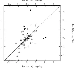
The accuracy plot for the variogram model calcu-lated in equation 1 is given in Figure 8. Dots indicate outliers being outside the 99% confidence limit of a normal distribution.

References

Analytical Methods Committee 1995. Uncertainty of measure-ment: implications of its use in analytical science. Analyst 120:2303–2308.

Armstrong, M. 1998. Basic linear geostatistics. Springer, Ber-lin 146.

Barabas, N., P. Goovaerts, and P. Adriaens. 2001. Geostatisti-cal assessment and validation of uncertainty for three-di-mensional dioxin data from sediments in an estuarine river.

Environmental Science and Technology 35:3294 –3301.

Bouma, J. 2002. Land quality indicators of sustainable land management across scales. Agriculture, Ecosystems and

Envi-ronment 88(2):129 –136.

Bouma, J., H. W. G. Booltink, and A. Stein. 1996. Reliability of soil data and risk assessment of data applications. Soil Science

Society of America Special Publication 47:677.

Cressie, N. A. C. 1993. Statistics for spatial data. John Wiley, New York 900.

Desaules, A., J. Sprengart, G. Wagner, H. Muntau, and S. Theocharopoulos. 2001. Description of the test area and

reference sampling at Dornach. The Science of the Total

En-vironment 264:17–26.

Deutsch, C. V., and A. G. Journel. 1998. GSLIB Geostatistical software library and user’s guide. ., New York 369. Dubois, J.-P., and R. Schulin. 1993. Sampling and analytical

techniques as limiting factors in soil monitoring. Pages 271–273 in R. Schulin, A. Desaules, R. Webster, and B. von Steiger. Eds, Soil monitoring— early detection and survey-ing of soil contamination and degradation. Birkha¨user, Basel.

Fresenius, W., A. Kettrup, and R. W. Scholz. 1995. Gro¨ssenor-dnung Faktor 2: Zur Genauigkeit von Messungen bei Alt-lasten. Altlasten Spektrum 4:217–218.

Geiger G., and R. Schulin (1995) Risikoanalyse, Sanierungs-und U¨ berwachungsvorschla¨ge fu¨r das schwermetall-belastete Gebiet von Dornach. Berichte 2. Volkswirtschafts-departement des Kantons Solothurn, Amt fu¨ r Umwelts-chutz, Solothurn, 79 pp

Geovariances. (1997) Isatis. Geostatistical software. Version 3.1.2. Avon

Goovaerts, P. 1997. Geostatistics for natural resources evalua-tion. Oxford University Press, New York 483.

Goovaerts, P. 2000. Estimation or simulation of soil proper-ties? An optimization problem with conflicting criteria.

Geo-derma 97:165–186.

Goovaerts, P. 2001. Geostatistical modelling of uncertainty in soil science. Geoderma 103:3–26.

Goovaerts, P., and V. Meirvenne. 2001. Delineation of harzard areas and additional sampling strategy in prescence of a location specific threshold. Pages 125–136 in A. Soares, J. Gomez-Hernandez, and J. Froidevaus. Eds, geoENVIII— geostatistics for environmental applications. Kluwer Aca-demic Publishers, Dordrecht.

Goovaerts, P., R. Webster, and J.-P. Dubois. 1997. Assessing the risk of soil contamination in the Swiss Jura using indi-cator geostatistics. Environmental and Ecological Statistics 4:31– 48.

Gotway, C. A. 1994. The use of conditional simulation in nuclear-waste-site performance assessment. Technometrics 36:129 –140.

Gotway C. A., B. M. Rutherford (1993) Stochastic simulation for imaging spatial uncertainty: comparison and evaluation of available algorithms. Pages 1–21 in Geostatistical

Simula-tions. Fontainebleau, France.

Grunewald, K. 1997. Grossra¨umige Bodenkontamination. Springer, Berlin 250.

Gysi C., S., Gupta W., Ja¨ggi J. -A. Neyroud (1991) Wegleitung zur Beurteilung der Bodenfruchtbarkeit. Eidgeno¨ssische Forschungsanstalt fu¨ r Agrikulturchemie und Umwelthy-giene, Liebefeld-Bern, 89 pp.

Hendriks, C., R. Obernosterer, D. Muller, S. Kytzia, P. Baccini, and P. H. Brunner. 2000. Material flow analysis. Case stud-ies on the city of Vienna and the Swiss lowlands. Local

Environment 5:311–328.

Hesske, S., M. Scha¨rli, O. Tietje, and R. W. Scholz. 1998. Zum Umgang mit Schwermetallen im Boden: Falldossier Dor-nach. Pabst Science Publishers, Lengerich 145.

Figure 8. The accuracy plot for the variogram model calcu-lated in equation 1. Dots indicate outliers being outside the 99% confidence limit of a normal distribution.

Journel, A. G. 1974. Geostatistics for Conditional Simulation of Ore Bodies. Economic Geology 69:673– 68.

Journel A. G. (1989) Fundamentals of geostatistics in five lessons. American Geophysical Union, Washington, DC, 40 pp.

Journel, A. G., and C. J. Huijbregts. 1978. Mining geostatistics. Academic Press, London 599.

Keller, A., B. von Steiger, S. E. A. T. M. van der Zee, and R. Schulin. 2001. A stochastic empirical model for regional heavy-metal balances in agroecosystems. Journal of

Environ-mental Quality 30:1976 –1989.

Keller, A., K. Abbaspour, and R. Schulin. 2002. Assessment of uncertainty and risk in modeling regional heavy metal ac-cumulation in agricultural soils. Journal of Environmental

Quality 31:175–187.

Limpert, E., W. A. Stahel, and M. Abbt. 2001. Log-normal distributions across the sciences: keys and clues. Bioscience 51:341–352.

Matheron, G. 1963. Principles of geostatistics. Economic Geology 58:1246 –1266.

Meuli, R., O. Atteia, J. P. Dubois, R. Schulin, B. von Steiger, J.-C. Vedy, R. Webster (1994). Geostatistical interpolation in regional mapping of soil contamination by heavy metals. A case study comparing two rural regions in Switzerland. In FOEFL (ed.), Regional soil contamination surveying,

environ-mental documentation., Federal Office of Environment,

For-ests and Landscape, Bern, pp 43.

Meuli R. G. (1997). Geostatistical analysis of regional soil contamination by heavy metals. Dissertation ETH No. 12121, Swiss Federal Institute of Technology Zu¨ rich, 191 pp.

Mowrer, H. T. 2000. Uncertainty in natural resource decision support systems: sources, interpretations, and importance.

Computers and Electronics in Agriculture 27:139 –154.

Muntau, H., A. Rehnert, A. Desaules, G. Wagner, S. Theocha-ropoulous, and P. Quevauviller. 2001. Analytical aspects of the CEEM soil project. The Science of the Total Environment 264:27– 49.

Pan, G. 1997. Conditional simulation as a tool for measuring uncertainties in petroleum exploration. Nonrenewable

Re-sources 6:285–293.

Papritz, A., and R. A. Moyeed. 1999. Linear and non-linear kriging methods: tools for monitoring soil pollution. Pages 304 –340 in V. Barnett, A. Stein, and K. Feridun Turkman. Eds, Statistics for environment 4: pollution assessment and control. 4. John Wiley & Sons, London.

Prato, T. 2000. Multiple attribute evaluation of landscape management. Journal of Environmental Management

60:325–337.

Ramsey, M. 1998. Sampling as a source of measurement un-certainty: techniques for quantification and comparison with analytical sources. Journal of Analytical Atomic

Spectrom-etry 13:97–104.

Ramsey, M. H, and A. Argayraki. 1997. Estimation of measure-ment uncertainty from field sampling: implications for the classification of contaminated land. The Science of the Total

Environment 198:243–257.

Ramsey M. H., A. Argyraki, S. Squire (1998) Measurement

uncertainty arising from sampling contaminated land: a tool for evaluating fitness-for-purpose. In ConSoil’98. Edin-burgh, UK, pp 221–240

Roe, E., and M. van Eeten. 2001. Threshold-based resource management; a framework for comprehensive ecosystem management. Environmental Management 27:195–214. Saito H. and P. Goovaerts (2000).⬙Geostatistical Interpolation

of Positively Skewed and Censored Data in a Dioxin-Con-taminated Site⬙. Environmental Science and Technology 34:4228 – 4235.

Saito H., and P. Goovaerts (2001).⬙Accounting for source location and transport direction into geostatistical predic-tion of contaminants⬙. Environmental Science and Technology 35:4823– 4829.

Schulin, R., R. Webster, and R. Meuli. 1994. Technical note on objectives, sampling design, and procedures in assessing regional soil pollution and the application of geostatistical analysis in such surveys. Federal Office of Environment, Forests and Landscape, Bern 31.

Schweizerische Meteorologische Anstalt (1982–91). Klimaat-las der Schweiz. AtKlimaat-las climatologique de la Suisse. Atlante climatologico della Suizzera. Lfg. 1-4, Verlag des Bundesa-mtes fu¨ r Landestopographie, Wabern, Bern.

Stahel, W. A. 2000. Statistische Datenanalyse. Vieweg,

Braun-schweig/Wiesbaden .:380.

Theocharopoulos, S. P., G. Wagner, J. Sprengart, M. -E. Mohr, A. Desaules, H. Muntau, M. Christou, and P. Quevauviller. 2001. European soil sampling guidelines for soil pollution studies. The Science of the Total Environment 264:51– 62. Thompson, M. 1995. Uncertainty in an uncertain world.

An-alyst 120:117–118.

Thompson, M., and T. Fearn. 1990. What excatly is fitness for purpose in analytical measurement?. Analyst 121:273–278. Tietje O. (1993) Ra¨umliche Varibilita¨t bei der Modellierung

der Bodenwasserbewegung in der ungesa¨ttigten Zone. PhD. thesis. Technische Universita¨t Braunschweig, 117 pp. Tiktak, A., A. Leijnse, and H. Vissenberg. 1999. Uncertainty in

a regional-scale assessment of cadmium accumulation in the Netherlands. Journal of Environmental Quality

28:461– 470.

Tuchschmid M. P. (1995) Quantifizierung und Regional-isierung von Schwermetall- und Flourgehalten bodenbil-dender Gesteine der Schweiz. Bundesamt fu¨ r Umwelt, Wald und Landschaft, Umwelt-Materialien Nr. 32, Bern, 130 pp. Van Meirvenne, M. 2001. Evaluating the probability of exceed-ing a site-specific soil cadmium contamination threshold.

Geoderma 102:75–100.

VBBo (1998) Verordnung u¨ ber Belastungen des Bodens vom 1. Juli 1998 (Swiss Ordinance on the Pollution of Soils). SR 814.12, Bern.

von Holst, C. 1997. Beurteilung der Qualita¨t von Analysen-daten mit statistischen Methoden unter Beru¨ cksichtigung der Probennahme und der analytischen Bestimmung. Pages 139 –145 in S. Schulte-Hostede, R. Freitag, A. Kettrup, and W. Fresenius. Eds, Altlasten-Bewertung, Datenanaylse und Gefahrenbewertung. ecomed, Landsberg.

1996. Mapping heavy metals in polluted soil by disjunctive kriging. Environmental Pollution 94:205–215.

Wa¨chter, H. 1997. Mo¨glichkeiten und Grenzen der Routin-eanalytik bei der U¨ berpru¨fung von Schwellenwerten – Er-fahrungen aus der Praxis eines Umweltlabors. Pages 30 – 43

in S. Schulte-Hostede, R. Freitag, A. Kettrup, and W.

Frese-nius. Eds, Altlasten-Bewertung, Datenanaylse und Gefahr-enbewertung. ecomed, Landsberg.

Wagner, G., M. -E. Mohr, J. Sprengart, A. Desaules, H. Mun-tau, S. Theocharopoulus, and P. Quevauviller. 2001a. Ob-jectives, concept and design of the CEEM soil project. The

Science of the Total Environment 254:3–15.

Wagner, G., P. Lischer, H. Theocharopoulos, H. Muntau, A. Desaules, and P. Quevauviller. 2001b. Quantitative evalua-tion of the CEEM soil sampling intercomparison. The Science

of the Total Environment 264:73–101.

Webster, R. 2000. Is soil variation random?. Geoderma 97:149 –163.

Webster, R., and M. A. Oliver. 2001. Geostatistics for Environ-mental Scientists. John Wiley & Sons, Chichester 270. Wirz E., and D. Winisto¨rfer (1987) Bericht u¨ ber

Metallge-halte in Boden- und Vegetationsproben aus dem Raum Dornach. Kantonales Laboratorium Solothurn, So-lothurn, 49 pp.