HAL Id: hal-00721374
https://hal.archives-ouvertes.fr/hal-00721374
Submitted on 27 Jul 2012
HAL is a multi-disciplinary open access
archive for the deposit and dissemination of
sci-entific research documents, whether they are
pub-lished or not. The documents may come from
teaching and research institutions in France or
abroad, or from public or private research centers.
L’archive ouverte pluridisciplinaire HAL, est
destinée au dépôt et à la diffusion de documents
scientifiques de niveau recherche, publiés ou non,
émanant des établissements d’enseignement et de
recherche français ou étrangers, des laboratoires
publics ou privés.
Numerical modeling in quantitative ultrasonic
tomography of standing trees
Andrés Arciniegas, Loïc Brancheriau, Philippe Gallet, Philippe Lasaygues
To cite this version:
Andrés Arciniegas, Loïc Brancheriau, Philippe Gallet, Philippe Lasaygues. Numerical modeling in
quantitative ultrasonic tomography of standing trees. Acoustics 2012, Apr 2012, Nantes, France.
pp.1-5. �hal-00721374�
The aim of this project is to develop an ultrasonic device for parametric imaging of standing trees. The device is designed to perform both transmission and reflection measurements that can be therefore used for quantitative tomographic imaging. It allows various automatic acquisitions, since the angular position of the transducers could be adjusted. This makes possible to scan the wave propagation occurring in all directions inside the medium. The associated electronic set-up allows mainly measuring the slowness (and therefore the velocity) and the attenuation of the ultrasonic waves. Tomograms were computed by fast algebraic algorithms: (1) using the filtered backprojection algorithm with fan beam geometry, (2) using a new algorithm that we are developing based on a "layer-stripping" method. Our first numerical results on an academic and realistic phantom of tree are presented in this paper.
1
Introduction
The upward-growth structures on the standing trees are changing fast in order to compete for environmental strength and the natural weather forces, and obviously relatively to the age. These changes result in complex mechanical variations, and the physical properties result of gradual transition from juvenile to mature stage into the tree. In addition to naturally occurring material property variations, abnormal diseases con-tent also varies from the pith to the bark. Anyway, healthy trees can present mechanical weaknesses, and therefore be dangerous in urban environments. Studies have demonstrated the effectiveness of acoustics in detecting/imaging trees’ de-cay. The main commercial acoustic devices for tree assess-ment are essentially based on methods using low frequency acoustic waves. Three tools are "PICUS R Sonic Tomograph"
(Germany) [1], the "ARBOTOM R" [2] (Germany), and the
"FAKOPP" [3] (Hungary). They use an impulse hammer to excite the trunk and measure the acceleration on circumferen-tial points (accelerometer) with a limited number of sensors. These methods give average values recorded along the acous-tic pathway, but they are not always suitable to access 2D resolution (about few centimeters for defect size).
During the last decade, ultrasonic tomography made con-siderable progress in medical and industrial domain. With the evolution of the electro-acoustical technology new devices for image acquisition have appeared. The main aim of our project is to develop a mechanical ultrasonic imaging device for standing trees (ARB’UST) using two transducers (from 50 to 90 kHz), that could be transportable and used in an in situcondition. With ARB’UST, data is collected sending energy through the tree as many different angles as used to compute an image of the changes of a physical quantity in a slice. The ultrasonic waves cross from the emitter to the receiver at appropriate locations around the tree. These loca-tions are chosen so that as many rays pass through as much of the object as possible. The parameter measured is the time-of-flight (travel time) of the ultrasonic wave between the emitter and the receiver. The final ultrasonic tomogram represents the slowness (the velocity) distribution (related to the axial and lateral resolution of the transducers) in a thin cross-section of the tree (related to the elevational resolution of the transducers).
In ultrasonic tomography different approaches have al-ready been proposed in literature [4, 5, 6]. There are two major classes of reconstruction techniques. One class is based on the projection-slice theorem such as the filtered backpro-jection method (FBP). This method is fast and the data must be acquired on spaced sets of straight ray paths (projections). The main actual challenge in tree imaging is the choice of the effective method to inverse the scattered data, and the first step in this work is to test two tomographic inversion meth-ods. This paper focus in an approach by numerical simulation
of the reconstructions of cylindrical homogeneous isotropic medium with defects.
2
Materials and methods
In this paper a comprehensive study is conducted on the re-construction capability of travel time tomography method for a ring transducer scanner using computed-simulated data for a numerical tree phantom. The scheme to simulate ultrasonic-wave propagation through the phantom depends of the experi-mental set-up and assumptions.
From the mechanical point of view, ARB’UST device was designed to perform sectorial scanning such as fan beam or transmission mode. The general architecture of the system is that of an ultrasound tomographic scanner. An aluminum ring holds two 50 kHz - transducers allowing the bi-static 2D-survey around the trunk [7].
The numerical simulation can be used to study the ac-curacy of different travel time tomography for different tree phantoms (shapes and physical properties mimics). Numeri-cal tree phantoms are placed inside a ring where transducers are positioned at the boundaries at regular angular spacing lo-cations, from 0oto 360o. A 120ocircular sector is not scanned
due to positions where the receiver cannot be experimentally placed (Figure 1). A typical angular step of 4o leads to 61 points per projection. For a complete scan, the total number of acquisitions is therefore 5490. For one projection, the emitter remains in its position while the receiver moves around the ring (Figure 1).
Figure 1: The principle of acquisition
For this purpose, pure compression ultrasonic wave were transmitted in the sample, and no shear waves were taken into account. The medium was supposed homogeneous and isotropic. The wave velocities were independent of frequency. The ultrasonic wave attenuation would be neglected. Only the propagation path phenomena were considered, and the wave delays studied. The numerical tree phantom was then repre-sented by the ultrasonic slowness distribution, and each pixel had a constant value of slowness of the ultrasonic wave. The implementation of the phantom, algorithms and simulations was made in MATLAB R.
2.1
Mimicking phantom of tree
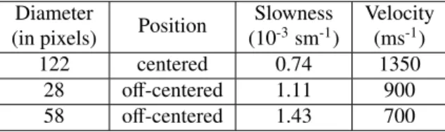
Simulations can be easily performed for a large number of well-controlled mimicking phantoms of tree, and can help to understand the features of wavefields acquired by transducers. The simulation can then be used to study the accuracy of travel time tomography for different sizes and shapes of phantom. In this paper, it is proposed to apply this method for a phantom having two main perturbation sizes and shapes inside the host medium and including a small defect. The numerical phantom is a cylindrical homogeneous isotropic object, with cylindrical homogeneous isotropic pertubations (Figure 2). Each small point at the boundaries of the object represent an angular position where the emitter is going to be placed. Table 1 shows the parameters used to construct the phantom.
Figure 2: Numerical phantom. o : Positions where the sensors are going to be experimentally placed.
Table 1: Parameters of the phantom Diameter
Position Slowness Velocity (in pixels) (10-3sm-1) (ms-1)
122 centered 0.74 1350 28 off-centered 1.11 900 58 off-centered 1.43 700
2.2
Forward problem
To test the reconstruction algorithms, it was carried out a numerical implementation of the experimental protocol (ac-quisition sequences). Equation 1 is known as the Radon transform of a function f(x, y).
Pθ(τ)= Z
(θ,τ) line
f(x, y)ds (1) In the reality, the function f represents the physical param-eter to be measured. For a fan beam geometry, an independent measurement, or point of projection, is defined as the ray in-tegral (along the line τ) as is given by Pθ(τ) for a constant observation angle θ [4]. A projection is therefore the collec-tion of the ray integrals measured along the fan.
Travel time t between an emitter n and a receiver m is represented by a line integral of the slowness p along the ray pathΓ [8], as shown in Eq. 2.
t(n, m)= Z
Γ(n,m)
p(x, y)dΓ (2)
The discrete forward problem for an independent travel time measurement is then approximated by a weighted sum-mation for N pixels crossed by a given ray path (Eq. 3).
t(n, m)= N X q=1 Γ(n,m) pqdq (3)
The distance D for a given path is assumed as a multiple of constant discrete step dq(pixel), thus D= Ndq. Dividing
each side of Eq. 3 by D, the numerical implementation of Radon transform for the slowness P(n,m) is then:
P(n, m)= 1 N
X
Γ(n,m)
p(x, y) (4)
2.3
Reconstruction by the filtered
backprojec-tion method (reference method)
Let us consider a mesh of pixels. To find the value of the slowness at any point of the object, it is assigned the value of the projection at any pixel placed in the path that it covers, and then adding all contributions from all projections. This principle is called backprojection. This method, however, leads to biased values and it is necessary to correct each projection by a specific filtering. The filtered backprojection consists therefore initially to filter each projection using a ramp filter (often combined with a low pass filter to avoid noise amplification), and then to project back the filtered projections for the different observation angles [4].
2.4
Reconstruction by the Layer Stripping
based method
In this paper, it is proposed an application of a new in-version algorithm based on a "Layer Stripping" method [9]. This procedure is an iterative approach, for transmission mea-surements in fan-beam mode, where ray paths are analyzed as if the object was discretized by concentric layers. The tomographic reconstruction consists of the local estimation of slowness of an identified concentric layer and to correct it with respect to the values of slowness that were already calculated in the previous layers. Analysis towards the center leads the evolution of the reconstruction. This multi-layer approach is adapted to the tree because their circumferential cross section, from internal to external, can be associated to a 2D annular structure.
2.4.1 Discretization
The number of layers depends on the number of transduc-ers. N (pair) transducers are distributed uniformly around the object every 360o/ N (angular step). Equation 5 shows that the value of the radius of a layer is determined by:
d(k)= minM∈D|C − M| ; ∀ 1 ≤ k ≤ N/2; k ∈ N (5)
Where:
d(k): the distance from the layer k towards the center (radius of the layer). Thus the mesh is composed by N/2 layers. C: is the center of the object.
D: the straight ray linking transducers E1Ek+1
2.4.2 Algorithm
Let Eq. 6 describe the slowness for a simple backpro-jection process. Γ is the straight ray connecting the emitter E(n) to the receiver E(m).Ω(i, j) the set of straight rays that intersect a pixel at (i,j), where i and j are the index of the resulting image by the reconstruction1. |Ω| is the number of
straight rays of the set.
p(i, j)= 1 |Ω|
X
Ω(i, j)
P(n, m) (6)
From the foward problem, and assuming the existance of nested layers, Eq. 4 could be explained by Eq. 7 .
NP(n, m)= X layer k−1 pk−1(i, j)+ X layer k pk(i, j) (7)
A generalization of Eq. 4 leads to the slowness P of a layer. Slowness at a layer k-1 and k is then estimated as shown in Eq. 8 and Eq. 9.
X layer k−1 pk−1(i, j)= Nk−1Pk−1 (8) X layer k pk(i, j)= NkPk (9)
where Nk−1and Nkare the number of pixels at layers k-1
and k respectively.
Replacing Eq. 9 in Eq. 7, the correction formula for P(n,m) is then calculated as follows:
NP(n, m)= X layer k−1 pk−1(i, j)+ NkPk (10) ˆ Pk(n, m)= NP(n, m) − X layer k−1 pk−1(i, j) Nk (11) where ˆPk(n, m) is the corrected value of the
backprojec-tion. Recursive application of Eq. 11 into Eq. 6 leads to the reconstruction. For each iteration, the upper part of Eq. 11 should be positive to guarantee the convergence to a solution.
3
Results
3.1
Forward Problem
Figure 3 shows the ultrasonic sinogram formed by 90 ob-servation angles (angular step of 4o). Ray theory was applied
without taking into account the attenuation in the different media. The color of each pixel corresponds to the slowness measured between two elementary sensors. Each line of the matrix corresponds to a projection.
3.2
Reconstruction and processing – Inverse
Problem
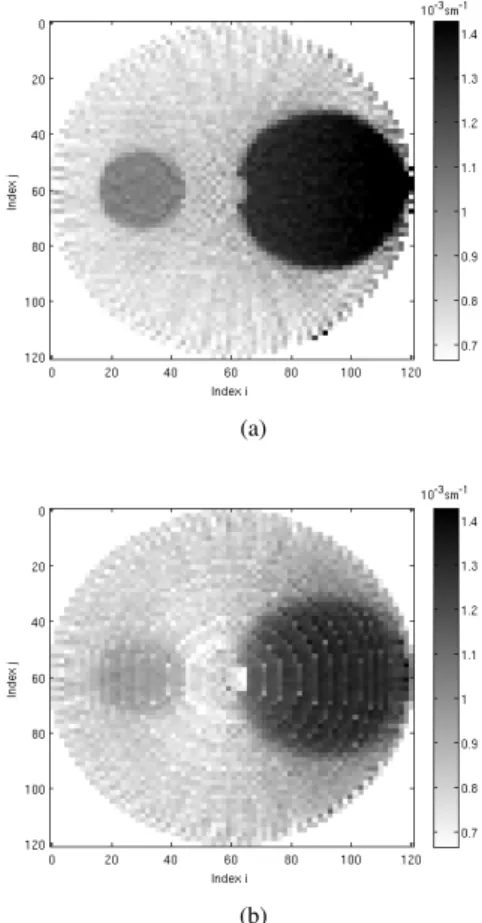
Figure 4 shows the reconstructed object associated to each inversion algorithm. The reconstructed objects are smaller with respect to the original phantom. The theoretical number
1Size of the phantom and reconstructed image are different.
of pixels that allow to reconstruct the scanned area with 90 emitter positions is 4005 [8]. The optimal size of the asso-ciated image is then 72x72 pixels. Note that the quality of the reconstructions obtained in Figure 4 is partly due to the fact that the forward problem and inverse problem involve the same approximate theory of straight ray propagation.
Figure 3: Simulated ultrasonic sinogram.
(a)
(b)
Figure 4: Reconstruction by: a) Filtered backprojection; b) Layer Stripping
Figure 5 shows the uncertainty of the linear model Y=aX+b that compares the reconstructed measured slowness (X= pro-jections of the reconstructed image (depend of the algorithm)) with respect to initial measured values (Y= projections of the phantom). The analysis were carried out with a confidence interval of 95% and each test was realized for the reconstruc-tion for a given number of sensors. Figure 6 shows the mean of absolute deviations (mean deviation per pixel) between the reconstructed image and the phantom. The analysis was carried out by linear interpolation of the reconstructed image to the size of the phantom and comparing the deviation pixel
per pixel. When noise is not taken into account, both figures show that when this range of sensors (24 - 96) is used, the un-certainties decrease. Because the observations for further than 96 sensors were not tested, conclusion about the asymptotic behavior was not established. Reconstructions by the Layer Stripping algorithm are less performing than those carried out by the inversion by FBP. For a scan with 90 sensors, the respective uncertainties of the linear model were 7.2% (FBP) and 12.6% (LS). The mean deviations per pixel were about 0.079x10⁻³sm-1(FBP) and 0.124x10⁻³sm-1(LS); to be
com-pared with the mean pixel value of 0.92x10⁻³sm-1inside the
scanned area of the phantom. For each one of these figures the slopes of each pair of curves are similar. Both inversion methods present similar behavior according to the number of sensors used for a given scan.
Figure 5: Linear model uncertainty according to the number of sensors for: o Filtered backprojection, * Layer Stripping
Figure 6: Mean deviation per pixel according to the number of sensors for: o Filtered backprojection, * Layer Stripping
Figures 7 and 8 show respectively the evolution of the linear model uncertainty and of the mean deviation per pixel when Gaussian noise is present for the same scan with 90 sensors. As noise increases, the uncertainties do it as well, but the behavior for the two inversion methods is different. The slopes of the curves of the uncertainties for the reconstructions by FBP are more sensitive to noise than for those by Layer Stripping. From about 20% of noise, the mean deviation per pixel for Layer Stripping is lower than for the FBP. For example at 30% of noise, linear model uncertainties are 15.7% (FBP) and 16.8% (LS), and are related to 0.209x10⁻³sm-1and 0.173x10⁻³sm-1deviation per pixel respectively.
Figure 7: Linear model uncertainty according to the percentage of noise considered for: o Filtered backprojection,
* Layer Stripping
Figure 8: Mean deviation per pixel according to the percentage of noise considered for: o Filtered backprojection,
* Layer Stripping
4
Conclusion
A new inversion algorithm has been presented as well as first numerical results. The tests consisted to simulate travel time tomography with the aim to compare the inversion of numerical data by Layer Stripping in relation to the inversion by Filtered Backprojection (reference method). These simu-lations depended of the experimental set-up of the ultrasonic tomograph and assumptions for the numerical phantom. For this first approach the phantom was assumed to be a cylindri-cal homogeneous isotropic medium with defects. Ray theory was applied without taking into account the attenuation. Quan-titative analysis included the comparison of the uncertainties of the projections and slowness values of the reconstructed images with respect to the phantom. The first analysis showed that if noise is not taken into account, as more sensors are used for a scan, uncertainties decrease. Both inversion algorithms presented similar behavior according to the number of sensors. A general conclusion about this behavior was not established because tests were developed for a specific range of number of sensors. The results showed that if noise is not taken into account, uncertainties for Layer Stripping are greater than for FBP. The second analysis showed that, for a given scan, as noise increases, uncertainties do it as well, however the reconstructions by the FBP became more sensitive than those by Layer Stripping.
These results are the first step for further research in nu-merical modeling and experimental testing with samples of trees. In this paper it was underlined that the approach by Layer Stripping could be adapted to trees because it can be
associated to their 2D annular structure. A next step in numer-ical modeling should be the choice of a phantom with a con-centric layer geometry. In relation to the inversion algorithms, because the actual challenge in tree imaging is the choice of the effective method to inverse scattered data, several recon-struction methods, from analytical to algebraic, should be also tested. Experimental tests using our tomographic device are also planned to be carried out.
Acknowledgments
This study was based on the research supported by the French National Research Agency (BioGMID - Biological Growth Medium Integrity Diagnoses using bi-modality tomo-graphies) under the Grant no183692 to USAR-CNRS.
References
[1] S. Rust, “A new tomographic device for the nondestruc-tive testing of trees,” in 12th Int. Symposium on NDT of Wood, (Sopron, Hungary), pp. 233–237, University of West Hungary, Hungary, 2000.
[2] F. Rinn, “Holzanatomische grundlagen der schall-tomographie an baumen,” Neue Landschaft, vol. 7, pp. 44– 47, 2004.
[3] F. Divos and P. Divos, “Resolution of stress wave based acoustic tomography,” in 14th Int. Symposium on NDT of Wood, (Hannover, Germany), pp. 309–314, Shaker Verlag, Aachen, Germany, 2005.
[4] A. C. Kak and M. Slaney, Principles of Computerized Tomographic Imaging. Society of Industrial and Applied Mathematics, 2001.
[5] P. Grangeat, La tomographie : fondements mathéma-tiques, imagerie microscopique et imagerie industrielle. Paris, France: Lavoisier, 2002.
[6] J.-P. Lefebvre, P. Lasaygues, and S. Mensah, Materials and Acoustics Handbook, ch. Acoustic Tomography, Ul-trasonic Tomography. London, UK: ISTE, 2010. [7] L. Brancheriau, P. Gallet, and P. Lasaygues, “Ultrasonic
imaging defects in standing trees – development of an automatic device for plantations,” in 17th Int. Symposium on NDT of Wood, vol. 1, (Sopron, Hungary), pp. 93–100, University of West Hungary, Hungary, 2011.
[8] L. V. Socco, L. Sambuelli, R. Martinis, E. Comino, and G. Nicolotti, “Feasibility of ultrasonic tomography for non-destructive testing of decay on living trees,” Research in Nondestructive Evaluation, 2004.
[9] E. Franceschini, Tomographie ultrasonore dédiée à la détection du cancer du sein. PhD thesis, Université de Provence - Aix-Marseille I, 2006.