A distance measure between plant architectures

HAL Id: hal-00827474

https://hal.inria.fr/hal-00827474

HAL is a multi-disciplinary open access archive for the deposit and dissemination of sci-entific research documents, whether they are pub-lished or not. The documents may come from teaching and research institutions in France or abroad, or from public or private research centers.

L’archive ouverte pluridisciplinaire HAL, est destinée au dépôt et à la diffusion de documents scientifiques de niveau recherche, publiés ou non, émanant des établissements d’enseignement et de recherche français ou étrangers, des laboratoires publics ou privés.

est Science, Springer Nature (since 2011)/EDP Science (until 2010), 2000, 57 (5/6), pp.445-461. �10.1051/forest:2000134�. �hal-00827474�

Original article

A distance measure between plant architectures

Pascal Ferraro

_{and Christophe Godin}

Plant Modelling Program – CIRAD, Programme de modélisation des plantes, TA/40E, 34398 Montpellier Cedex 5, France (Received 1 February 1999; accepted 18 February 2000)

Abstract – In many biological fields (e.g. horticulture, forestry, botany), a need exists to quantify different types of variability within

a set of plants. In this paper, we propose a method to compare plant individuals based on a detailed comparison of their architectures. The core of the method relies on an adaptation of an algorithm for comparing rooted tree graphs, recently proposed by Zhang in theo-retical computer science. Using this algorithm a distance between two plants is defined as the cost of transforming one into the other (using basic “edit operations”). We illustrate this method in three application fields and then compare it with other methods for quan-tifying plant similarity.

topological structure of plants / plant comparison / analytical method

Résumé – Définition d’une distance entre architectures de plantes. Dans de nombreux domaines de la biologie (arboriculture,

sylviculture, botanique), il est nécessaire d’étudier différents types de variabilité au sein d’une population de plantes. Nous propo-sons, dans ce papier, une méthode de comparaison des plantes basée sur une comparaison détaillée de leur architecture. Cette métho-de est une adaptation d’un algorithme métho-de comparaison d’arborescences, proposé récemment par Zhang en informatique théorique. Cet algorithme nous permet de définir une distance entre deux plantes comme le coût de la transformation de l’une en l’autre (à l’aide d’opérations élémentaires d’édition). Cette méthode est illustrée dans trois domaines d’application et elle est comparée à d’autres méthodes de quantification de la ressemblance entre plantes.

structure topologique des plantes / comparaison des plantes / méthode analytique

1. INTRODUCTION

The increasingly important role played by plant archi-tecture in the structure/function modeling of plants gen-erates a need for new investigational tools. Generic tools have already been developed to visualize plant architec-ture in 3-dimensions [4, 30], to model the growth of plant architecture, e.g. [5, 20, 21, 25], to measure plant architecture [9, 14, 33], and to explore and to analyze the plant [10]. This paper introduces a new tool for the com-parison of plant architectures.

To compare two plants, a first approach consists of summarizing each individual by a small number of

syn-thetic and global variables (e.g. fruit production, crown size, etc.). The similarity of two individuals is then reduced to the similarity between these synthetic vari-ables. In forestry for instance, wood production and quality are usually assessed by measuring variables such as stem diameter, crown volume, branching density, etc. Comparing different wood qualities thus amounts to comparing these global variables. This defines global comparison methods in which the topological organiza-tion of plant entities is not taken into account.

On the other hand, domains exist in which plant topo-logical structure plays an important role. In forestry for example, refining wood quality criteria leads foresters to

* Correspondence and reprints

In such cases, the notion of distance between individuals would naturally take into account the topological and spatial organization of plant entities. This defines analyt-ical comparison methods [26] which are based on a piece-by-piece comparison of plants.

In most applications, descriptions of plant architecture usually rely on a tree graph representation of topological structures [8]. An algorithm with bounded complexity has recently been proposed in theoretical computer sci-ence to compute a distance between tree graphs [43, 44]. This distance is defined as the minimum cost of the

use of this comparison algorithm is illustrated in three different application contexts.

2. FORMAL REPRESENTATION OF PLANTS AS TREE GRAPHS

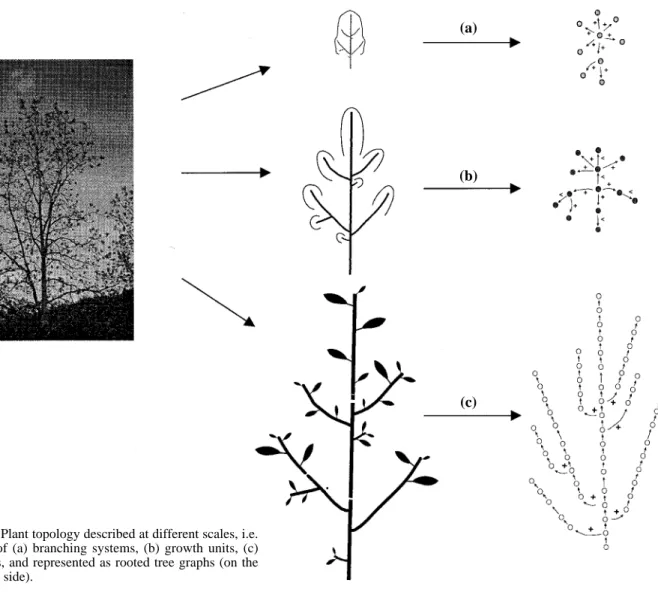
A plant can be considered as a set of botanical entities (e.g. internodes and nodes, growth units, annual shoots) the topological organization of which can be represented by a graph [8] (figure 1). A graph G = {V,E} consists of

Figure 1. Plant topology described at different scales, i.e.

in terms of (a) branching systems, (b) growth units, (c) internodes, and represented as rooted tree graphs (on the right hand side).

(a)

(b)

a set V of vertices and a set of edges E, each edge being represented by an ordered pair of vertices [29]. If (v1, v2)

denotes an edge in E, the vertex v1is called a father of v2

and the vertex v2is called a son of v1[29]. Vertices

rep-resent botanical entities and edges correspond to the physical connections between these entities. Each vertex can be associated with one or several attributes that rep-resent biological characteristics of the entity and consists of either a real number (e.g. entity diameter, length), or a symbol (e.g. entity type). Let α be a labeling function which associates a label from a finite or infinite set

Σ= {a,b,c,...} with each vertex. A distance d, called ele-mentary distance, is supposed to be defined on labels. A distance on vertices of a graph can be defined using the distance on labels: d(v1,v2) = d(α(v1),α( v2)). Let λbe a

unique symbol not in Σ,d is extended by defining quan-tities d(α(v1),λ) and d(λ,α(v2)) so that d is a distance on

Σø {λ}. The distance d(α(v1),λ) between the label of a

vertex v1 and the label λ is denoted by d(v1,λ) by

convention.

In a plant, since each entity is physically attached to at most one parent entity, the topological structure is repre-sented as a rooted tree graph, i.e. a graph in which every vertex except one, called the root, has only one father vertex. The root has no father vertex. In order to identify the different axes on a given plant, two types of edges between entities are distinguished: an entity can either precede (symbol “<”) or bear (symbol “+”) another enti-ty. This form of plant description can now be used to present an analytical method for comparing plants.

3. PLANT COMPARISON METHOD

A considerable amount of work has been performed on comparison algorithms for problems that can be mod-eled as data sequences [35]: in molecular biology [16, 34], in speech or text recognition [23] or in code error correction [39], in plant modeling [11]. In the early sev-enties, Wagner and Fisher [42] presented an algorithm which computes the distance between two strings of characters as the minimum cost sequence of elementary operations needed to transform one string into the other. In order to define a distance between rooted tree graphs, Tai [37], Selkow [32] and Lu [24] proposed a generaliza-tion of the Wagner and Fisher algorithm with applicageneraliza-tion in different fields [27, 28, 32]. All the tree graphs dis-cussed in these papers are ordered, meaning that the sets of sons of any vertex are ordered sets. These algorithms cannot be applied directly to the problem of plant com-parison since tree graphs used to represent plant topolo-gy are unordered [8]. However, recently, Zhang [43, 44] proposed an algorithm in theoretical computer science for computing a distance between unordered rooted tree

graphs based on Lu’s method, by introducing a new hypothesis in the tree-graph transform. This paper briefly describes the main principle of the algorithm and illus-trates several applications to plant comparison.

A distance measure between two trees T1 and T2 is

defined by considering the minimum cost of elementary operations needed to transform T1into T2. Three kinds of

elementary operations, called edit operations [42] are considered: changing one vertex into another (note that this may change labels), deleting (i.e. making the sons of a vertex v become the sons of the father of v and then removing v from T1) or inserting one vertex (i.e. the

symmetric operation on T2) (figure 2a). In order to

trans-form one tree graph into the other, all the vertices of T1

and T2must be affected by at least one edit operation.

A cost function, called local distance, is defined for each edit operation s. The local distance assigns a non-negative real number γ(s) to s:

•γ(s) = d(v1,v2) if s changes the vertex v1into the

ver-tex v2,

•γ(s) = ddel(v1) = d(v1,λ) if s deletes the vertex v1and,

•γ(s) = dins(v2) = d(λ,v2) if s inserts the vertex v2.

Since d is a distance, the following property is always satisfied:

(1) Let S be a sequence of n edit operations (s1, s2, …, sn) which transform one tree graph T1 into another one T2.

The cost γ(S) of a sequence of edit operations is defined by summing up the cost of the edit operations that compose S: . The set of possible edit operation sequences which transform T1into T2is

denot-ed by S. The dissimilarity measure1_D(T

1,T2) from a tree

graph T1to a tree graph T2is then measured as the

mini-mum cost of a sequence in S:

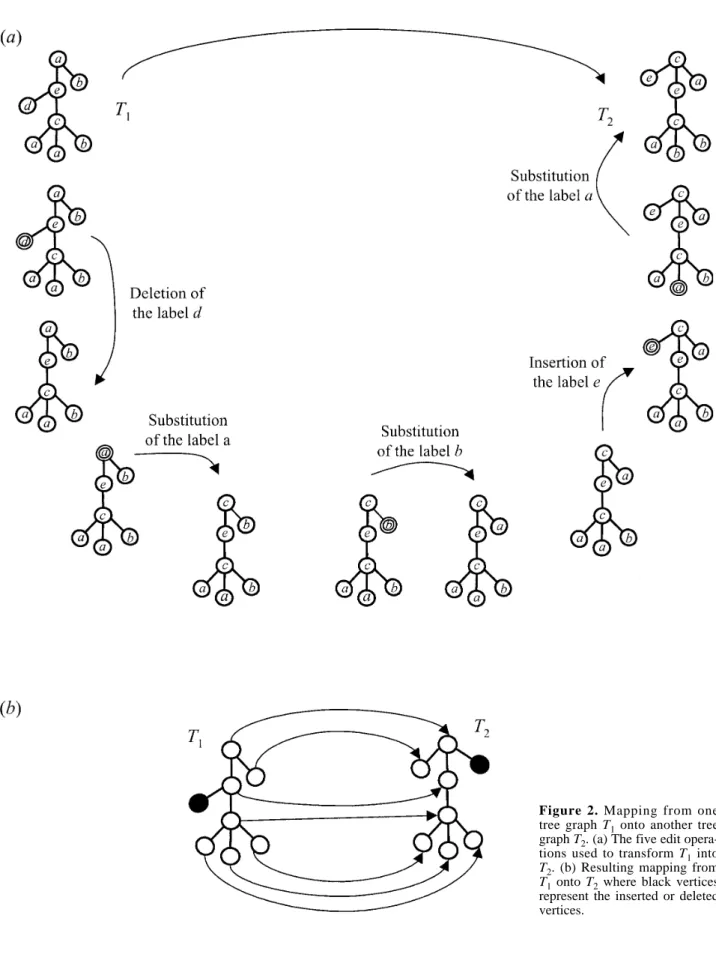
In order to characterize the effect of a sequence of edit operations on a tree graph, Taï [37] introduced a struc-ture called mapping between tree graphs (figure 2b). Based on the notion of trace between Wagner and Fisher strings [42], a mapping is intuitively a description of

D T₁, T2 = min S∈S γ S . γ S =

Σ

1_{A dissimilarity measure d over} Σ_{is a function from} Σ × Σ_to

R+ _{such that for any a,b in Σ d(a,a) = 0, d(a,b) = d(b,a),} d(a,b) = 0 => b = a (symmetry) and such that it does not neces-sarily respect the triangle inequality.

Figure 2. Mapping from one

tree graph T₁onto another tree graph T₂. (a) The five edit opera-tions used to transform T₁into T₂. (b) Resulting mapping from T₁onto T₂where black vertices represent the inserted or deleted vertices.

how a sequence of edit operations transforms T1into T2,

ignoring the order in which the edit operations are applied. A mapping M is a set of ordered pairs (v1, v2) of

vertices from T1×T2(v1and v2are images of one

anoth-er). The set of vertices of T1 (resp. T2) which are

not in a pair of M is denoted by M—1(resp. M

—

2). Note that

M is a set of pairs of vertices while M—1and M

—

2are sets of

vertices. The set of all possible mappings from T1to T2

is denoted by M.

According to the definition of elementary costs, we can assign a cost to each mapping M:

(2)

The relation between a trace and a sequence of edit operations has been made explicit by Wagner and Fisher [42]. This result has been generalized for mappings between ordered tree graphs [37] and unordered tree graphs [43, 45].

Property 1: Given S a sequence of edit operations from T1 to T2, there exists a mapping M from T1 to T2

such that γ(M) ≤ γ(S).

Property 2: For any mapping M from T1 to T2 there

exists a sequence of edit operations such that γ(M) =

γ(S).

Based on these properties it can be shown that the dis-similarity between two tree graphs is measured as the mapping with minimum cost. Indeed, from property 1, we obtain:

Let M*_{be the mapping with minimum cost. From}

prop-erty 2 arises a sequence S*_{of edit operations such that:}

Finally:

and:

(3) This equation shows that the computation of the edit dis-tance between T1 and T2 leads us to solve an

optimiza-tion problem, i.e. finding the mapping with minimum cost over M.

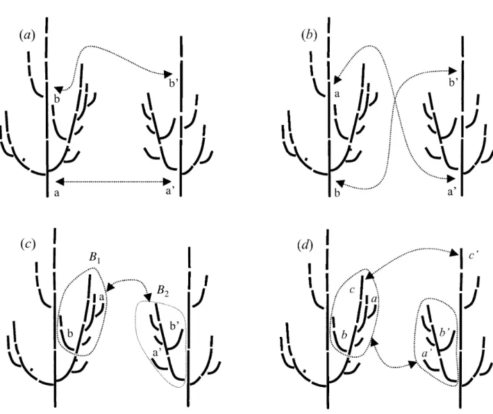
However, when comparing plant architectures, we are not interested in all possible mappings between plants. For example, we do not want to consider mappings that match the trunk of T1with the leaves of T2and the leaves

of T1with the trunk of T2 (figure 3b). Only those

map-pings that preserve certain structural properties will be considered. For example, in the case of sequence align-ment, Wagner’s algorithm preserves the ancestor rela-tionship between elements of the sequence. In a tree graph, a vertex v1is called the ancestor of another vertex

v2if a path2exists from v1to v2. For example, one entity

a, ancestor of an other entity b, can only be mapped onto an entity a’ that is an ancestor of the image b’ of b. This ancestor relationship is also denoted by v1≤v2. Similarly

to sequences, when comparing plant architectures we wish to consider only mappings that preserve the ances-tor relationships (figure 3a).

One of the results from Zhang [45] and Kilpelläinen [17] is that finding the optimal matching function for an unordered tree is an NP-complete problem. This means that there is no reasonable chance of a polynomial-time algorithm solving this optimization problem. Since unordered tree graphs are important in our plant compar-ison applications, it is necessary to change the matching function definition in order to obtain an algorithm that computes the distance between unordered tree graphs in polynomial time.

An intuitive idea to solve this problem was proposed by Tanaka and Tanaka [38] who introduced a distance between ordered trees to preserve structural properties of the tree graphs by the matching functions. Zhang [45] extended the definition from ordered trees to unordered trees. The idea is that two separate sub-trees of one tree graph should be mapped onto two separate sub-trees.

The preservation of sub-trees can be formalized using the notion of least common ancestor. In a tree-graph, the least common ancestor of v1 and v2, denoted by

lca (v1, v2), is a common ancestor of v1 and v2 such that

every common ancestor w of v1 and v2 satisfies

w≤lca (v1, v2). For any vertex pair (v1, v2) of a mapping,

we define a branching system with reference to their least common ancestor (figure 3c). Descendants of the least common ancestor (including the least common ancestor itself) represent the branching system B1. The

images of a1and b2define another branching system B2.

The new constraint implies that: any vertex in branching system B1can only be mapped onto branching system B2.

D T₁, T2 = min S∈S d S = minM∈M d M . min S∈S d S = min M∈M d M γ S * =γ M * = min M∈M γ M ≤ min S∈S γ S . min S∈S γ S ≥ min M∈M γ M . γM =

Σ

Σ

Σ

Mappings that preserve ancestor relationship and tree separation are called valid mappings. A valid mapping M is a set of ordered pairs (v1, v2) of vertices satisfying:

v1∈T1, v2∈T2, and for any pair (v1, v2), (w1, w2), (u1, u2) in M

v1= w1⇔v2= w2 (4)

v1≤w1⇔v2‹ w2 (5)

lca (v1, w1) < u1⇔lca (v2, w2) < u2. (6)

Condition (5) expresses ancestor relationship conserva-tion and condiconserva-tion (6) expresses a conservaconserva-tion of

branching systems. The set of valid matching functions is denoted by Mv. We can now define a dissimilarity measure between T1and T2as:

(7)

Zhang showed that the dissimilarity measure is a dis-tance3_{[43]. According to this definition, Zhang [43, 44]}

D T1, T2 = min

M∈Mvγ M .

3_{This means that D is a dissimilarity measure which respects} the triangle inequality.

Figure 3. Allowed and forbidden matching functions in tree graph comparisons: (a) preservation of ancestor relationship, (b)

non-preservation of ancestor relationship, (c) non-preservation of branching system, (d) non-non-preservation of branching system. This mapping verifies conditions (4) and (5) but not (6).

B

proposed an algorithm with bounded complexity for solving the optimization problem (7) which consists of finding a valid matching function with minimum cost. To improve the analysis of the algorithm output and con-sider new extensions, the computation of matching lists, i.e. the computation of mapped vertices, has been devel-oped in [7].

The algorithm described by Zhang [43, 44] uses a recursive expression for calculating distances between sub-trees of T1 and T2 (detailed in [7]). This algorithm

solves the problem of computing D (T1, T2) in

polynomi-al time. Figure 4 illustrates the computation time in rela-tion with the size of the tree graphs.

4. THE LOCAL COST FUNCTION

As described in [18, 28, 43] and the previous section, if a distance measure is to be determined between sequences or tree graphs based upon edit operations, it is necessary to consider an elementary distance between the components of the sequences or tree graphs. In the case of plant comparison, a local distance (called the local cost function) assigns to each pair of entities (v1, v2) of two plants T1and T2(represented by two tree

graphs), a non-negative real number (called a cost) for deleting v1, for inserting v2, and for changing v1into v2.

There are several possible methods for quantifying the difference between any two plant elements depending on the aim of the application.

A simple cost function used for comparing elementary entities is based on a binary distance called a Levenstein’s distance [22]. In this case, a null cost is

assigned to any changing operation and a cost of one to any insert-delete operation. A local cost defined in this way does not take into account the nature of the entities, so the distance is independent of the entities involved in the operation. A distance based on such a local cost function only involves the topological structure of plants and is called a topological cost.

This binary distance can be refined by using entity attributes such as length, diameter, types, etc., and defin-ing a distance in this space. We will suppose that, for each elementary entity v of T1and T2, precisely n

attrib-utes a1(v), a2(v),…, an(v) are defined which may have symbolic or numerical values. In cases of multiple numerical attributes (n > 1), it is necessary to homoge-nize the attribute dynamics so that they have a compara-ble importance in the definition of the metric. The standardization [15] of data consists of calculating the mean value miof each variable aiand then computing for each plant T a measure of the dispersion of this variable. Traditionally, the standard deviation is used:

(8)

Let us assume that siis not zero (otherwise the variable fi is a constant). The standardized measurements are thus defined by:

(9) For numerical attributes, the elementary distance between two entities (v1, v2) is a metric distance in

n-dimensional space, and in practice this distance is often computed as the Manhattan distance:

(10)

The insert-delete cost can be defined in several ways, provided that equation (1) is satisfied. For example, the insert-delete cost may be chosen to be proportional to the sum of the absolute values of the attributes:

(11) In order to ensure that such a local cost satisfies equation (1), µmust be a real number greater than or equal to 1.0. With such a local distance, the insert-delete cost for each entity is directly dependent upon its nature. Another way to define the insert-delete cost is to render it proportional

d_ins v₁ =µ

Σ

Σ

Σ

Σ

Figure 4. Computation time according to the size of the tree

In order to ensure that such a local cost satisfies equation (1), µmust be a real number strictly greater than 0.5 [7]. Both the insert and delete costs are the most widely used in real and theoretical applications of this method [18].

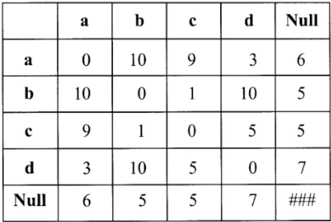
Only a finite number of symbols are available for symbolic attributes. The distance between entities is defined as the distance between the different symbols. In practice the user must construct a cost matrix between these symbols. In figure 5, T1and T2are two theoretical

plants. A symbolic attribute, called a label, taken from {a,b,c,d} is attached to each entity. Table I indicates the heuristic costs used when comparing these labels. If an entity with a given label is inserted or deleted, the assigned cost is shown in the Null column. The changing cost between two elementary entities relies on the com-parison of their labels which is indicated in the corre-sponding cell. In our example, the cost of comparing entity 1 and entity 2 of type a and b respectively, is 10. Thus, plants T1and T2are considered different while in a

topological sense they are identical. With such local costs, the distance between the plants not only takes into account the topological structure of plants but also other architectural information.

Both types of attributes can be mixed within an appro-priate local distance. Let f1, f2,…, fk, be k numerical attribute functions and let fk+1, fk+2,…, fn be n symbolic attribute functions. According to the previous discussion, n cost matrices must be constructed that define, for each symbolic attribute, the distance between symbols. Thus, for each pair of entities (v1, v2) of T1and T2and for each

symbolic attribute fi, there exists a cost ci(v1, v2) for

changing the symbol fi(v1) into fi(v2). In the most general

form, a local distance is expressed as follows:

(13) The local cost function and the insert-delete cost are cho-sen depending on the application. The effect of this choice is discussed in the next section.

5. EFFECT OF COMPARISON PARAMETERS

The distance between plants depends on two main parameters: the topological structure of the plants and the local distance between entities. The effect of both parameters is analyzed hereafter using several sets of theoretical plants represented in figures 6 and 7. In each set of plants (S1), (S2), (S3) and (S4), each pair of plants

was compared by the algorithm using an appropriate local distance. A matrix of the distances between plants was thus obtained and these matrices were studied and analyzed depending on the application.

5.1 Effect of topological structure

Two topological structures may be different because of two major factors: their number of entities and the

d v₁, v2 =

Σ

Σ

Figure 5. Comparison by label. (a) Theoretical tree graphs

with labeled entities. For each entity, a represents a large length and a large diameter, b represents a small length and a large diameter of the entity, c represents a small length and a small diameter, and d represents a large length and a small diameter. These values are graphically represented on the bio-logical representation (b). (c) Distance from T₁to T₂and T₃as computed by the algorithm.

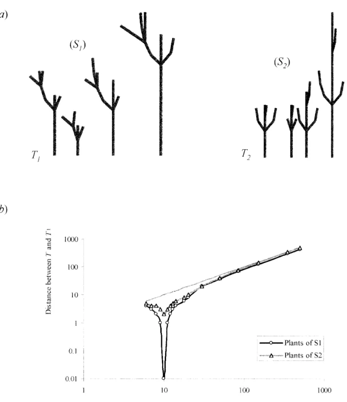
Figure 6. Topological comparison. (a) Sets S₁and S₂of theoretical plants built from T₁and T₂. (b) Distance from plants of S₁and S₂ to reference plant T₁on a logarithmic scale.

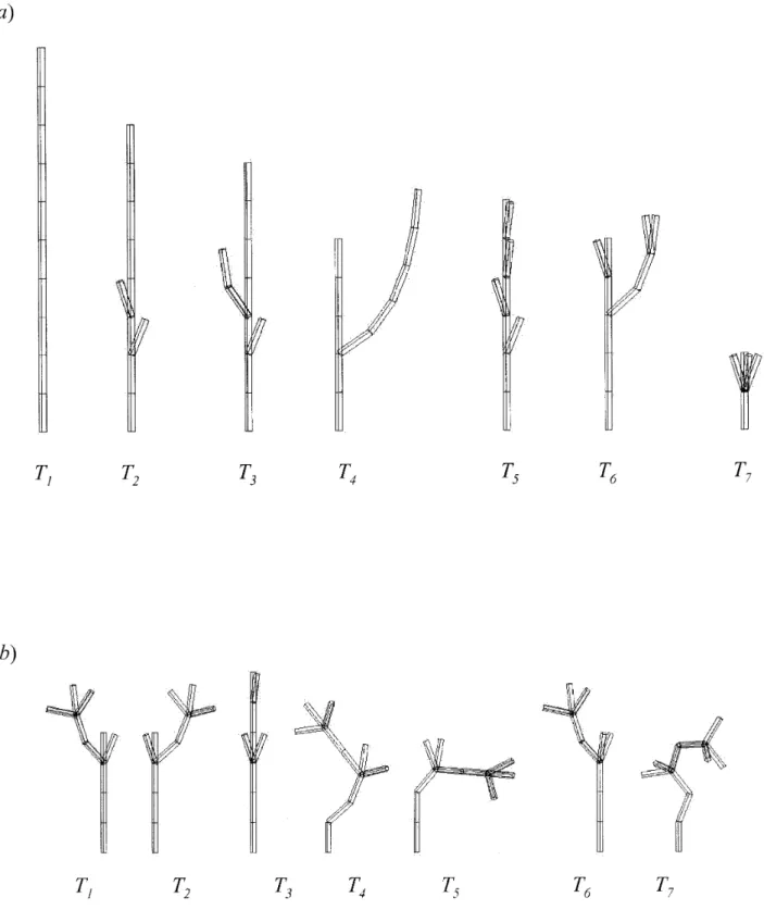
Figure 7. Two sets of theoretical plants: (a) Plants of S₃have different topologies. In the figure, plants are sorted according to their topological similarity to the reference plant T₁. (b) Plants of S₄have a similar topology and different geometry.

organization of the connections between their entities. These differences between two topological structures were evaluated separately using a topological cost which gives results independent of the nature of the entities.

Effect of the number of entities. The effect on the comparison of the difference in the number of plant enti-ties was studied. A reference plant T1made up of ten

ele-mentary entities was constructed. One set of theoretical plants (S1) was generated by decreasing or increasing the

number of entities on each axis of the reference plant. A set of fifteen plants was thus obtained with between six and five hundred entities. A second set (S2) of twelve

plants was defined using the same method for another reference plant T2. Figure 6 shows the distances from the

plants of (S1) and (S2) to the reference plant T1. When the

difference in the number of entities between a given plant and T1is large, the distance between the plants

cor-responds to the difference in their number of elementary entities. Thus, the method proposed in this paper pro-vides interesting information only for plants with a com-parable number of entities.

Effect of connection between entities. If two plants have an equal number of entities, their topological struc-ture may still differ because of the organization of the entity connections. To study this factor, we built two sets of seven theoretical plants containing ten elementary entities in their decomposition. The first set of plants (S3)

contains seven plants and is sorted according to the simi-larity of each plant to the reference plant T1(figure 7a).

The second set gives an example of seven theoretical plants (figure 7b) with a null topological distance between each other but which are geometrically differ-ent. In (S4) each plant is again composed of ten entities.

Plants T1and T2have identical topological structures but different spatial arrangements. Plant T2 is the

mirror-image of T1, i.e. both plants have the same branching

systems but in a symmetric position with respect to a vertical axis. The algorithm gives a null distance between them:

D (T1, T2) = 0. (14)

The spatial ordering of the children of a given entity is not taken into account by the method. Plants T3, T4, T5,

T6and T7have identical topological structures but differ

with respect to the types of connections between their entities. The algorithm based on a topological cost does not distinguish the different types of connections (“+” or “<”) between two entities. However, to make such a dis-tinction with the algorithm, an attribute must be associat-ed with each entity representing the connection relation between the entity and its father. A local cost depending on this attribute would thus take into account the type of connections between entities. These connections often

influence the geometrical disposition of the entities. For example, a series of entities connected by a link “<” is an axis which often can be represented as a straight seg-ment. Such a local cost allows us to account for part of the geometric description of the entities in plants.

5.2 Effect of the local cost function

In the previous section, we compared the topological structures of plants without knowing the nature of the entities. This nature can be taken into account by defin-ing a local distance based on the attributes of the entities. The local cost function may vary by two major parame-ters, the choice of the entity features (e.g. length, diame-ter) and the insert-delete cost. Different changing costs are defined as shown in (11) and (13) to evaluate the influence of attributes. The different values of the insert-delete cost are discussed later.

Effect of attributes. Set (S3) was used to study the

effect of different local cost functions (figure 7a). Each entity of each plant was associated with several attributes such as length, diameter, number of internodes. For each attribute fi (i ≥ 1), a local cost function was defined as follows:

di(v1, v2) = |fi(v1) – fi(v2)| (15)

dins, i(v1) = fi(v1) and ×ddel, i(v2) = fi(v2). (16)

The above algorithm was used to compare plants with the different local cost functions, including a Levenstein’s distance denoted by d0 [22]. For each di (i ≥ 0), a distance matrix Mi, with a size 7×7, was obtained. The individual elements of Mi, Di(Tk, Tl), are computed according to the definition of the distance given by (7). In order to compare distance matrices, each individual element Di(Tk, Tl) is divided by the distance between T1 and T8 (this pair being arbitrarily chosen).

These normalized distances are denoted by Dn i:

(17)

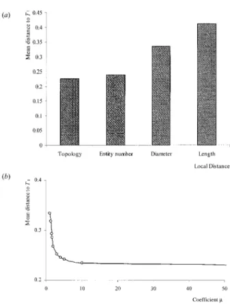
For each fi, the mean distance to the reference plant T1,

denoted by D—n

i, is computed. Figure 8 gives the value of

D—n

i(T1) in different cases. It can be observed that for

attributes showing marked variability, such as the length or diameter entities, the mean distance to T1is very

dif-ferent from the topological mean distance. On the other hand, for attributes such as the number of internodes per growth unit, which are roughly constant over the sets of entities, the computed mean distance is far closer to the topological mean distance.

D_inT_k, T_l = D_f iTk, Tl D_f iT1, T8 .

Effect of insert-delete cost. In equations (11) and (12) several types of insert-delete cost were presented for each local cost function based on a given attribute, that were constant or dependent upon each entity. Set (S3) is

used to study the changes in the distance when the insert-delete cost varies. Hereafter, only the length attribute is considered (the results are similar for other attributes) and the local cost was defined as in (10):

d (v1, v2) = |length (v1) – length (v2)| (18)

(19)

(20)

the evaluation of the mean distance to the reference plants when µ1 is increasing (the same results can be

observed with µ2). When the cost for inserting or

delet-ing increases, the mean distance to a reference plant decreases to a limit value equal to the mean distance to a reference tree when considering topological cost. This limit value is always obtained rapidly and depends on the attribute and the chosen insert-delete cost. If µ1or µ2

are infinite, the normalized distance is equivalent to the normalized distance in the topological case. On the other hand when µ1 or µ2are equal to a minimum value, the

effect of the insert-delete cost on the result reaches a maximum.

6. APPLICATIONS

This section briefly illustrates the use of the compari-son method in different application contexts. The com-parison algorithm discussed in this paper is used as a means to compare the phenotypic expression of plants. To stress the generic character of this method, three examples have been selected for comparing plants with different degrees of genetic distances: the first example illustrates the definition of a distance between groups of plants corresponding to different growth strategies and is based on a comparison of ideal individuals representing the different groups. The second example illustrates the definition of a distance between individuals of a given genus, but with different species. Finally, the third exam-ple sketches out the application of the method in the comparison of hybrid individuals obtained by crossing two fruit tree varieties. Each application outlines different aspects of the comparison algorithm.

From a practical point of view, the user of the com-parison algorithm must first define a local distance between elementary entities. This distance is defined using either real or symbolic attributes of entities. The comparison algorithm can then be used in two different contexts: either to assess the architectural variability of a set of plants or to carry out a piece-by-piece comparison between two plants. When used for sets of plants, the algorithm produces distance matrices that can be ana-lyzed by classical clustering methods, e.g. [15]. For pairs of plants, the algorithm outputs a list of all the matched entities. A detailed analysis of the matched subparts of the plants can then be realized.

dinsv1 =µ2× max v∈T₁∪T₂ length v – min v∈T₁∪T₂ length v ddelv2 =µ2× max v∈T₁∪T₂ length v – min v∈T₁∪T₂ length v . dinsv1 =µ1×length v1 d_delv₂ =µ₁×length v2

Figure 8. Mean distance to the reference plant T₁. (a) Value of the mean distance using several local costs, (b) Changes in the mean distance according to the changes in the insert-delete cost value, the gray line represents the mean distance with a Levenstein’s distance and its asymptote.

Distance between architectural models. In the 1970’s, Hallé et al. [12, 13] proposed to identify a finite number of growing strategies characterizing the develop-ment of tropical plants. Each growing strategy is identi-fied by a growth pattern, called an architectural model, defined by a combination of a limited set of morphologi-cal features [1]: the growth type (rhythmic or continuous growth), the branching pattern (presence or absence of vegetative branching, terminal or lateral branching, monopodial or sympodial branching, rhythmic, continu-ous or diffuse branching), the morphological differentia-tion of axes (orthotropy or plagiotropy) and the posidifferentia-tion of sexuality (terminal or lateral). For example, Corner’s model corresponds to unbranched plants with lateral inflorescences. Up to 23 different models were thus identified corresponding to different combinations of morphological features. Using these concepts, Hallé and Oldeman [12] discussed the relationships between these models reflecting the architectural proximity of certain groups: for example Prévost’s model and Leeuwenberg’s model are claimed to be close since Prévost’s model derives from Leeuwenberg’s model by linear indefinite repetition [12]. Recently, Robinson [31] attempted to formalize the combination of these morphological char-acters by introducing an appropriate coding strategy which underlines the model similarities. For instance, Massart’s model, coded by the chain of symbols (O)r(P), is close to Cook’s model coded by (O)c(P) (where (O) symbolises an orthotropic trunk, r and c respectively rep-resent rhythmic and continuous branching and (P) repre-sents plagiotropic branching). According to Robinson, this formalism defines “an appropriate symbolism that would give a framework within which relationships between the models could be explored”.

In the following application, we show how the pro-posed comparison algorithm can be used as a new method for comparing architectural models. We selected 12 theoretical plants representing 12 different models which can be easily modeled as tree graphs. The plants were defined with the same number of entities. Fruit position and axis orientation were described by corre-sponding attributes associated with each entity. Continuous branching was represented by the presence of one branch on each entity of the trunk, and rhythmic branching was symbolized by two branches on regularly spaced entities of the axes to represent branch whorls. The growth type was not represented here. A local cost was defined depending on axis orientation, fruit position and father-son relationships for each entity with the attributes having identical weights. The 12 plants were compared providing a matrix distance between “mod-els”. The distance between the plants was consistent with the used of a clustering algorithm. The taxonomy tree [2] output by this clustering technique is a tree whose

termi-nal vertices represent the architectural models and the non–terminal vertices represent the distance between the models contained in the sub-trees (figure 9). Three clus-ters can be identified: A Holtum’s cluster containing Corner’s and Chamberlain’s model which is defined by a monopodial or sympodial trunk without branches, a Leeuwenberg’s cluster characterised by a sympodial branching sequence or a true dichotomy, and an interme-diate cluster which contains models such as Massart’s, and Roux’s models (In another interpretation, Scarronne’s model could be isolated in a fourth cluster).

Taxonomy trees between different species or genera usually reflect a genetic distance, e.g. [36]. The compari-son algorithm produces another type of taxonomy tree, reflecting a phenotypic distance between groups of plants.

Clustering of pine families. The piece-by-piece plant comparison algorithm presented here was also used to compare a set of five Pinus nigra and five Pinus halepen-sis, 8-years old, described at growth unit scale, and obtained from simulation (figure 10). Three global vari-ables were associated with each tree, namely the mean length of the tree growth units, the number of tree com-ponents and the number of branches along the trunk. These variables characterize different aspects of the tree morphology. A distance between two trees was defined for each global variables corresponding to the difference between the values for this variable in the two trees. Three matrices were computed for the set of 10 trees, corresponding to these 3 distances. Finally, a fourth matrix distance was computed using the plant compari-son method presented above and Levenstein’s distance.

Then, for each matrix, a classical clustering method [15] was applied to automatically separate the set of 10 pines into two clusters. We compared the obtained clus-ters with the original pine families. We then computed a recognition rate corresponding to the number of individ-uals correctly classified for the 10 individindivid-uals. Figure 11 shows that the recognition rate may vary markedly depending on the considered global variable and that the highest recognition rate (100%) was obtained for the topological comparison. This suggests that plant archi-tectures cannot always be reduced to global variables in applications using plant architecture comparison. A piece-by-piece comparison may in fact be necessary.

Detailed comparison of hybrids. This application is intended to illustrate another aspect of the comparison algorithm output. After a piece-by-piece comparison, the algorithm provides the optimal sequence of edit opera-tions found. The corresponding mapping between the plant entities can be observed using three-dimensional plant reconstruction [9]. Coloring tools used for 3-D rep-resentation provide a feed-back on the detailed matching between elementary tree entities. This type of analysis

showed that some local similarities between two plants can appear in a global comparison. Let us consider for example the mapping resulting from the comparison of two apple tree hybrids measured at internode scale

(figure 12). The parts of the plants shown with identical colors have been mapped onto each other by the compar-ison algorithm and entities in black have been inserted or deleted. This mapping reveals an interesting similarity Figure 9. Taxonomy tree whose

terminal vertices correspond to architectural models and the non–terminal vertices represent the distances between the models appearing on the leaves.

between the two hybrids: the trunk of T1 (in grey) is

more similar to the (grey) branching system of T2than to

the trunk of T2. This suggests that the differentiation

sequence of the meristem which created the T1 trunk is

similar to the differentiation sequence followed by the meristem that created a T2branch. The biologist can use

such results to orient her interpretation of the biological phenomena. In such applications, the comparison method gives the biologist a quantitative overview of the similarity between two plants and a qualitative outline of the similar subparts of both plants.

Figure 10. Three individuals from each pine set: Pinus halepensis on left-hand side and Pinus nigra on right-hand side.

Figure 11. Recognition rate of the clustering algorithm for

dif-ferent definitions of the distance between individual pine trees: (a) distance defined as the difference of growth units, (b) ditto but using the total number of branches on the trunk, (c) ditto but using the number total number of growth unit, (d) distance defined by the piece-by-piece comparison algorithm using a Levenstein’s distance.

Figure 12. Detailed analysis: Each internode of the apple tree

on the left-hand side is colored according to its order: grey for order 1, white for order 2 and 3. Black denotes deleted intern-odes. The matched entities of the second apple tree are colored with the same color as their image and the inserted entities are colored in black. A similarity between the trunk of the first apple tree and a branching of the second plant (in grey color) is outlined by the matching.

into account all information contained in the plant description. In order to express both the modularity and multiscale nature of plant structures and to define a com-parison method according to the topological structure of plants, we used a formalism based on multiscale tree graphs [8]. Another application of this algorithm consists of identifying a branching system in a plant and then proposing an automatic labeling method of a set of plants. The differences between this analytical method and other methods for comparing plants need further investi-gation. The definition of a distance between plants high-lights some general aspects concerning plant comparison are pointed out: clustering problems, automatic labeling of plant structure and, above all, the evaluation of simu-lated plants. These methods will be a useful and essential tool to improve plant simulation techniques.

8. CONCLUSION

In this paper we propose an analytical methodology for comparing plants at a macroscopic scale. Such a method gives a strong meaning to the concept of similar-ity between plants. The piece-by-piece tree comparison presented here was tested on various plant databases (measured apple trees, simulated and real pines).

This work is part of a project to develop quantitative evaluation tools for plant similarity. Such a tool gives a point of view different from that of global methods and uses the topological structure of plants.

Acknowledgements: We would like to thank Y.

Caraglio for providing us with the database of simulated pines, and for fruitful discussions, E. Costes for provid-ing us with the hybrid database and for her help in per-forming the detailed comparison analysis, and S. Henton for reviewing the English in preliminary versions of the manuscript.

REFERENCES

[1] Barthélémy D., Edelin C., Hallé F., Architectural con-cepts for tropical trees, Chapter in a book: Tropical forests: Botanical dynamics, speciation and diversity, Academic Press London, 1989, pp. 89-100.

[2] Barthélemy J.-P., Guénoche A., Les Arbres et Les Représentations Des Proximités, 1988, Collection Méthode + Programmes, Masson, Paris.

Houllier F., A Functional Model of Tree Growth and Tree Architecture, Silva Fenn. 31 (1997) 297-311.

[6] Edmonds J., Karp R.M., Theoretical Improvements in Algorithmic Efficiency for Network Flow Problems, J. Assoc. Comp. Mach. 19 (1972) 248-264.

[7] Ferraro P., Une méthode de comparaison structurelle d’arborescences non ordonnées, technical report, Cirad (1998), Montpellier.

[8] Godin C., Caraglio Y., A multiscale model of plant topological structures, J. Theor. Biol. 191 (1998) 1-46.

[9] Godin C., Costes E., Caraglio Y., Exploring plant topo-logical structure with the AMAPmod Software: an outline, Silva Fenn. 31 (1997) 355-366.

[10] Godin C., Guédon Y., Costes E., Caraglio Y., Measuring and analyzing plants with the AMAPmod software, Chapter in a book: Advances in computational life sciences, Vol. I: Plants to ecosystems, CSIRO, Australia, 1997, pp. 63-94.

[11] Guédon Y., Costes E., A statistical appraoch for ana-lyzing sequences in fruit tree architecture, Fifth international symposium on computer modelling in fruit research and orchard management (1998), Proceeding, Acta Horticulturae, ISHS.

[12] Hallé F., Oldeman R.A.A., Essai sur l’architecture et la dynamique de croissance des arbres tropicaux, 1970, Paris.

[13] Hallé F., Oldeman R.A.A., Tomlinson P.B., Tropical trees and forests. An architectural analysis, 1978, Springer Verlag, New York, Heidelberg, Berlin.

[14] Hanan J.S., Room P., Practical aspects of plant research, 1997, Australia, Chapter in a book, pp. 28-43.

[15] Kaufman L., Rousseuw P.J., Finding groups in data, 1990, Wiley Series in Probability and Mathematical Statistics.

[16] Kececioglu J.D., Myers E.W., Combinatorial algo-rithms for DNA assembly, Algorithmica 13 (1995) 7-51.

[17] Kilpelläinen P., Mannila H., The Tree Inclusion Problem, 1 (1991) 202-214, Proc. Internat. Joint Conf. on the Theory and Practice of Software Development (CAAP’91).

[18] Kruskal J.B., An Overview of Sequence Comparison, Chapter in Book: Addison-Wesley Publishing Company Inc., 1983, pp. 1-44.

[19] Küppers M., Carbon relations and competition between woody species in a Central European hedgerow, Oecologia 66 (1985) 343-352.

[20] Kurth W., Growth grammar interpreter GROGRA 2.4: A software for the 3-dimensional interpretation of stochastic, sensitive growth grammars in the context of plant modelling, technical report, Forschungszentrum Waldoekosysteme der Universitaet Goettingen (1994).

[21] LeDizès S., Cruiziat P., Lacointe A., Sinoquet H., LeRoux X., Balandier P., Jacquet P., A Model for Simulating Structure-Function Relationships in Walnut Tree Growth Processes, Silva Fenn. 31 (1997) 313-328.

[22] Levenstein A., Binary codes capable of correcting dele-tions, insertions and reversals, Sov. Phy. Dokl. 10 (1966) 707-710.

[23] Levinson S.E., Rosenberg A.E., Levinson S.E., Evaluation of a word recognition system using syntax anlysis, Bell Syst. Tech. J. 57 (1978) 1619-1626.

[24] Lu S.-Y., A tree-to-tree distance and its application to cluster analysis, IEEE Trans. Pattern Anal. Mach. Intell. 1 (1979) 219-224.

[25] Mech R., Prusinkiewicz P., Visual models of plants interacting with their environment, SIGGRAPH 96 Conference Proceedings (1996) 397-410.

[26] Miclet L., Méthodes Structurelles Pour la Reconnaissance Des Formes, 1984, 61 Bd. Saint-Germain, 75005 Paris, 184, Book.

[27] Noetzel A.S., Selkow S.M., An Analysis of the General Tree-Editing Problem, Addison-Wesley Publishing Company Inc., 1983, pp. 237-252.

[28] Ohmori A., Tanaka E., A unified view on tree metrics, Syntactic Struct. Patt. Recognition 45 (1988) 85-100.

[29] Preparata F.P., Yeh R.T., Introduction to Discrete Structures for Computer Science and Engineering, 1973.

[30] Prusinkiewicz P., Lindenmayer A., The algorithmic beauty of plants, 1990, New York.

[31] Robinson D.F., A symbolic framework for the descrip-tion of tree architecture models, Botan. J. Linn. Soc. 121 (1996) 243-261.

[32] Selkow S.M., The tree-to-tree editing problem, Inf. Proc. Lett. (1977) 184-186.

[33] Sinoquet H., Rivet P., Godin C., Assessment of the three-dimensional architecture of walnut trees using digitizing, Silva Fenn. 31 (1997) 265-273.

[34] Sobel E., Martinez H., A multiple sequence alignment program, Nucleic Acid Res. 12 (1986) 75-88.

[35] Stanley R.P., Enumerative combinatorics, 1986, Monterey Vol. 1.

[36] Swofford D.L., Olsen G.J., Phylogeny reconstruction, 1990, Sunderland, Massachussets, USA, 411-501, Chapter in a book: Molecular Systematics, Sinauer Associates, Sunderland, Massachussets, USA.

[37] Tai K.-C., The tree-to-tree correction problem, J. Ass. Comp. Mach. (1979) 422-433.

[38] Tanaka E., Tanaka K., The tree-to-tree editing problem, Internat. J. Patt. Recogn. Artif. Intell. 2 (1988) 221-240.

[39] Tanaka E., Toyama T., Kawai S., High speed error cor-rection of phoneme sequences, Patt. Recogn. 19 (1986) 407-412.

[40] Tarjan R.E., Data Structures and Network Algorithms, Chapter in a book, Regional Conference Series in Applied Mathematics, Murray Hill, New Jersey, USA, 1983, pp. 97-111. [41] Tarjan R.E., Data Structures and Network Algorithms, Chapter in a book: Regional Conference Series in Applied Mathematics, Murray Hill, New Jersey, USA, 1983, pp. 85-96.

[42] Wagner R.A., Fisher M.J., The string-to-string correc-tion problem, J. Ass. Comp. Mach. 21 (1974) 168-173.

[43] Zhang K., A new editing-based distance between unordered trees, 4th CPM’93 Padala, Italy, 1993, pp. 254-265.

[44] Zhang K., A constrained edit distance between unordered labeled trees, Algorithmica 15 (1996) 205-222.

[45] Zhang K., Jiang T., Some MAX SNP-hard results con-cerning unordered labeled trees, Inf. Proc. Lett. 49 (1994) 249-254.