HAL Id: hal-02936152
https://hal.archives-ouvertes.fr/hal-02936152
Submitted on 17 Sep 2020
HAL is a multi-disciplinary open access
archive for the deposit and dissemination of
sci-entific research documents, whether they are
pub-lished or not. The documents may come from
teaching and research institutions in France or
abroad, or from public or private research centers.
L’archive ouverte pluridisciplinaire HAL, est
destinée au dépôt et à la diffusion de documents
scientifiques de niveau recherche, publiés ou non,
émanant des établissements d’enseignement et de
recherche français ou étrangers, des laboratoires
publics ou privés.
Atlantic Meridional Overturning Circulation and δ 13 C
Variability During the Last Interglacial
A. Kessler, N. Bouttes, Didier M. Roche, U. Ninnemann, E. Galaasen, J.
Tjiputra
To cite this version:
A. Kessler, N. Bouttes, Didier M. Roche, U. Ninnemann, E. Galaasen, et al.. Atlantic Meridional
Over-turning Circulation and δ 13 C Variability During the Last Interglacial. Paleoceanography and
Paleo-climatology, American Geophysical Union, 2020, 35 (5), pp.e2019PA003818. �10.1029/2019PA003818�.
�hal-02936152�
A. Kessler1 , N. Bouttes2 , D. M. Roche2,3, U. S. Ninnemann4 , E. V. Galaasen4 ,
and J. Tjiputra1
1NORCE Norwegian Research Centre, Bjerknes Centre for Climate Research, Bergen, Norway,2Laboratoire des
Sciences du Climat et de l'Environnement, LSCE/IPSL, CEA-CNRS-UVSQ, Université Paris-Saclay, Gif-sur-Yvette, France,3Department of Earth Sciences, VU University Amsterdam, Amsterdam, The Netherlands,4Department of
Earth Science, University of Bergen and Bjerknes Centre for Climate Research, Bergen, Norway
Abstract
The Atlantic Meridional Overturning Circulation (AMOC) is thought to be relatively vigorous and stable during Interglacial periods on multimillennial (equilibrium) timescales. However, recent proxy (δ13C benthic) reconstructions suggest that higher frequency variability in deep watercirculation may have been common during some interglacial periods, including the Last Interglacial (LIG, 130–115 ka). The origin of these isotope variations and their implications for past AMOC remain poorly understood. Using iLOVECLIM, an Earth system model of intermediate complexity (EMIC) allowing the computation of δ13C
DICand direct comparison to proxy reconstructions, we perform a transient
experiment of the LIG (125–115 ka) forced only by boundary conditions of greenhouse gases and orbital forcings. The model simulates large centennial-scale variations in the interior δ13C
DICof the North
Atlantic similar in timescale and amplitude to changes resolved by high-resolution reconstructions from the LIG. In the model, these variations are caused by changes in the relative influence of North Atlantic Deep Water (NADW) and southern source water (SSW) and are closely linked to large (∼50%) changes in AMOC strength provoked by saline input and associated deep convection areas south of Greenland. We identify regions within the subpolar North Atlantic with different sensitivity and response to changes in preformed δ13C
DICof NADW and to changes in NADW versus SSW influence, which is useful for proxy
record interpretation. This could explain the relatively large δ13C gradient (∼0.4%0) observed at ∼3 km
water depth in the subpolar North Atlantic at the inception of the last glacial.
1. Introduction
Variation in the Atlantic Meridional Overturning Circulation (AMOC) is one of the major driving force controlling climate changes as it affects the distribution of heat and carbon in the ocean, thus influencing regional climate and atmospheric CO2concentrations (Ganachaud & Wunsch, 2000). This has made AMOC changes a key concern in future projections, with models suggesting it will likely decrease in response to buoyancy gain in the deep-water formation regions but the extent to which remains highly uncertain (Bakker et al., 2016; Stocker et al., 2014). Meanwhile, recent observations hint that the ocean circulation may have already started changing (Caesar et al., 2018; Smeed et al., 2014).
Analyzing past variability of AMOC can inform us on its stability and tendency to change. The Interglacial periods of the late Pleistocene are particularly interesting in this regard as they shared overall similar bound-ary conditions with the modern climate (Berger et al., 2015). The climate of the Last Interglacial (LIG), or Marine Isotope Stage (MIS) 5e in isotopic marine series, also shared similar features with the model pro-jections of our future climate if anthropogenic greenhouse gas emissions continue unabated: high-latitudes warming (Hoffman et al., 2017; Otto-Bliesner et al., 2013), reduction of Greenland ice-sheet, and higher sea level (Kopp et al., 2009; Otto-Bliesner et al., 2006). Hence, the high-latitude changes occurring during the warm MIS 5e could provide additional insight on AMOC variability. Data reconstructions from this period (130–115 ka) characterize this circulation with a periodically warmer and fresher than today's North Atlantic water (Hoffman et al., 2017; Otto-Bliesner et al., 2006). Reconstructions of millennial-timescale variability indicate that vigorous North Atlantic Deep Water (NADW) production persisted on millennial timescales (Adkins et al., 1997; Oppo et al., 1997), simulztaneously as southern source waters (SSWs) expanded
Key Points:
• Similar variations of bottom water
δ13C to that depicted by data reconstructions are simulated in the North Atlantic for the LIG period • Changes in AMOC strength may be
a key process in distributingδ13C in the ocean interior
• Magnitude of local bottom water
δ13C response depends on position relative to water mass geometry
Correspondence to:
A. Kessler,
Citation:
Kessler, A., Bouttes, N., Roche, D. M., Ninnemann, U. S., Galaasen, E. V., & Tjiputra, J. (2020). Atlantic meridional overturning circulation andδ13C
variability during the last interglacial. Paleoceanography and
Paleoclimatology, 35, e2019PA003818. https://doi.org/10.1029/2019PA003818
Received 19 NOV 2019 Accepted 15 APR 2020
Accepted article online 23 APR 2020
©2020. The Authors.
This is an open access article under the terms of the Creative Commons Attribution License, which permits use, distribution and reproduction in any medium, provided the original work is properly cited.
Paleoceanography
10.1029/2019PA003818
northward at depth towards 115 ka and the last glacial inception (Govin et al., 2009). The influence of Atlantic surface water into the Nordic Seas and farther north into the Arctic Ocean is also suggested to have occurred during the late MIS 5e (Van Nieuwenhove et al., 2011).
The shorter term transient behavior of the ocean circulation during this warmer period remains, however, poorly constrained as is it difficult to robustly identify and assess such short-timescale variability in the marine record. Nevertheless, new generations of high-resolution (down to multidecadal) proxy reconstruc-tions, more appropriate to resolve multicentennial variability, suggest the existence of centennial short-lived large perturbations of the NADW during previous interglacial periods (Galaasen et al., 2014; Hodell et al., 2009; McManus et al., 1999; Ninnemann & Charles, 2002). Data reconstructions of δ13C—an ocean
circu-lation and carbon cycle tracer—from sediment cores in the North Atlantic depict abrupt centennial-scale variations on the order of 0.7%0, comparable to the deep Atlantic δ13C changes observed during glacial
peri-ods and associated with changes in the distribution and ventilation of NADW (Henry et al., 2016; McManus et al., 1999, 2004; Menviel et al., 2017). This suggests possibly large and abrupt variations in ocean ven-tilation, which challenges the paradigm of the stability of interglacial thermohaline circulation at short timescales (Galaasen et al., 2014; Hodell et al., 2009). While the existence of such AMOC change is consis-tent with some observed climate variability (Bauch et al., 2011; Galaasen et al., 2015; Mokeddem et al., 2014; Tzedakis et al., 2018; Zhuravleva & Bauch, 2018), the relationship between benthic δ13C and ocean
circula-tion is not straightforward and requires addicircula-tional tool such as model simulacircula-tions to evaluate their degree of interactions (Bakker et al., 2015).
With respect to the model-data comparison, numerous studies have analyzed the δ13C distribution variations
under various boundary conditions using, for example, two-dimensional ocean models (Bouttes et al., 2009, 2010, 2012; Brovkin et al., 2007) and more complex three-dimensional models (Bakker et al., 2015; Menviel et al., 2017). These studies propose linkages between the millennial-scale variations of δ13C and changes
in a number of processes such as water mass distribution changes (which can be due to interaction with sea-ice formation), biological activity changes (e.g., due to iron fertilization), and land vegetation modifica-tion. However, to the authors' knowledge, there are no modeling studies, which simulate abrupt and large modification in the bottom water δ13C with the amplitude and timescale depicted by the high-resolution
reconstruction data (Galaasen et al., 2014; Hodell et al., 2009), such as shown here. Such constraints are needed to assess, for example, whether it is mechanistically plausible for changes in water mass distribu-tion to have driven abrupt centennial-scale variability in bottom water δ13C and, furthermore, whether such
tracer field adjustments could be linked to AMOC variability. Determining the characteristic pattern or fin-gerprint in interior ocean δ13C related to AMOC changes would provide a more realistic and physically
consistent framework for interpreting past circulation variability and its implication for the carbon cycling but also in understanding its recent (Caesar et al., 2018) and potential future changes (Weijer et al., 2019). Here, we span this knowledge gap by using iLOVECLIM, an Earth system model of intermediate complexity (EMIC), to perform a transient simulation of the LIG (125–115 ka) under past natural variations in natural greenhouse gases and transient orbital forcings.
The paper is organized as follows: In section 2, we describe the model, the experiment design, and the terms and metrics used to analyze the water mass geometry in the interior ocean during the transient simulation. Section 3 presents the results of the model simulations, while discussions and comparison with previous studies are presented in section 4. Finally, the study is summarized in section 5.
2. Method
2.1. Model Description
This study uses the Earth system model of intermediate complexity iLOVECLIM, a LOVECLIM model branch that also includes carbon isotopes. The atmosphere, ocean, and vegetation components are simi-lar to that in LOVECLIM version 1.2 (Goosse et al., 2010; Roche et al., 2007). The atmospheric component ECBilt was developed at the Dutch Royal Meteorological Institute (Opsteegh et al., 1998) and is composed of three vertical layers at 800, 500, and 200 hPa and has a horizontal resolution of 5.6◦. To better represent the dynamics of the Hadley cell, ageostrophic terms are added to the quasi-geostrophic approximation dynami-cal core. The oceanic component CLIO has a horizontal resolution of approximately 3◦and adopts 20 levels on the vertical coordinate including a realistic bathymetry. The oceanic general circulation model (Goosse & Fichefet, 1999) is based on Navier-Stokes equations and includes a parametrization for down-sloping currents (Campin & Goosse, 1999) and an updated version of the thermodynamical sea-ice component of
Fichefet and Maqueda (1997, 1999). The terrestrial biosphere model (VECODE) is composed of three sub-models that exchange heat, stress, water, and carbon and are designed for long-term simulations (Brovkin et al., 1997). In addition to desert, the dynamic vegetation model simulates two types of plants—trees and grass—which are subdivided into four compartments (leaves, wood, litter, and soil) that exchange carbon in the biogeochemical model. The model of vegetation structure computes the fraction of plant functional type (PFT) in equilibrium with the climate where photosynthesis depends on precipitation, temperature, and atmospheric CO2.
The ocean carbon cycle model is divided into organic and inorganic parts that are based on the nutrient-phytoplankton-zooplankton-detritus (NPZD) model described in Six and Maier-Reimer (1996). The inor-ganic carbon is represented by the dissolved inorinor-ganic carbon (DIC) and alkalinity (ALK), while the orinor-ganic part includes phytoplankton, zooplankton, dissolved organic carbon (DOC), slow dissolved organic carbon (DOCs), particulate organic carbon (POC), and calcium carbonate (CaCO3). The plankton is partially
rem-ineralized as it sinks through the water column, while all the POC and CaCO3are remineralized at depth.
The remineralization profile follows an exponential law; however, it is adjusted to have less remineraliza-tion in the upper layers and more at depth. At the air-sea interface, the carbon flux is computed from the CO2partial pressure (pCO2) difference between the atmosphere and the ocean at a constant gas exchange coefficient of 0.06 mol·m−2·yr−1. The sea surface pCO
2is a function of temperature, salinity, DIC, and ALK
following Millero (1995). The iLOVECLIM model is using a similar carbon cycle as in CLIMBER-2 where the13C is computed in the ocean and terrestrial biosphere as in Brovkin et al. (2007) and is fully described
in Bouttes et al. (2015).
2.2. Experiment Set Up
We have performed a transient experiment over the 125- to 115-ka period of the LIG by prescribing yearly interpolated values of greenhouse gases (CO2, CH4, and N2O) and orbital forcings from the third phase of the Paleoclimate Modelling Intercomparison Project (PMIP3; https://pmip3.lsce.ipsl.fr/). This experiment is branched off after two consecutive runs in order to set the initial conditions: (1) a preindustrial spin up fol-lowed by (2) an equilibrium experiment using 125-ka boundary conditions. Both experiments (1) and (2) are simulated over 5,000 model years. The preindustrial spin-up reproduces well the main ocean carbon cycle characteristics and is similar to that described in Bouttes et al. (2015). The atmospheric δ13C and CO
2
con-centrations are −6.5%0 and 282 ppm, respectively, while the ocean and terrestrial biosphere carbon content are 38,952 and 2,094 PgC. The most important features of the different water masses are reproduced and the oceanic δ13C (δ13C
DIC) is relatively well simulated as compared to the data (Eide et al., 2017; Schmittner et
al., 2013), with higher δ13C at the surface due to photosynthesis and lower δ13C in the deeper ocean where
remineralization takes place (Figure 1a). It also depicts the water mass characteristics of NADW (high δ13C)
and Antarctic Bottom Water (AABW; low δ13C) and the equatorial subsurface minimum induced by strong
remineralization. However, the high δ13C values from the NADW penetrate further south in the data
recon-struction (Figure 1b) than that simulated in our model, which is likely the result of too strong diffusion in the model (Bouttes et al., 2015). In other regions, the magnitude and the large-scale spatial pattern of the δ13C
DICtracer are fairly comparable to the observations.
In the 125-ka equilibrium run, that is, experiment (2), the model simulation reaches equilibrium after 3,000 model years where the ocean and land vegetation carbon content stabilize at 38,857 ± 1 PgC and 23,235 ± 4 PgC, respectively, over the proceeding 2,000 simulation years. The atmospheric CO2and the other
green-house gases are kept constant (CO2= 276 ppmv; CH4= 640 ppb and N2O = 263 ppb). The end of the 125-ka
equilibrium run is used as a starting point for the 125- to 115-ka transient simulation. Changes into the car-bon reservoirs are simulated during this period corresponding into a reduction of the ocean carcar-bon content at 125 ka as compared to 115 ka of about 360 PgC. This value is of the same order of magnitude with that suggested by previous studies analyzing the ocean carbon system during the LIG, for example, Schurgers et al. (2006) and Kessler et al. (2018) with 310 and 314 PgC, respectively. However, contrary to the data recon-struction that shows relative stable atmospheric CO2concentration around 270–280 ppm throughout the LIG (Lourantou et al., 2010; Schneider et al., 2013), our model simulates an increase after 123.5ka until it stabilizes again around 116 ka to 305 ppm (nearly 30 ppm above the data reconstruction). This increase is attributed to the strong reduction in land vegetation carbon content (∼420 PgC) induced by gradual cooling of the Northern Hemisphere (∼2◦C) and potentially the absence of permafrost in the model.
Paleoceanography
10.1029/2019PA003818
Figure 1. Atlantic section of preindustrialδ13C (a) simulated by iLOVECLIM (δ13CDIC) and (b) data reconstruction (Eide et al., 2017).
We note that this experiment has also been used in Galaasen et al. (2020) to illustrate the similarity between simulated and reconstructed bottom water δ13C changes in recent interglacials. Hereafter, we provide a
detailed analysis of this simulation defining the cause of the simulated δ13C
DIC anomalies, their spatial
patterns in the deep North Atlantic, and potential drivers of δ13C
DICvariability. 2.3.𝛅13C Tracer
The δ13C represents the standardized13C/12C ratio (Zeebe & Wolf-Gladrow, 2001) and is expressed in permil
units as follows: δ13C = ( (13C∕12C) (13C∕12C) standard −1 ) × 1, 000, (1) where (13C/12C)
standardis the Pee Dee Belemnite carbon isotope standard (Craig, 1957). Hereafter, we con-sider the δ13C of DIC in the ocean, noted δ13C
DIC. During the photosynthesis, marine and terrestrial biology
preferentially use the lighter12C over13C. When organic matter is remineralized at depth, more12C is
released as compared to13C, thus producing low δ13C
DIC. On the opposite, at the surface ocean, the excess
sequestration of12C, relative to13C, during photosynthesis drives an increase in δ13C
DIC. Thus, the
distri-bution of δ13C
DICis affected by air-sea gas exchange and marine biological fractionation (Eide et al., 2017;
Lynch-Stieglitz et al., 1995; Schmittner et al., 2013; Zhang et al., 1995) and as other oceanic tracers, is transported by the advection-diffusion scheme in the oceanic model. The analysis of δ13C
DICis often used
to reconstruct the variations in ocean circulation (Duplessy et al., 1988) and strength of biological pump (Crucifix, 2005; Curry & Oppo, 2005; Eide et al., 2017; Morée et al., 2018).
2.4. Phosphate Oxygen Tracer (PO)
The phosphate oxygen tracer (PO) as defined by Broecker (1974) is a measure for identifying water masses. It is computed using the simulated phosphate and oxygen fields:
PO = O2+rO∶PPO4, (2)
where rO:P is the oxygen-to-phosphate stoichiometric ratio, which is varying from 138 (surface) to 170
(bottom), in the model. For a given water mass, this tracer is presumed to be approximately constant and is based on the principle that phosphate is released while oxygen is used during remineralization, and vice versa during biological production. The distinction of water masses using PO is useful for contrasting inte-rior water masses with very different surface PO values. Here, we mainly use PO to identify northern source water (NSW) and SSW masses in the deep ocean below 1,000 m depth characterized by low and high PO values, respectively.
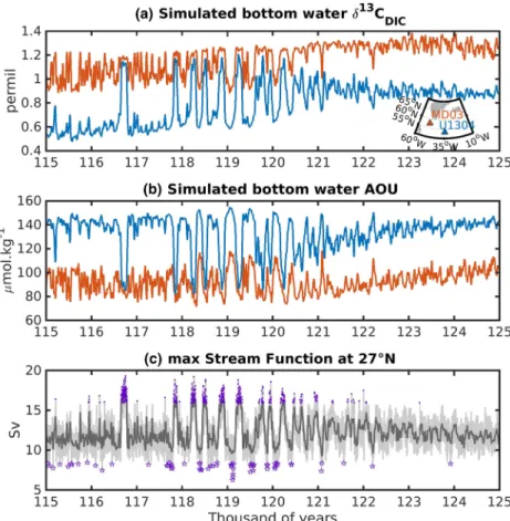
Figure 2. MD03 and U1304 sediment core locations time series of (a) bottom waterδ13CDIC, (b) AOU, and (c) maximum overturning stream function at 27◦N of the North Atlantic. The locations of both sediment cores is shown on the map panel (a). The purple points (stars) represent the years where the maximum stream function is two standard deviations above (below) the long-term mean. A locally weighted linear regression over 40 years is used and shown by the thick lines.
2.5. Apparent Oxygen Utilization (AOU)
The apparent oxygen utilization (AOU) is a diagnostic biogeochemical tracer that provides an estimate of the amount of oxygen used since a water parcel was last at the surface and hypothetically fully saturated. It is computed according to
AOU = Osat2 −O2, (3)
where Osat
2 is the saturation value and O2is the in situ oxygen value calculated by the model. When a water
parcel is advected to the interior, remineralization processes start and consume the oxygen. The older a water parcel, the more oxygen has been consumed by remineralization; hence, AOU increases.
3. Results
Section 3.1 describes the simulated variability in δ13C
DIC and AMOC strength, while a composite
analy-sis opposing strong versus weak AMOC is discussed in section 3.2. The mechanisms associated with the variability of the meridional overturning circulation are addressed in section 3.3. In order to compare and contrast our simulation with data records, we focus our discussion to the locations of the two high-resolution proxy records MD03-2664 (Galaasen et al., 2014) and Integrated Ocean Drilling Program (IODP) Site U1304 (Hodell et al., 2009), which depict centennial-scale δ13C perturbations during the LIG. The location of these
two sites is shown, for instance, in Figure 2a.
3.1. AMOC and𝛅13C Transient Variability
The time series of simulated δ13C
DICat the two sediment core locations are shown in Figure 2a. The absolute
values of δ13C
Paleoceanography
10.1029/2019PA003818
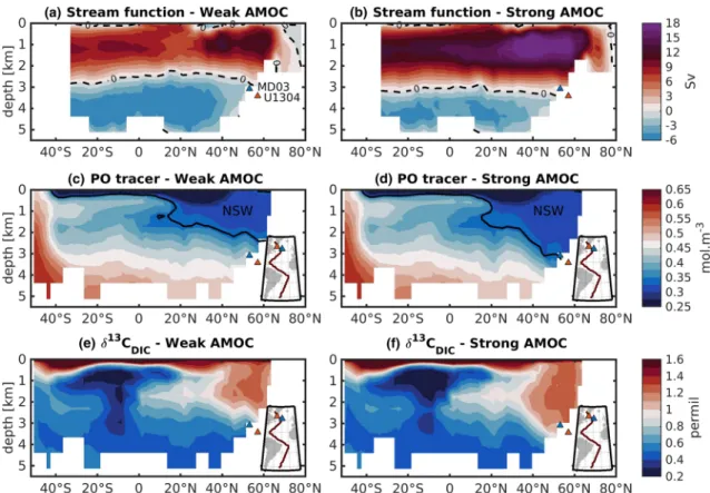
Figure 3. Atlantic section of (a,b) overturning stream function, (c,d) PO tracer, and (d,e)δ13CDIC. The panels on the left (a,c,e) correspond to the average over all the years of weak AMOC (i.e., two standard deviations below the long-term mean). The right side panels (b,d,f) correspond to the strong AMOC points average (i.e., two standard deviations above the long-term mean). The black dashed- lines on the top panels represent the zero line and symbolize the separation between the upper to bottom cells. In the middle panels, the region above the black solid lines show the approximate area that is predominantly occupied by NSW. The value (∼0.36 mol m−3) represents the averaged surface PO over the sinking region south of Greenland.
in maximum values to a relative similar value (e.g., 116.8 and 117.8 ka). In addition, both MD03-2664 and U1304 sites show similar evolution during the transient simulation. While δ13C
DICis relatively stable from
125–122ka (1.28 ± 0.05%0 at MD03-2664 and 0.96 ± 0.04%0 at U1304), stronger variations are simulated during the second half of the experiment where the standard deviation is increased by a factor of three at U1304 and two at MD03-2664. These abrupt changes in bottom δ13C
DICare simulated at centennial timescale
for both locations and show a maximum amplitude of variation of about 0.65%0 and 0.43%0 around 119 ka. This is comparable to the changes depicted by the proxy reconstruction at MD03-2664 (Galaasen et al., 2014), which also highlights similar centennial variations of about 0.7 %0 of magnitude. In addition, small decreasing trend are simulated at MD03-2664 (3.2 × 10⁻⁵%0·yr−1) and U1304 (3.5 × 10⁻⁵%0·yr−1), which
is attributed to the long-term decreasing trend of the atmospheric δ13C and the decreasing land vegetation
carbon reservoir.
The variations in bottom water δ13C
DIC at both locations follow the same variations as depicted by AOU
(Figure 2b). Site U1304 simulates in general higher AOU (∼ 40%) than that at MD03-2664, suggesting that the water mass affecting Site U1304 is more remineralized than at MD03-2664. However, during the abrupt transitions, the difference between both sites is reduced, meaning that both sites are affected by a water mass that has been similarly ventilated (i.e., similar water mass).
Figure 2c shows the evolution of maximum overturning stream function at 27◦N in the Atlantic basin with an averaged value of 12.2 ± 1.8 (one standard deviation) Sv and shows similar variations to those depicted with δ13C
DICand AOU. High values of overturning stream function coincide with high bottom water values
of δ13C
DICat both sediment core sites, which seem to converge toward the same δ13CDICvalue. Conversely, a
weak overturning stream function corresponds to lower values of δ13C
DICand lead to a divergence of δ13CDIC
values between the two core locations. This suggests that the temporal variation of δ13C
DIC in the North
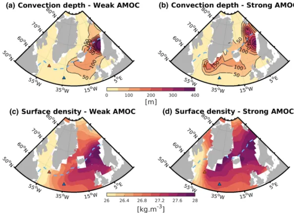
Figure 4. Convection (top panels) and neutral density (bottom panels) at the surface averaged over weak (a,c) and strong (b,d) AMOC years. The light blue dashed lines represent the 15 cm sea-ice thickness limit, as a proxy for sea-ice cover.
In order to further analyze the impact differences in AMOC strength have on the biogeochemistry and ocean δ13C
DIC, we show a composite analysis of two contrasting states of AMOC, that is, weak versus strong AMOC.
For this, we average all years where AMOC strength is two standard deviations above or below the long-term mean. The selected years with strong AMOC states are represented by the purple points (Figure 2c; number of point n = 460), while the selected years with weak AMOC states are shown by the purple stars (n = 63).
3.2. Composite Analysis: Weak Versus Strong AMOC
Figure 3 depicts the vertical structure of the AMOC, PO, and δ13C
DICdistribution along the Atlantic section.
The left panels (Figures 3a, 3c, and 3e) correspond to the average values over weak AMOC years, whereas the right panels (Figures 3b, 3d, and 3f) correspond to the average over strong AMOC years. Under weak AMOC, the separation between the top and bottom cells of the overturning stream function reaches approximately 3,000 m depth around the sediment core locations (Figure 3a, black dashed line). The maximum of the upper cell reaches 13.8 Sv, while the minimum of the bottom cell is about −8.1 Sv. During strong AMOC state, the upper cell is increased as high as 20.5 Sv and deepens by about 400 m depth down to 3,400 m (Figure 3b, black dashed line), while the bottom cell contracts and becomes less vigorous. The blue (red) shade of the PO tracer illustrates the signature of NSW (SSW). NSW affects the region of the sediment cores more strongly when the AMOC is strong (Figures 3c and 3d). This result is in good agreement with the deepening of the upper cell of the AMOC previously mentioned. We note that in both cases, the NADW (NSW) is sustained depicting its relative PO signature down to 2,300 (3,000) m depth under weak (strong) AMOC state. In addition, because NSW has higher δ13C
DIC values than SSW, δ13CDIC-rich water masses
dominate MD03-2664 and U1304 locations when the AMOC is strong (Figure 3f), which is consistent with the convergence of δ13C
DICvalues at both core sites previously mentioned (section 3.1). On the other hand,
more low δ13C
DICwater masses, resulting from the mixing of SSW and NSW, are affecting the sediment cores
during periods of weaker AMOC (Figure 3e).
These two AMOC states are characterized by distinct differences in the location, area, and depth of con-vection in the North Atlantic. In the case of weak AMOC, deep concon-vection is simulated in the Norwegian sea (>400 m depth; Figure 4a), while an area of shallower convection extends further south into the North
Paleoceanography
10.1029/2019PA003818
Figure 5. Sea surface temperature (SST; top panels) and salinity (SSS; bottom panels) averaged over the weak (a,c) and strong (b,d) AMOC years. The light blue dashed lines represent the 15 cm sea-ice thickness limit.
Atlantic. Conversely, under strong AMOC periods, the Irminger Sea region including the southeast Labrador Sea also experiences deep convection down to 150 m depth (Figure 4b), while the convection depth in the Norwegian Sea slightly weakens to 300 m and extends further north under the sea-ice limit. The strongest sea-ice retreat (up to 10◦northward) is simulated in the Irminger Sea and coincides with the activation of convection in this region (Figure 4, light blue dashed lines). The changes depicted by the density field (Figures 4c and 4d) correspond to the changes in convection depth. Under simulated weak AMOC, the densest water masses are in the Norwegian Sea with values of neutral density up to 27.8 kg·m−3where
the convection occurs. When the AMOC strengthens, the surface density increases south of Greenland and in the Irminger Sea, leading to similar density values with that in the Norwegian Sea (27.8 kg·m−3;
Figure 4d). Thus, the total area of dense water formation in these regions increases during the AMOC strong composite state.
Figure 5 shows the annual mean surface temperature and salinity fields during both strong and weak AMOC states. It reveals that lower SSTs are simulated in the regions corresponding to the subpolar gyre (Irminger Sea and southeast of the Labrador Sea) and in the Norwegian Sea when the AMOC weakens (Figures 5a and 5b). For example, the 0◦C isotherm shifts north by about 10◦between Greenland and Norway while it only moves north by about 2◦in southeastern Labrador Sea (Figure 5b). On the other hand, the warmest waters expand westward (i.e., isotherm 8◦C) when AMOC strengthens and onset/increase of convection in the Labrador Sea/Irminger Sea. This suggests strong negative buoyancy flux in these regions due to the heat loss. The SSS field also depicts strong modification in the North Atlantic, especially in the region where the convection turns off and on (Figures 5c and 5d). Under weak AMOC, the strongest SSS (>35.5 psu) are simulated around the Celtic Sea and extend northward toward the Norwegian Sea (Figure 5c), while fresher polar surface waters (<33.6 psu) are being transported along the eastern Greenland coastline following the sea-ice extent. When the AMOC strengthens, the high surface salinity spreads further north into the Norwe-gian Sea and west toward the Irminger Sea and the entrance of the Labrador Sea (Figure 5d). This suggests that more warm and salty surface Atlantic water is entering the Norwegian Sea under stronger ocean circu-lation and recirculates to the northwestern basin following the northward shift of the sea-ice edge between
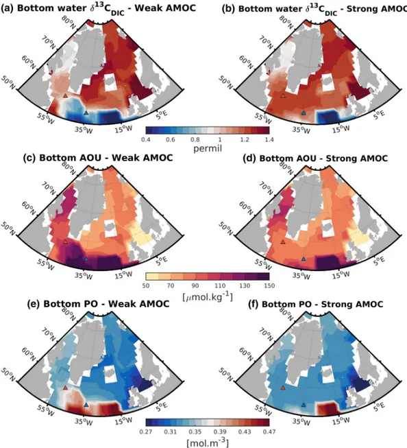
Figure 6.δ13CDIC(top panels), AOU (middle panels), and PO (bottom panels) averaged fields at the sea floor during the weak (left hand side) and strong (right hand side) AMOC years.
Greenland and Iceland (Figure 5d). These increases in SSS cause the surface density to increase, reducing the stratification of the ocean and establishing favorable conditions for deep convection to occur.
While changes in AMOC are expressed clearly in δ13C
DICat both locations (Figures 2a and 2c), the model
predicts slightly different responses at these locations due to the position of the sites relative to major water mass pathways. MD03-2664 is located further North and West and is more influenced by NSW during both strong and weak AMOC composite states (Figures 6e and 6f). Thus, during weak composite states, bottom water δ13C
DICat MD03-2664 does not drop as low as at U1304, which has much greater influence of SSW
than MD03-2664. Figure 6 reveals these differences by depicting the changes in δ13C
DIC, AOU, and PO
trac-ers at the sea floor. The pattern of these three tractrac-ers are strongly similar showing that δ13C
DICchanges are
related to water mass geometry. Under weak AMOC states, MD03-2664 depicts 105.0 μmol·kg−1of AOU
when U1304 has 146.1 μmol·kg−1(Figure 6c), corresponding to 28% of difference. This difference is reduced
to 13% when the AMOC strengthens (Figure 6d); that is, the AOU values in MD03-2664 and U1304 depict 82.5 and 94.6 μmol·kg−1, respectively. However, U1304 AOU values are generally higher than at MD03-2664,
Paleoceanography
10.1029/2019PA003818
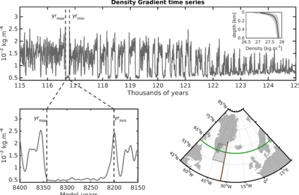
Figure 7. Time series of the vertical density gradient averaged over the first 600 m depth at the location where the convection activates and deactivates south of Greenland (top panel). The subpanel shows the averaged density profile for this area in dark gray thick line, while the standard deviation is depicted by the shaded area. The bottom left panel represents a zoom in on the positive peak of AMOC around 116.7 ka, which corresponds to a negative peak of vertical density gradient. We note yrmin(116.799 ka) the initial year of the upward (downward) trend of the AMOC (vertical density gradient) and yrmax(116.657 ka) the last maximum (minimum) value of the AMOC (vertical density gradient). The area where the convection activates and deactivates is represented in the bottom right panel by the hatched area. The longitudinal and latitudinal sections shown in Figures 8 and 9 are represented by the green and brown solid lines.
during both strong/weak AMOC states. Consequently, the bottom water δ13C
DICvalues simulated at U1304
are lower compared to MD03-2664, and this difference is even more pronounced when the AMOC weak-ens (Figure 2a). Finally, the PO tracer confirms that both sites are affected by different water masses under weak AMOC, while this difference strongly decreases when the ocean circulation strengthens. Thus, under weak AMOC, the MD03-2664 location depicts weaker PO value than at U1304 (Figure 6e; 0.35 against 0.42 mol·m−3, respectively), while almost the same values are depicted under strong AMOC (Figure 6f; 0.32
against 0.34 mol·m−3, respectively). 3.3. AMOC Oscillations
Figure 7 shows the time series of the vertical density gradient for the region where the deep convection turns on and off. The oscillations of the density gradient south of Greenland covary with the AMOC strength during the centennial peak events. As the stratification decreases (density gradient weakens), the AMOC strength increases. In the model, this suggests that the stratification of the ocean south of Greenland is at least partially linked to the AMOC strength during these centennial peaks. The salinity field is the main driver for the changes in density at the surface. The amplitude of oscillations is weaker at the beginning of the simulation than toward 115 ka. The lower values remain relatively constant around 0.5 × 10⁻³kg·m−4
but the maximum values increase toward 115ka (up to 3.6 × 10⁻³kg·m−4), especially after 122 ka. This
increasing trend in maximum of density gradient is attributed to fresher surface ocean simulated toward 115 ka in that area potentially induced by stronger variability in the growing-melting of sea-ice. Hence, the surface salinity in this region is in averaged 2 psu lower in the late LIG (116–115 ka) than at the beginning (125–124 ka). The variation of surface density are more than six times greater at the surface (27.86 ± 0.33 kg·m−3) than at 600 m depth (27.12 ± 0.05 kg·m−3) and are most likely also due to the sea-ice growth and
retreat in this area.
In order to identify the mechanisms behind the changes in surface density, we analyze the onset and off-set of the AMOC peak events. We focus on the event occurring around 116.7 ka as an example because it corresponds to the strongest variation of both AMOC and δ13C
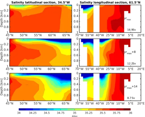
Figure 8. Vertical sections of the salinity in the North Atlantic along (left panels) the longitude 34.5◦W and (right panels) the latitude 61.5◦N. The first row corresponds to the initial year of the upward trend of the AMOC in 116.799 ka (yrmin). The middle row represents the state of the ocean salinity 11 years after the AMOC starts to increase, while the last row corresponds to the end of the onset of this event when the AMOC reaches the nearly maximum (simulated 18 years after yrmin).
Figure 2c shows similar characteristics. We note yrminas the year when the AMOC reaches its last minimum value before increasing (yrmin= 116.799). Similarly, we note yrmaxas the year when the AMOC reaches its last maximum value before decreasing and ending the strong AMOC peak event (yrmax= 116.657, 142 years after yrmin).
Figure 8 depicts the salinity in latitudinal (left panels) and longitudinal (right panels) sections of the North Atlantic Ocean. The first row represents the salinity of the first 1,000 m depth in the North Atlantic Ocean at yrmin. The second row represents the same sections at yrmin+ 11 years of simulation and the last row corresponds to the end of the onset peak at yrmin+ 18 years. These years represent well the changes in the water mass distribution associated to the multidecadal initiation (and offset) of the abrupt transition. Showing any other years within this interval would provide similar results. At the onset of the AMOC peak (yrmin), the AMOC is at the minimum of 9.2 Sv. A 100- to 200-m layer of fresh water extends from the high latitudes down to almost 45◦N and spreads from the Greenland coast eastward to 25◦W leading to a stratified ocean surface (Figure 8, first row panels). This fresh water is associated to sea-ice cover. The Atlantic water corresponds to the higher salinity at 45◦N below 200 m depth (Figure 8). It extents northward along the Norwegian coast and depicts salinity>35.75 psu. At yrmin+ 11 (panels on the second row), the volume of fresh water east of the Greenland coast reduces and starts retreating northward. Similarly, the salinity increases from the eastern side and traces of convection begin to appear around 25◦W, mixing the salinity through the water column. Hence, the AMOC slightly speeds up and increases by +1.7 Sv to reach 10.9 Sv. At the end of the onset (yrmin+ 18), the AMOC is near its maximum (16.7 Sv) and the salinity north of 60◦N increases. By contrast, between 50 and 55◦N, the surface water is simulated fresher and may be associated to the transport of the fresh water from the sea-ice melt. The intrusion of salty water mass seems to originate from the eastern side of the basin where the saline Atlantic waters expand from the Norwegian coast toward the Greenland coastline. As a result, saline Atlantic waters fill up the basin along the 61.5◦N latitude band creating favorable conditions for convection south of Greenland. The same ocean structure is simulated during the time of the maximum AMOC, which corresponds to a 124 years window. Figure 9 is similar to
Paleoceanography
10.1029/2019PA003818
Figure 9. Similar to Figure 8, but for the offset of the upward AMOC trend. Here, yrmaxrepresents the last maximum
value of the AMOC in 116.657 ka (142 years after yrmin) before it starts to decrease to finally reach its minimum at yrmax+ 14.
Figure 8, but represents the offset of the AMOC peak, from yrmaxto the next minimum (yrmax+ 14). This decreasing AMOC phase (increasing stability) mirrors the phase of increasing AMOC (decreasing stability) and shows a gradual establishment of the freshwater layer associated with sea-ice growth. No significant differences compared to the onset could be identified.
4. Discussion
The ocean circulation is one of the key processes affecting the ocean carbon storage, hence regulating the atmospheric CO2levels on millennial timescale. The production of NADW during the LIG is vigorous and
appears relatively robust at (multi)millennial timescales, that is, suggested by numerous of studies. However, new high-resolution proxy records reveal that abrupt changes in bottom water chemistry (δ13C) occurred
on centennial timescales during the previous interglacial and are postulated to represent ocean circulation changes. Yet, it is less clear how these circulation changes relate to AMOC or, indeed, even if deep circula-tion changes could explain such rapid changes in deep Atlantic δ13C—onset and terminated in decade(s)
and generally persisting for one or few centuries (Galaasen et al., 2014). In this study, we simulate a tran-sient experiment from the last interglacial period (125–115 ka) using an Earth system model of intermediate complexity (EMIC) allowing the computation of δ13C
DIC, an oceanic tracer for the ocean circulation, and
biogeochemical processes used in paleoclimate reconstruction. Significant changes of δ13C
DICare simulated
in the North Atlantic at short timescale (centennial), which approach in magnitude those depicted in the data reconstruction. Likewise, the transitions (increases and decreases) also occur quickly, consistent with the rapid onset and demise observed in the proxy reconstruction. The variability in bottom water δ13C
DIC
is found to be positively correlated to the AMOC strength, which oscillates between 6.3 and 19.3 Sv. These AMOC oscillations are mainly controlled by the convection south of Greenland (Labrador Sea and Irminger Sea), which turns off and on with the northward and westward expansion of highly saline Atlantic waters from the Norwegian coast to Greenland around 60◦N, associated with the northward retreat of sea-ice and fresh surface waters.
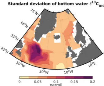
Figure 10. Standard deviation of bottom waterδ13CDICover the entire simulation.
The representation of the North Atlantic ventilation is coherent with that suggested by previous studies. The mid-depth North Atlantic water remains relatively well ventilated during the entire period of simulation, even during the simulated weak AMOC events (Figure 3c). This persis-tent production of NSW at mid-depth from 125 to 115 ka is also suggested by other studies based on proxy reconstructions (McManus et al., 2002; Mokeddem et al., 2014) and previous independent model simulations (Born et al., 2011; Wang & Mysak, 2002). Moreover, our results also sup-port previous interpretations of proxy data concerning the deep North Atlantic water (Galaasen et al., 2014; Hodell et al., 2009), that is, that ven-tilation of the deep Atlantic was intermittently disturbed during the LIG and that AMOC strength and NSW-SSW shifts could plausibly explain North Atlantic deep water δ13C changes during interglacials. Thereby,
as shown in Galaasen et al. (2020), the simulated deep Atlantic δ13C DIC
anomalies are strongly similar in magnitude (0.5–0.7%0) and temporal characteristics (decadal scale at onset and persisting for centuries) to the variability in high-resolution δ13C reconstructions. Assuming that the
reconstructed proxies reasonably capture the core top δ13C values, our
model simulation suggests that the region south of Greenland would be most suitable to capture any apparent variations in the watermass prop-erties over the LIG period while regions located further North and East (e.g., in the Nordic Seas) remains more stable. Figure 10 highlights this point by showing higher bottom water δ13C
DIC standard deviation
south of Greenland as compared to any other regions of the North Atlantic. In our simulation, when AMOC is strong, both sediment core sites are affected by the same water mass (NSW) with similar biophysical prop-erties leading to similar δ13C
DIC values. Conversely, when AMOC weakens, the influence of SSW at Site
U1304 increases; hence, the δ13C
DICvalues of both locations diverge. This suggests that relatively large
dif-ferences in tracer (δ13C) signals between two cores located in relatively close proximity can occur due to
the changes in water mass distributions (NSW vs SSW). Using the same model for the period 132–120 ka, Bakker et al. (2015) have also shown a close correlation between North Atlantic bottom water δ13C
DICand
AMOC strength on multimillennial timescale. Our study further supports this result on (multi)centennial timescale.
In addition to those rapid shifts, the proxy data records from MD03-2664 and Site U1304 show markedly different long-term trends in bottom water δ13C from 122 to 115 ka (see figure 3 in Galaasen et al., 2014).
While bottom water δ13C at MD03-2664 increases through the late LIG, it decreases at Site U1304, resulting
in a gradient of ∼0.4%0 between the western (MD03-2664) and eastern subpolar basins (Site U1304) near 115 ka and the last glacial inception. In our model simulation, the long-term transient trends deviate some-what from the actual sites and show at both location a small decreasing trend. This discrepancy with data reconstruction can be attributed, at least in part, to the coarse spatial resolution of the model and the dif-ficulty to properly simulate overflows in this region. However, much of our model simulation shows deep North Atlantic δ13C
DICgradient of ∼0.4%0 between MD03-2664 and Site U1304 (Figure 2a) similar to the
proxy records toward 115 ka. In the model, this difference is caused by relatively higher influence of SSW in the eastern basin and Site U1304 (Figure 6e), which is restricted by the bathymetry from entering the west-ern basin. Therefore, we suggest that the observed ∼0.4%0 δ13C gradient for the late LIG could be explained
from such water mass geometry state, that is, the expansion of the SSW into the subpolar North Atlantic in the late LIG (Govin et al., 2009).
While similar in character, the forcing of the centennial-scale LIG variability likely differs between the sim-ulated and reconstructed events. The reconstructed variability focuses around the early phase of the LIG and appears closely associated with discharge of freshwater and icebergs, including a freshwater outburst flood event associated with the final retreat of the Laurentide ice sheet (Galaasen et al., 2014; Hodell et al., 2009; Nicholl et al., 2012). In the model, the variability occurs in the mid-LIG to late LIG and is asso-ciated with changes in the distribution of sea ice and freshwater within the subpolar North Atlantic and Nordic Seas. This discrepancy from the proxy data arises mainly from the initial conditions used to begin the transient simulation—equilibrium state at 125 ka—which removes potential effects from reminiscent glacial conditions especially at the beginning of the simulation. Hence, the simulated absolute values of
Paleoceanography
10.1029/2019PA003818
δ13C
DICmay not correspond to the reality from that period. However, the climate response to orbital and
greenhouse gases forcings remain sufficient to create large modifications in the interior ocean carbon distri-bution and water mass geometry, which comes to support the short-lived large perturbations of the climate system under warmer climate conditions than today. These rapid shifts in deep water occur as the inter-nal ocean adjusts to switches in AMOC strength. These shifts in AMOC strength are due to changes in surface ocean convection sites and in particular involve turning on and off convection in the Nordic Seas. Similar variations in overturning geometry and strength tied to the location and strength of deep convec-tion have been invoked previously in particular to explain abrupt, millennial-scale ocean-climate changes observed during the last glacial cycle (Rahmstorf, 2002). Our simulation provides an example of how similar shifts in convection-AMOC strength could explain centennial scale variability seen in proxy records during interglacial boundary conditions.
The multicentennial scale variability of AMOC simulated by our model is closely linked to the occurrence of deep convection events south of Greenland. Here, transport of anomalously saline subsurface water mass leads to a strong AMOC strength while fresher water leads to weaker AMOC. The importance of salinity as well as the magnitude and timescale of the AMOC changes shown here are consistent with previous studies applying ECBilt-CLIO coupled model (Jongma et al., 2007) and LOVECLIM (Friedrich et al., 2010), albeit they use slightly different boundary conditions. Furthermore, our simulation shares some important fea-tures with Friedrich et al. (2010) regarding the behavior of AMOC oscillations and the mechanisms involved in it. Among them is the AMOC preferentially operating at weak state toward 115 ka when the obliquity reduces to 22.4 and its related increase of large abrupt AMOC change occurrences during the second half of the LIG, but also changes of the Greenland-Iceland-Norwegian (GIN) sea overturning circulations (not shown here) ahead of the total AMOC changes. However, our simulation do not show any deep decou-pling from subsurface temperature increase responsible for the AMOC increase, as shown in Friedrich et al. (2010), but rather atmospheric temperature anomalies above the sea level (up to 10 K, not shown here) inducing wind stress anomalies favorable to transporting anomalously saline water south of Greenland as mentioned in Schulz et al. (2007). Here, the origin of density changes and the subsequent activation of deep convection comes rather from a surface salinity change. Hence, the salinity remains to be one of the key factor in triggering the deep convection areas that switches the AMOC from weak to stronger states; the mechanisms behind their origin remain however partially unclear. Further sensitivity experiments are needed in order to fully diagnose the mechanisms responsible for the fresh versus saline water shifts south of Greenland.
5. Conclusion
Recent high-resolution proxy records reveal that abrupt changes in bottom water chemistry (δ13C) occurred
on centennial timescales during the previous interglacial and are postulated to represent ocean circulation changes, thus challenging the paradigm of interglacial thermohaline circulation stability at short timescale (Galaasen et al., 2014; Hodell et al., 2009). In this study, we use the iLOVECLIM Earth system model of intermediate complexity to simulate a transient experiment of the LIG period from 125 to 115 ka to analyze possible mechanisms behind these short-lived disturbances depicted by the δ13C data reconstruction from
that period.
Our simulation depicts large perturbations of bottom water δ13C
DICup to 0.43%0 and 0.65%0 in the North
Atlantic at the locations corresponding to the sediment core sites MD03-2664 (Eirik Drift) and U1304 Site (Gardar Drift), respectively. These variations are strongly similar in magnitude (0.5–0.7%0) and temporal characteristics (multidecadal scale at onset and persisting for centuries) to the variability in high-resolution δ13C reconstruction. The simulated δ13C
DICat both sites generally differ by about 0.4%0, similar to the δ13C
gradient observed in the subpolar North Atlantic during the late LIG. In the model, this gradient is attributed to the relative influence of northern source water (NADW) versus SSW to the sediment core locations. However, during the centennial scales perturbations, the simulated bottom water δ13C
DICvalues converge
toward the same values, suggesting that similar water mass properties could potentially be affecting both sites, which is confirmed by our PO analysis.
The simulated variations in δ13C
DICat MD03-2664 and U1304 Site are correlated to the variations in AMOC
strength, which ranges from 6.3 to 19.3 Sv. High values of bottom δ13C
DIC correspond to strong AMOC
and vice versa. Consequently, a simulated strong AMOC state leads to similar bottom water δ13C
at both locations (i.e., affected by the same water mass—NADW), while when the AMOC decreases, the influence of SSW at U1304 Site increases. These large AMOC differences are linked to the activation and deactivation of convection areas south of Greenland, highlighting the importance of NADW production in this region and its role in redistributing δ13C
DICin the interior ocean.
In our model simulation, the mechanism associated to the activation and deactivation of the convection south of Greenland and therefore the AMOC strength is related to a weakening of the vertical density gra-dient mainly induced by the surface salinity in this region, which increases and decreases along with the sea-ice and associated freshwater extension. Northward intrusions of warm and saline Atlantic water into the Nordic Seas also gradually expand westward from 25◦W toward the Greenland coast. In turn, the sea-ice and associated freshwater surface layer retreats (up to ∼10◦ northward) and the advected saline surface water increases the surface density. This sets favorable conditions for deep convection to occur, initiating the AMOC increase.
While the deep Atlantic δ13C
DIC changes seen in our model simulation and the proxy data are similar in
magnitude and temporal characteristics, several discrepancies and differences can be mentioned. The use as initial conditions of the equilibrium at 125 ka state sets different climate background than it may have been in reality. Consequently, (1) the absolute values of bottom water δ13C
DICare generally simulated higher than
that depicted by the data reconstructions, and (2) the simulation does not reproduce the abrupt variations during the early LIG, potentially due to the lack effects from the final retreat of glacial ice sheet remnants (Nicholl et al., 2012). In addition, our model simulates similar decreasing long-term trends at both sediment core locations that do not correspond to what is observed in the data records depicting different trends at both locations. This is attributed to the simulated strong decline of the land vegetation carbon content (∼420 PgC) towards 115 ka and the associated decrease in atmospheric δ13C. Hence, terrestrial vegetation
content seems to play an important role in setting the ocean δ13C
DICabsolute values, which has also been
highlighted for glacial periods (Menviel et al., 2017). Finally, the abrupt transitions occur when the model switches from a strong AMOC state (early LIG) to a weak state (late LIG) and are likely associated to the cooling (i.e., sea-ice/freshwater forcings) towards the glacial inception at 115 ka, which differs from future projected climate. Additional experiments need to be performed in order to properly address the internal mechanisms shaping the frequency and occurrence of these abrupt transitions. In the model, the typical changes in atmospheric CO2associated with these abrupt transitions are approximately of 7 ppm, which
is in the range of the CO2variation observed in the data reconstruction from that period (Lourantou et al., 2010; Schneider et al., 2013), while the changes in ocean DIC are of about 15 PgC and compensated by a 30 PgC increase in the land vegetation carbon.
This study underlines that during the LIG the Labrador Sea and Irminger Sea may have been sensitive to density changes altering the strength of the AMOC over several decades by simple natural greenhouse gases and orbital forcings, hence affecting the distribution of bottom water δ13C
DIC. These unforced oscillations
may be specific to our simulation and do not exclude other potential mechanism that may be responsible for abrupt and large changes of bottom water δ13C depicted in some marine records. The stronger
ampli-tude of change in δ13C
DIC at U1304 Site as compared to MD03-2664 potentially reveals this location at a
better indicator for AMOC structure and/or strength change. In addition, we highlight the need for more isotope-enabled model simulations over interglacial periods in order to better constrain and link changes observed in the marine records and potential changes in overturning circulation.
References
Adkins, J. F., Boyle, E. A., Keigwin, L., & Cortijo, E. (1997). Variability of the North Atlantic thermohaline circulation during the last interglacial period. Nature, 390(6656), 154. https://doi.org/10.1038/36540
Bakker, P., Govin, A., Thornalley, D. J., Roche, D. M., & Renssen, H. (2015). The evolution of deep-ocean flow speeds andδ13C under large changes in the atlantic overturning circulation: Toward a more direct model-data comparison. Paleoceanography, 30(2), 95–117. Bakker, P., Schmittner, A., Lenaerts, J., Abe-Ouchi, A., Bi, D., van den Broeke, M., et al. (2016). Fate of the Atlantic meridional overturning
circulation: Strong decline under continued warming and Greenland melting. Geophysical Research Letters, 43, 12–252. https://doi.org/ 10.1002/2016GL070457
Bauch, H. A., Kandiano, E. S., Helmke, J., Andersen, N., Rosell-Mele, A., & Erlenkeuser, H. (2011). Climatic bisection of the last interglacial warm period in the polar North Atlantic. Quaternary Science Reviews, 30(15-16), 1813–1818. https://doi.org/10.1016/j.quascirev.2011. 05.012
Berger, A., Crucifix, M., Hodell, D., Mangili, C., McManus, J. F., Otto-Blisner, B., et al. (2015). Interglacials of the last 800,000 years. Reviews
of Geophysics, 54, 162–219. https://doi.org/10.1002/2015RG000482
Acknowledgments
We thank the two anonymous referees for their positive and constructive comments, which helped to clarify the manuscript. We also thank the Editor Stephen Barker for the time he dedicated in processing our manuscript and his additional feedback. This work was supported by the Research Council of Norway funded project THRESHOLDS (254964) and ORGANIC (239965) and Bjerknes Centre for Climate Research project BIGCHANGE. We acknowledge the Norwegian Metacenter for Computational Science and Storage Infrastructure
(Notur/Norstore) projects nn1002k and ns1002k for providing the computing and storing resources essential for this study. The authors declare no conflict of interest.The model data are available on the Norwegian Research Data Archive server (https://doi.org/ 10.11582/2019.00037 Kessler, 2019).
Paleoceanography
10.1029/2019PA003818
Born, A., Nisancioglu, K. H., & Risebrobakken, B. (2011). Late Eemian warming in the Nordic Seas as seen in proxy data and climate models. Paleoceanography, 26, PA2207. https://doi.org/10.1073/pnas.1322103111
Bouttes, N., Paillard, D., & Roche, D. (2010). Impact of brine-induced stratification on the glacial carbon cycle. Climate of the Past, 6, 575–589. https://doi.org/10.5194/cp-6-575-2010
Bouttes, N., Paillard, D., Roche, D., Waelbroeck, C., Kageyama, M., Lourantou, A., et al. (2012). Impact of oceanic processes on the carbon cycle during the last termination. Climate of the Past, 8, 149–170.
Bouttes, N., Roche, D., Mariotti, V., & Bopp, L. (2015). Including an ocean carbon cycle model into iLOVECLIM (v1. 0),. Geoscientific Model
Development, 8, 1563–1576. https://doi.org/10.5194/gmd-8-1563-2015
Bouttes, N., Roche, D., & Paillard, D. (2009). Impact of strong deep ocean stratification on the glacial carbon cycle. Paleoceanography, 24, PA3203. https://doi.org/10.1029/2008PA001707
Broecker, W. S. (1974). “no”, a conservative water-mass tracer. Earth and Planetary Science Letters, 23, 100–107. https://doi.org/10.1016/ 0012821X(74)90036-3
Brovkin, V., Ganopolski, A., Archer, D., & Rahmstorf, S. (2007). Lowering of glacial atmospheric CO2in response to changes in oceanic circulation and marine biogeochemistry. Paleoceanography, 22, PA4202. https://doi.org/10.1029/2006PA001380
Brovkin, V., Ganopolski, A., & Svirezhev, Y. (1997). A continuous climate-vegetation classification for use in climate-biosphere studies.
Ecological Modelling, 101(2-3), 251–261. https://doi.org/10.1016/S0304-3800(97)00049-5
Caesar, L., Rahmstorf, S., Robinson, A., Feulner, G., & Saba, V. (2018). Observed fingerprint of a weakening Atlantic Ocean overturning circulation. Nature, 556(7700), 191. https://doi.org/10.1038/s41586-018-0006-5
Campin, J.-M., & Goosse, H. (1999). Parameterization of density-driven downsloping flow for a coarse-resolution ocean model in z-coordinate. Tellus A, 51(3), 412–430. https://doi.org/10.1034/j.1600-0870.1999.t01-3-00006.x
Craig, H. (1957). Isotopic standards for carbon and oxygen and correction factors for mass-spectrometric analysis of carbon dioxide.
Geochimica et cosmochimica acta, 12(1-2), 133–149. https://doi.org/10.1016/0016-7037(57)90024-8
Crucifix, M. (2005). Distribution of carbon isotopes in the glacial ocean: A model study. Paleoceanography, 20, PA4020. https://doi.org/10. 1029/2005PA001131
Curry, W. B., & Oppo, D. W. (2005). Glacial water mass geometry and the distribution ofδ13C of𝜎CO2in the western Atlantic Ocean.
Paleoceanography, 20, PA1017. https://doi.org/10.1029/2004PA001021
Duplessy, J., Shackleton, N., Fairbanks, R., Labeyrie, L., Oppo, D., & Kallel, N. (1988). Deepwater source variations during the last climatic cycle and their impact on the global deepwater circulation. Paleoceanography, 3(3), 343–360. https://doi.org/10.1029/PA003i003p00343 Eide, M., Olsen, A., Ninnemann, U. S., & Johannessen, T. (2017). A global ocean climatology of preindustrial and modern oceanδ13C.
Global Biogeochemical Cycles, 31, 515–534. https://doi.org/10.1002/2016GB005473
Fichefet, T., & Maqueda, M. M. (1997). Sensitivity of a global sea ice model to the treatment of ice thermodynamics and dynamics. Journal
of Geophysical Research, 102(C6), 12,609–12,646. https://doi.org/10.1029/97JC00480
Fichefet, T., & Maqueda, M. M. (1999). Modelling the influence of snow accumulation and snow-ice formation on the seasonal cycle of the Antarctic sea-ice cover. Climate Dynamics, 15(4), 251–268. https://doi.org/10.1007/s003820050280
Friedrich, T., Timmermann, A., Menviel, L., Elison Timm, O., Mouchet, A., & Roche, D. (2010). The mechanism behind internally generated centennial-to-millennial scale climate variability in an Earth system model of intermediate complexity. Geoscientific Model Development,
3(2), 377–389. https://doi.org/10.5194/gmd-3-377-2010
Galaasen, E. V., Ninnemann, U., Irval𝚤, N., Kleiven, H., & Kissel, C. (2015). Deep atlantic variability during the last interglacial period.
Glacial Terminations and Interglacials, 328, 20.
Galaasen, E. V., Ninnemann, U. S., Irval𝚤, N., Kleiven, H. K. F., Rosenthal, Y., Kissel, C., & Hodell, D. A. (2014). Rapid reductions in North Atlantic Deep Water during the peak of the last interglacial period. Science, 343(6175), 1129–1132. https://doi.org/10.1126/science. 1248667
Galaasen, E. V., Ninnemann, U. S., Kessler, A., Irvali, N., Rosenthal, Y., Tjiputra, J., et al. (2020). Interglacial instability of North Atlantic Deep Water ventilation. Science, 367(6485), 1485–1489. https://doi.org/10.1126/science.aay6381
Ganachaud, A., & Wunsch, C. (2000). Improved estimates of global ocean circulation, heat transport and mixing from hydrographic data.
Nature, 408(6811), 453. https://doi.org/10.1038/35044048
Goosse, H., Brovkin, V., Fichefet, T., Haarsma, R., Huybrechts, P., Jongma, J., et al. (2010). Description of the earth system model of intermediate complexity LOVECLIM version 1.2. Geoscientific Model Development, 3, 603–633. https://doi.org/10.5194/gmd-3-603-2010 Goosse, H., & Fichefet, T. (1999). Importance of ice-ocean interactions for the global ocean circulation: A model study. Journal of
Geophysical Research, 104(C10), 23,337–23,355. https://doi.org/10.1029/1999JC900215
Govin, A., Michel, E., Labeyrie, L., Waelbroeck, C., Dewilde, F., & Jansen, E. (2009). Evidence for northward expansion of Antarctic bottom water mass in the southern ocean during the last glacial inception. Paleoceanography, 24, PA1202. https://doi.org/10.1029/2008PA001603 Henry, L., McManus, J., Curry, W., Roberts, N., Piotrowski, A., & Keigwin, L. (2016). North Atlantic Ocean circulation and abrupt climate
change during the last glaciation. Science, 353(6298), 470–474. https://doi.org/10.1126/science.aaf5529
Hodell, D. A., Minth, E. K., Curtis, J. H., McCave, I. N., Hall, I. R., Channell, J. E., & Xuan, C. (2009). Surface and deep-water hydrography on Gardar Drift (Iceland Basin) during the last interglacial period. Earth and Planetary Science Letters, 288(1-2), 10–19. https://doi.org/ 10.1016/j.epsl.2009.08.040
Hoffman, J. S., Clark, P. U., Parnell, A. C., & He, F. (2017). Regional and global sea-surface temperatures during the last interglaciation.
Science, 355(6322), 276–279. https://doi.org/10.1126/science.aai8464
Jongma, J., Prange, M., Renssen, H., & Schulz, M. (2007). Amplification of Holocene multicentennial climate forcing by mode transitions in North Atlantic overturning circulation. Geophysical Research Letters, 34, L15706. https://doi.org/10.1029/2007GL030642
Kessler, A. (2019). Lig_transient_125ka-115ka [data set]. Norstore. https://doi.org/10.11582/2019.00037
Kessler, A., Galaasen, E. V., Ninnemann, U. S., & Tjiputra, J. (2018). Ocean carbon inventory under warmer climate conditions the case of the last interglacial. Climate of the Past, 14(12), 1961–1976. https://doi.org/10.5194/cp-14-1961-2018
Kopp, R. E., Simons, F. J., Mitrovica, J. X., Maloof, A. C., & Oppenheimer, M. (2009). Probabilistic assessment of sea level during the last interglacial stage. Nature, 462(7275), 863. https://doi.org/10.1038/nature08686
Lourantou, A., Chappellaz, J., Barnola, J.-M., Masson-Delmotte, V., & Raynaud, D. (2010). Changes in atmospheric CO2and its carbon iso-topic ratio during the penultimate deglaciation. Quaternary Science Reviews, 29(17-18), 1983–1992. https://doi.org/10.1016/j.quascirev. 2010.05.002
Lynch-Stieglitz, J., Stocker, T. F., Broecker, W. S., & Fairbanks, R. G. (1995). The influence of air-sea exchange on the isotopic composition of oceanic carbon: Observations and modeling. Global Biogeochemical Cycles, 9(4), 653–665. https://doi.org/10.1029/95GB02574 McManus, J. F., Francois, R., Gherardi, J.-M., Keigwin, L. D., & Brown-Leger, S. (2004). Collapse and rapid resumption of Atlantic