HAL Id: hal-02064121
https://hal.archives-ouvertes.fr/hal-02064121
Submitted on 9 Dec 2019
HAL is a multi-disciplinary open access
archive for the deposit and dissemination of
sci-entific research documents, whether they are
pub-lished or not. The documents may come from
teaching and research institutions in France or
abroad, or from public or private research centers.
L’archive ouverte pluridisciplinaire HAL, est
destinée au dépôt et à la diffusion de documents
scientifiques de niveau recherche, publiés ou non,
émanant des établissements d’enseignement et de
recherche français ou étrangers, des laboratoires
publics ou privés.
3D-SEM height maps series to monitor materials
corrosion and dissolution
Renaud Podor, X. Le Goff, T. Cordara, Michaël Odorico, J. Favrichon,
Laurent Claparede, Stephanie Szenknect, N. Dacheux
To cite this version:
Renaud Podor, X. Le Goff, T. Cordara, Michaël Odorico, J. Favrichon, et al.. 3D-SEM height maps
series to monitor materials corrosion and dissolution. Materials Characterization, Elsevier, 2019, 150,
pp.220-228. �10.1016/j.matchar.2019.02.017�. �hal-02064121�
3D-SEM height maps series to monitor materials corrosion and dissolution
R. Podor
a,⁎, X. Le Goff
a, T. Cordara
a, M. Odorico
a, J. Favrichon
b, L. Claparede
a, S. Szenknect
a,
N. Dacheux
aaICSM, CEA, CNRS, ENSCM, Univ Montpellier, Marcoule, France
bCEA, DEN, MAR, UG-UST, STIC, GPSI, Site de Marcoule − Bât. 180, 30207 Bagnols/Cèze cedex, France
A R T I C L E I N F O Keywords: Dissolution Corrosion 3D reconstruction AFM Microscopy SEM A B S T R A C T
An accurate method for the characterization of the topographic evolution of materials during dissolution at the submicrometric scale is reported. This method is based on the recording of Environmental SEM tilted images of a selected zone at the surface of a sample for various dissolution times. After each observation, a 3D surface re-construction was made leading to a series of height maps of the selected zone of interest. One 3D rere-construction was compared to an AFM image of the same zone in order to estimate the accuracy of the heights determined using stereoscopic images. The maximum achievable resolution along the z-axis on the 3D reconstructions was found to be 38 nm. Several micro-structural parameters were extracted from the 3D-image series and their evolutions were related to the dissolution process. This method offers new insights for the monitoring of the changes occurring at the surface of a sample at the micrometer scale during dissolution or corrosion of the material.
1. Introduction
It is of strong interest to study and characterize the dissolution and/or corrosion mechanisms at the micrometer scale to evaluate materials' ageing or recycling. On the one hand, the materials durability is mainly limited at room temperature by corrosion mechanisms that yield to the degradation of materials by several well-known and often complex me-chanisms. On the other hand, material recycling at the end of its life-cycle generally requires dissolution step in acidic or basic media to fur-ther separate the elements of interest. Both corrosion and dissolution of materials are controlled by surface reactions that are generally studied at the macroscopic scale by evaluating the element releases in solutions for various conditions. Nevertheless, the understanding of these processes generally requires data recorded at the microscopic scale. Indeed, it is now admitted that for several kinds of materials, the main weakness during dissolution/corrosion/leaching tests is associated to grain boundaries, triple junctions or pores which can be observed at this scale. While other defaults which are present in the material (stacking faults, dislocations…) are not directly observable at this scale, their con-sequences in terms of behavior during dissolution/corrosion/leaching (formation of voids, pitting…) can be observed by scanning electron microscopy (SEM). Thus, as most of the events occurs at the microscopic scale, there is a real need to observe directly the corrosion/dissolution of materials at the micrometer/submicrometer scale in order to char-acterize precisely the modifications occurring at the solid/liquid
interface and to determine accurately the associated mechanisms. Only few studies have been performed in order to evidence the evolution of materials surface at the micrometer scale. In this field, recent works [1–4] reported the description of a ceramic material dis-solution in aqueous media. However, if the images recorded gave new insights in the changes occurring at the surface, no precise determina-tion of the quantity of matter dissolved was done, due to the lack of information in the z-direction.
Various methods were used to characterize the surface microstructure at the microscopic scale: Atomic Force Microscopy (AFM) [5,6], Scanning Tunneling Microscopy (STM) [7] or Vertical Scanning Interferometry (VSI) [8–10]. Each technique exhibits its own advantages and limits that will be shortly detailed hereafter. AFM images are characterized by a very good z-resolution (close or higher than 1 nm) but the technique is limited to the observation of relatively smooth samples [11,12] due to tip radius effects. The apparatus can be used directly when the sample is in contact with a solution. However, it can be very difficult (and time consuming) to find (and recover) the Region of Interest (noted hereafter ROI). Moreover, the size of the ROI is always relatively small compared to the size of the sample (maximum size of a few square micrometers). Last, the time to record an image can be very long when a high resolution is required. VSI images are characterized by a sub-nanometer resolution in the z-direction but also by a limited x- and y-resolution (in the order of 1 μm) due to the light illumination of the sample [13]. The ROI is relatively easy to find as large zones can be observed and measured (few square millimeters). Last,
https://doi.org/10.1016/j.matchar.2019.02.017
⁎Corresponding author.
E-mail address:renaud.podor@cea.fr(R. Podor).
STM images are very accurate but difficult to record and limited to very small ROI (few square nanometers) [7].
The use of stereoscopic images recorded with an Environmental Scanning Electron Microscope (ESEM) to reconstruct and compare height maps of the surface of a material during its dissolution has not been re-ported previously. However, it appears as an interesting alternative to already reported methods. Indeed, the calculation of 3D surfaces from SEM tilted image series is now a well-established method. Several com-mercial softwares (Mountains®, Alicona Mex) are available and usually used in research and industry. This method is also sometimes directly implemented in SEM driving systems (Zeiss, Tescan SEM). Furthermore, the continuous development of optimized calculation procedures for 3D surface reconstructions by several research groups is also an active field of research, clearly evidencing the real possibilities offered by this technique [14–18]. Indeed, the reconstruction of 3D surfaces using this technique only requires a set of 2 (or 3) tilted SEM images. The recording of these images only last for few minutes and the 3D calculation process last for 5 to 30 min (depending on the computer power as well as on the image size). In the present work, the experimental protocol for the acquisition of stereoscopic SEM images allowing 3D reconstruction is first reported. Then, the image processing developed using height maps is detailed and the obtained results are compared with AFM images in order to validate the method. Last, different ways to use the 3D-SEM height maps series to characterize materials corrosion and dissolution are described.
2. Materials and methods
2.1. Materials
The material used as reference in the present study was UO2pellet
doped with 3 mol% metallic particles whose relative density was close to 95%. The microstructure of the obtained pellet consisted in UO2
grains of 0.2–5 μm in size, mixed with 50–500 nm diameter metallic particles randomly located in the grains and at the grain boundaries, at the surface but also in their bulk of the pellets.
The aim of the experiment was to follow the modifications of the sample surface during its dissolution in 0.1 M HNO3 at 60 °C. Two
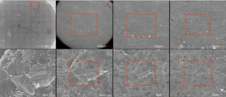
particular zones of the pellet, called hereafter “Region Of Interest” (ROI) were selected. Images of these zones were recorded at different magnifications prior the dissolution test, in order to find “easily” the ROI after the dissolution steps (Fig. 1).
2.2. Methods
2.2.1. Dissolution of sample
The pellet was put in contact with 25 mL of 0.1 M HNO3solution at
60 °C under stirring in a PTFE dissolution reactor. At regular intervals, the sample was removed from the dissolution device, washed with water three times and finally the excess of water was removed with an absorbent paper, in order to stop the dissolution process. Then, the sample was introduced in the ESEM chamber equipped with a Peltier stage. The Peltier stage was cooled down to 2 °C prior the introduction of the sample introduction. A great caution was paid to the pumping sequence in order to avoid any dehydration of the sample. This pumping sequence consisted in 8 differential pumping steps between 500 and 750 Pa of H2O. Finally, the water vapor pressure in the
chamber was adjusted to 300 Pa which corresponded to a relative hu-midity of 42.5%. With this experimental procedure, the sample was never dried. The use of the ESEM under wet conditions prevented the dissolution experiment from perturbations induced by the sample ob-servation.
After recovering the region of interest and recording the image series, the sample was put again in contact with the solution. This se-quence was repeated several times up to the end of the dissolution test. Thus, the full experiment corresponded to a multistep observation se-quence.
2.2.2. Recording of ESEM images
The ESEM used during this study was a Quanta 200 ESEM FEG (commercialized by the FEI Company). After the sample was introduced in the ESEM chamber, the images were recorded using a specific gas-eous secondary electron detector [19]. The imaging conditions were defined in order to reduce the consequences of irradiation of the sample by the electron beam [20,21]. Indeed, the irradiation of the sample could have strongly modified locally the reactivity of the sample surface and finally generated unexpected local modifications of the dissolution process (i.e. increase or decrease of the local dissolution kinetics). Thus, this effect had to be avoided - or limited - as much as possible. The optimized imaging conditions (that are optimized for the Quanta 200 ESEM FEG used in this study) are the following:
o Working distance = 6 mm o E0= 6 kV
Fig. 1. Series of images recorded at different magnifications prior the dissolution test that are used to find the same Region Of Interest (ROI) from one dissolution
o Spot size = 3–4
o Diaphragm diameter = 20 μm o Image acquisition conditions
▪2048 × 1887 pixels ▪1 μs per pixel
▪Accumulation of 16 images with drift correction
o Magnification = 20,000, 10,000, 5000 times (corresponding to {6.35 μm; 5.48184 μm}, {12.7 μm; 10.9737 μm} and {25.4 μm; 21.9273 μm} field of views respectively)
o The images were recorded with tilt angles corresponding to −10°, 0° and 10°.
The image recording conditions resulted from a compromise be-tween the final image quality required to reconstruct the sample surface (in terms of signal/noise ratio and limitation of the image deformation) and the irradiation of the sample surface by the electron beam (no observable sample surface modification of the ROI compared to the other parts of the sample).
2.2.3. 3D-SEM surface image reconstruction and height map
The tilted image series were pre-aligned using Fiji software and the particular SIFT method [22]. The image surface reconstructions were performed using the commercial Alicona Mex software with the three images recorded at the same magnification [23] (Fig. 2a, b, c). Then the image of the sample surface was calculated, the 3D image was aligned by comparison with a reference plane which was the plane cutting the image in two parts with the same quantity of matter on the top and on the bottom sides (Fig. 2d). Thus, 16 bits images were extracted from the 3D surface reconstructions using a scale of 1 Å per pixel (corresponding to the grey scale). In these conditions, the maximum assessable scale was 6.5535 μm (Fig. 2e). Obviously, this scale must be modified and adapted by adjusting the length associated to a pixel, depending on the size of the studied sample. These images (hereafter called “height maps”) contain the coordinates of each point of the sample surface in a three dimensional Cartesian system. They are the raw material that will be used to characterize the topographic changes of the surface sample as a function of the dissolution time.
2.2.4. Atomic Force Microscopy (AFM)
The sample was also characterized by Atomic Force Microscopy using a MULTIMODE 8 AFM apparatus (with a lateral resolution of approximately 8 nm and an optimal z resolution of 1 Å) equipped with a Nanoscope 5 controller from Bruker Germany. The observed sample
was put in contact with the dissolution medium for 1064 h prior the microscopic characterization. The same Region of Interest (ROI) was also observed by ESEM before and after AFM.
AFM imaging was performed in the peak force mode, under dry conditions using SNL tips (silicon tip on silicon nitride cantilever) from Bruker Company with a spring constant of 0.24 N·m−1. This mode has
been used with specific parameters defined by the operator in order to minimize the force and to use the same tip for all the samples. Furthermore, the peak force mode has been used in order to minimize the energy that is dissipated at the sample surface during the AFM image recording with respect to their fragility (thin hydrated layers probably covers the sample). Last, a 16 bits height map with a 0.4 Å per pixel resolution was also extracted from the AFM topographic image.
3. Validation of the height maps
3.1. Mex height map versus AFM height map
The same region of interest (ROI) of the sample surface was ob-served using two types of microscopies (Fig. 3b and d) in order to compare both datasets and to validate the height values obtained with Mex by comparison with the AFM measurements.
The main difference between both techniques was the time required to record an image of the ROI. Concerning AFM, one day was necessary to recover the ROI (i.e. a 10 μm × 10 μm zone on a pellet of 5 mm in diameter with marks). Then, the time necessary to record an image with the desired resolution was 1.5 h. The precision in the height values was approximately 1 nm. Regarding the surface reconstruction, finding the ROI and recording the ESEM image series required 20 min for the 3 different magnifications. Then, it took 15 min to reconstruct the topo-graphic image of the surface using the Mex software. The precision in the determination of the height values was approximately 30–40 nm (the determination of this value will be detailed later).
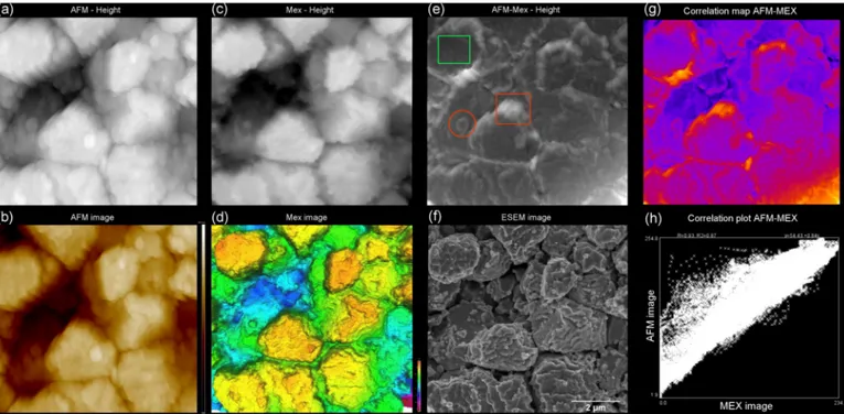
The height maps extracted from the Mex reconstruction and the AFM image were thus compared. Since AFM technique provided the most accurate measurements of the surface sample heights, these values were used to determine the correctness of the heights retrieved using the Mex software. Thus, the AFM height map was used as a reference to describe the real sample surface. Both AFM and Mex height maps of the same ROI (with the same scale) are reported inFig. 3a and c and the image showing the difference between AFM and Mex height maps is reported inFig. 3e. A more accurate comparison of both images was obtained by plotting the correlation map (Fig. 3h) between both images and by determining the cross-correlation coefficient [24]. In this case, the figure of merit (R2) was equal to 0.85. This value reflects the very
good correlation between the two height maps but also the defects present in both images and that are inherent to each type of char-acterization technique. The correlation map showed the defects of the AFM image as well as those of the Mex image.
The usual artifacts were observed on AFM images obtained on samples with large topography:
- The image of the AFM tip was observed on the steep edges of the grains. This defect was highlighted inFig. 3e by a red rectangle in the image difference between AFM and Mex height maps and re-ferenced as Zone 1 inFig. 4a.
- The deformation of the image arising from the high radius of cur-vature of the tip used relative to the geometry of the feature to be imaged (apparent increase of the sample size called tip artifact) [25]. This defect was highlighted inFig. 3e by a red circle on the image difference between AFM and Mex height maps and referenced as Zone 2 inFig. 4a.
Artifacts of Mex images due to the reconstruction process were also observed:
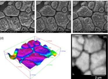
Fig. 2. Tilted image series {−10°; 0; 10°} of the same zone of the sample (a, b,
c) leading to the 3D surface image reconstruction using Alicona Mex software (d) and the corresponding extracted 16 bits height map (e). The features of the grains are recognizable on the 3 different representations of the surface.
- The main one corresponded to the limit of the reconstruction re-solution along the z-axis (estimated to 30–40 nm) which can be seen on the difference image on the top of the grains (shown by a red rectangle onFig. 3e). There is much more topographic information at the nanometer scale on the AFM image than in the Mex image. - The general deviation of the baseline (that remained limited on this
example, but still visible on the correlation map –Fig. 3g). It was related with a discrepancy of the reference planes between both height maps.
At this stage, the direct comparison between Mex and AFM height maps revealed a very good agreement between both datasets. This agreed with the conclusions of Raspanti et al. who showed the excellent visual match between Mex and AFM height maps recorded on biological materials [26].
In addition, profiles were drawn at the same location using both AFM and Mex height maps. The data and the position of the profiles on the selected ROI are reported inFig. 4. Using these data, the accuracy of the Mex height values was determined by comparison with the AFM height values. The procedure used is described hereafter. First, the height difference between two points of the Mex profile was measured (HDMex). Second, the height difference between the same points was
measured from the AFM height profile (HDAFM) (Fig. 4a). Third, the
percentage of height difference between AFM and Mex measurements was determined as follows:
= ×
%HD 100 ((HDMex HDAFM)/HDAFM) (1)
The %HD value is the relative difference between Mex reconstruc-tion and AFM data.
This procedure was repeated several times on this profile in order to determine the %HD values for several HDAFMvalues. This set-up was
also applied on four other profiles determined from the same AFM and Mex height maps. The obtained %HD values are reported as a function of the height difference determined using the AFM image, HDAFM, in
Fig. 5a whereas the absolute values of the difference │HDMex− HDAFM│are plotted versus the height difference determined
using the AFM image, HDAFM, inFig. 5b. This dataset allowed
de-termining the accuracy of the height values measured from the Mex reconstructed image as a function of the height difference. As an ex-ample, when the height difference between two details was equal to 30 nm, the accuracy reached ± 60%. The accuracy equaled ± 20% and 5% when the height difference was 130 nm and 1500 nm, respectively. In the conditions used for the present study, the average height dif-ference between the HDMexand HDAFMmeasurements was 38 nm. This
value is represented by the dashed line inFig. 5b. It corresponds to the resolution of the Mex image in the height direction.
As a conclusion, there was a good accuracy of the relative z posi-tions determined as well as the {x,y} coordinates (depending on the initial SEM image magnification). This result indicates that the image was not significantly deformed by the 3D surface reconstruction process Fig. 3. Validation of the Alicona Mex surface reconstructions. Observation of the sample surface using several types of microscopies: (a) AFM height map; (b) AFM
view of the sample; (c) Mex height map (using the same scale for the z pixel than for AFM height map); (d) 3D Mex reconstruction; (e) image of difference between AFM and Mex height maps; (f) SEM image; (g) correlation map between AFM and MEX height maps and (h) correlation plot between AFM and MEX height maps. (It must be noted that the ratio between the contrast and the brightness of the “Image of difference between AFM and Mex height maps” was enhanced in order to highlight the differences). (For interpretation of the references to color in this figure, the reader is referred to the web version of this article.)
Fig. 4. Height profiles of the same zone (a) extracted from the Mex height map
(b) and AFM height map (c). The size of the images was 7.73 μm × 8.26 μm. The HDMexand HDAFMvalues corresponded to the height differences measured
using the Mex software. This conclusion is also in good agreement with the results already reported in the literature [26].
3.2. Mex height maps recorded at different magnifications
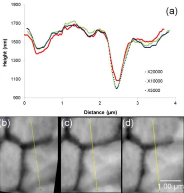
Height maps of the same region of interest were reconstructed with Mex software at several magnifications. Three profiles determined on the same zone and the corresponding images are reported inFig. 6a. The width of the line (integration zone) was adjusted as a function of the image magnification and it always corresponded to 33 nm (Fig. 6b, c, d).
A general good agreement between the three reported profiles was observed. On the basis ofFig. 6a, the baseline of the profile obtained from the image reconstructed at 20 kX was slightly shifted compared to the profiles obtained at 5 and 10 kX. This discrepancy was attributed to the automatic determination of the reference plane by the Mex soft-ware. Indeed, the image obtained after the reconstruction process could be tilted and straightened with respect to a reference plane. In this case, the reference plane was fixed in order to set one half of the volume below the plane and the second half of the volume under the plane. As a consequence, this plane was not necessarily the same for the two images (containing the same ROI) recorded at different magnifications. Thus, this yielded to a slight shift of the baselines for the profiles re-ported inFig. 6a.
Another discrepancy was observed at the position of the grain boundary. The depth of the grain boundary measured from the 5 kX and 10 kX reconstructed images was higher than that obtained from the 20 kX 3D reconstruction. It probably corresponded to the presence of a crystallite that was not always exactly positioned at the same location
depending on the magnification of the SEM image series. Nevertheless, the very good agreement between the 3 sets of data can also be con-sidered as a proof of the quality of the surface reconstructions.
4. How to use the height map series?
4.1. Height maps coupled with SEM images
From the 3D surface reconstructions, the surface area of the solid/ solution interface was determined precisely. Thus, this method allowed calculating this parameter in the case of materials presenting low spe-cific surface area that were not accessible by the usual techniques such as BET method using Kr adsorption. In addition, using stack of 3D re-constructions allowed monitoring of the evolution of the surface area of the sample during dissolution.
The Abbott-Firestone curve (or Bearing Area Curve) was used to describe the surface texture of the sample (for more details, please refer to Fig. 4reported by Loberg et al. [27]). From this curve, several parameters of interest for the kinetics of local dissolution processes were determined [28]:
o Core void volume (Vvc) expressed in cm3·m−2
o Core material volume (Vmc) expressed in cm3·m−2
o Valley void volume (Vvv) expressed in cm3·m−2
o Height of the core material (Sk) expressed in μm
By considering that the surface of the sample was flat before the dissolution test, the value of Vvcdirectly represented the quantity of
matter that was dissolved (assuming that the highest points of the re-constructed surface where included in the initial surface of the sample) (Fig. 7).
Fig. 5. Determination of the accuracy of the Mex height values. (a) Relative
height difference (%HD) measured between Mex and AFM data at the same (x, y) coordinates and (b) absolute values of the height differences between Mex and AFM measurements (│HDMex− HDAFM│). The line reported in (b)
re-presents the average value of all the height differences measured (i.e. 38 nm).
Fig. 6. (a) Height profiles determined on the same ROI using Mex
3D-re-constructions of SEM images recorded at different magnifications; (b) height map and corresponding profile reconstructed from ×20,000 magnification SEM images (line integration on 10 pixels); (c) height map and corresponding profile reconstructed from ×10,000 magnification SEM images (line integration on 5 pixels); (d) height map and corresponding profile reconstructed from ×5000 magnification SEM images (line integration on 3 pixels). NB: The width of the integration line was adjusted as a function of the magnification and corre-sponded to 33 nm. The size of the images reached 2.82 μm × 3.78 μm.
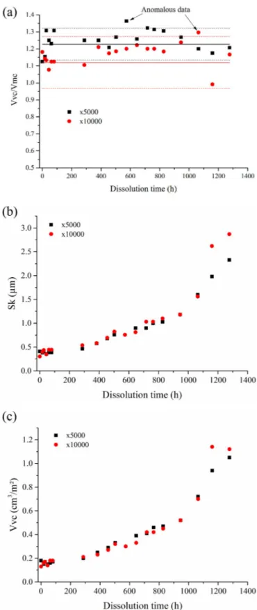
The evolution of the parameters associated with Abbott-Firestone curve extracted from the 3D reconstructions of the solid/solution inter-face of the sample during dissolution is reported inFig. 8. First, the ratio between the core void volume (Vvc) and the core material volume (Vmc)
was plotted for the stack of 3D reconstructions in order to detect anomalous reconstructions. FromFig. 8a, it appeared that the ratio be-tween the volume of matter and the core void volume of the re-construction was independent of the dissolution times, but slightly de-pendent on the magnification (i.e. the dimensions of the reconstructed zone). The average value and associated standard deviation of the ratio was 1.23 ± 0.09 and 1.12 ± 0.15 at ×5000 and ×10,000, respec-tively. The anomalous data that are evidenced fromFig. 8a correspond to images where detached grains are deposited on the sample surface. The evolution of the height of the core material and the void volume of the core are plotted inFig. 8b and c, respectively. Sk and VVCwere found to
increase with the dissolution time. This result showed that the depth of the “valleys” dug during the dissolution of the pellet increased. This was a strong indication that the dissolution did not occur by normal retreat of the surface, which would lead to constant Sk and Vvcvalues.
4.2. Height map series
During the study of the dissolution of materials, several re-constructions of the same ROI were obtained for various different dis-solution times. As explained before, a height map was extracted for each reconstruction (where one grey level corresponds to 1 Å). Thus, these height maps were combined together into a stack. The images of the stack were aligned twice using alternatively the “Linear Stack Alignment with SIFT” [22] and the “StackReg” plugins with Fiji soft-ware [29]. One limit of this technique was the absence of invariant points during the dissolution process allowing an accurate alignment of all the images in the z direction, and thus the evaluation of the absolute dissolved volumes. However, this limit was overcome by considering one detail that remained recognizable from one image to the next one. Even if the error was not determined precisely, it was considered to remain relatively low (few nanometers to ten nanometers from one image to the next one).
The aligned stack of images offered the possibility to describe quantitatively the dissolution process at the surface of the material as a function of time, with images that were spatially resolved in the 3 di-rections.
Fig. 7. Abbott-Firestone curve and associated parameters considered to
char-acterize the sample texture.
Fig. 8. Evolution of the parameters associated to the Abbott-Firestone curve
determined from the 3D reconstruction of the topography of the sample during dissolution: (a) ratio between core void volume and core material volume (detection of anomalous reconstruction); (b) height of the core material; (c) core void volume used to calculate the amount of dissolved material.
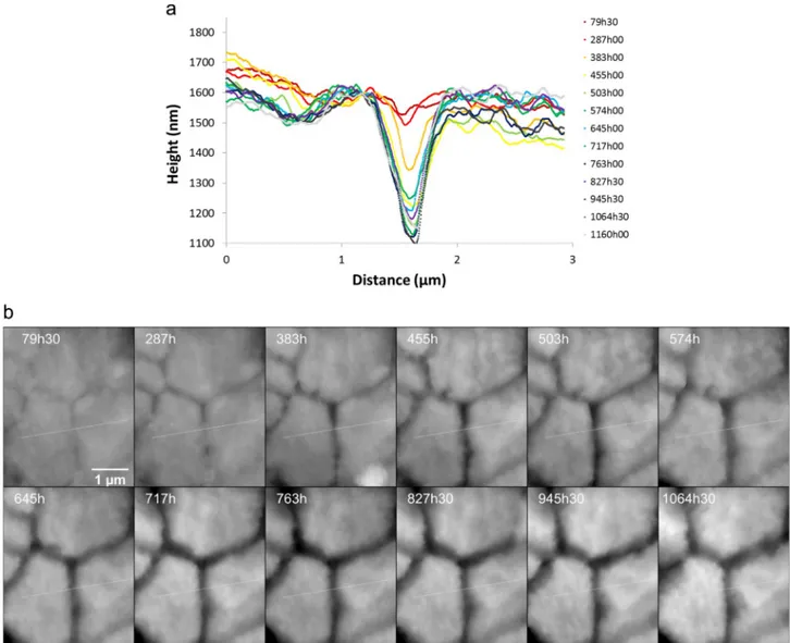
4.3. Profiles in the height map series
Profiles in the height map series were drawn to quantify the local height variations as a function of the dissolution time. Two profiles were extracted from the stacks of images recorded with various mag-nifications (Fig. 9). The profiles reported inFig. 9a and c correspond to 20 kX and 5 kX height map image series, respectively. They were aligned in order to keep the position of one point (point I) invariant in height with the dissolution time. From the high magnification images stack (Fig. 9a), the preferential dissolution at the grain boundaries was clearly evidenced. This preferential dissolution both corresponded to the increase of the depth and of the width of the grain boundary. From the low magnification images stack (Fig. 9c), the detachment of grains during the dissolution process was clearly evidenced. It corresponded to the fast depth modifications that were observed from one time to the next one.
The whole (or part of the) profile was integrated on a selected width of matter corresponding to the width of the line used to extract the profile. Thus local quantities of matter removed during the dissolution/ corrosion process were determined accurately. Using the data from the whole image series, the dissolution rates were evaluated at the micro-scopic scale.
4.4. Differences of height maps
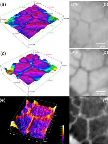
The determination of differences of height maps can be useful to locate the zones of the sample where the dissolution process was pre-dominant. This first required to reconstruct 3D images of the same zone at two different dissolution times and then to extract height maps. The difference between two aligned height maps was calculated using the Fiji software. The result was an image highlighting the preferential dissolution/corrosion zones at the surface of the material. Reconstructed surfaces after 287 h and 645 h of dissolution are reported inFig. 10a and c, respectively, whereas the corresponding height maps are reported inFig. 10b and d, respectively, and the difference map is shown inFig. 10e (3D view) andFig. 10f. FromFig. 10f, it is clear that a preferential dissolution occurred at the grain boundaries and at the triple junctions of the ceramic. As the x-, y- and z-scales were expressed in metric units, it was possible to derive the quantity of matter that was dissolved locally between 287 h and 645 h of dissolution.
The main limit of the comparison of two images obtained by 3D reconstruction method from SEM images was the necessity to have a reference plane, or “reference points”, which remained at the same location in both images. In other words, this implies that a zone of the sample remained unaffected by the dissolution process. In the studies
already reported, authors used a shadowing method to hinder the contact of the corrosive liquid with the sample in a specific zone. As example, platinum masks could be incorporated in the sample prior the dissolution test [30], a part of the sample could be protected with a coating [10] that could not be dissolved or a particular assembly jig could be used to create a non-wetted reference zone [9,31]. However, these techniques require to record large sized 3D images of the sample (from few hundreds of micrometers to millimeter scale) and they are impossible to implement with the reconstruction method reported herein (as the final image size only represents few square micrometers). As a consequence, when the dissolution mechanism occurred by normal retreat of the surface (i.e. general decrease of the sample thickness), no reference points were found on both images and the quantity of dis-solved matter was not accurately determined. This limit was probably overcome by implementing reference points (or reference plane) in the sample that would remain unaltered during the dissolution experiment. This will be part of future technical developments.
More generally, if the dissolution process is not too fast, some un-altered zones could be found despite the dissolution progress. These invariant points could be used to align the different height maps by assigning the same absolute height (i.e. grey level) in both height maps.
5. Conclusions
An accurate method for the characterization of materials dissolution at the micrometric scale was reported. This method was based on (E) SEM tilted image series of the same zone at the sample surface after several exposition times to a corrosive solution. After each observation, a 3D surface reconstruction was obtained and these topographic images were compared to AFM images in order to validate the height values obtained. The quality of the 3D reconstruction from (E)SEM images was close to the AFM image one as the figure of merit of the correlation map between both images reached 0.85.
The main advantages of this characterization technique are the high quality of the 3D surface reconstructions, the fast acquisition of the data, the possibility to observe wet samples (by using an Environmental Scanning Electron Microscope) and the limited beam effects. This technique can be applied to the observation of topographic changes occurring at the surface of numerous materials due to various me-chanisms such as dissolution and corrosion, formation of coatings or corrosion layers, cracking under mechanical stress… It could be also extended to the observation of high temperature transformations such as glass-ceramic crystallization, grain sintering, grain growth, etc. Fig. 9. (continued)
References
[1] J.-H. Hsu, J. Bai, C.-W. Kim, R.K. Brow, J. Szabo, A. Zervos, The effects of crys-tallization and residual glass on the chemical durability of iron phosphate waste forms containing 40 wt% of a high MoO3Collins-CLT waste, J. Nucl. Mater. 500
(2018) 373–380,https://doi.org/10.1016/j.jnucmat.2018.01.005.
[2] D. Horlait, F. Tocino, L. Claparède, N. Clavier, J. Ravaux, S. Szenknect, R. Podor, N. Dacheux, Environmental SEM monitoring of Ce1−xLnxO2−x/2mixed oxides
mi-crostructural evolution during dissolution, J. Mater. Chem. A 2 (2014) 5193–5203,
https://doi.org/10.1039/C3TA14623E.
[3] T. Cordara, S. Szenknect, L. Claparede, R. Podor, A. Mesbah, C. Lavalette, N. Dacheux, Kinetics of dissolution of UO2in nitric acid solutions: a
multi-parametric study of the non-catalysed reaction, J. Nucl. Mater. 496 (2017) 251–264,https://doi.org/10.1016/j.jnucmat.2017.09.038.
[4] S. Szenknect, S. Finkeldei, F. Brandt, J. Ravaux, M. Odorico, R. Podor, J. Lautru, N. Dacheux, D. Bosbach, Monitoring the microstructural evolution of Nd2Zr2O7
pyrochlore during dissolution at 90 °C in 4 M HCl: implications regarding the evaluation of the chemical durability, J. Nucl. Mater. 496 (2017) 97–108,https:// doi.org/10.1016/j.jnucmat.2017.09.029.
[5] D. Dalmas, A. Lelarge, D. Vandembroucq, Quantitative AFM analysis of phase se-parated borosilicate glass surfaces, J. Non-Cryst. Solids 353 (2007) 4672–4680,
https://doi.org/10.1016/j.jnoncrysol.2007.07.005.
[6] M. Urosevic, C. Rodriguez-Navarro, C.V. Putnis, C. Cardell, A. Putnis, E. Ruiz-Agudo, In situ nanoscale observations of the dissolution of {10-14} dolomite clea-vage surfaces, Geochim. Cosmochim. Acta 80 (2012) 1–13,https://doi.org/10. 1016/j.gca.2011.11.036.
[7] A. Damian, F. Maroun, P. Allongue, Electrochemical de-alloying in two dimensions: role of the local atomic environment, Nanoscale 8 (2016) 13985–13996,https:// doi.org/10.1039/C6NR01390B.
[8] A. Luttge, U. Winkler, A.C. Lasaga, Interferometric study of the dolomite dissolu-tion: a new conceptual model for mineral dissolution, Geochim. Cosmochim. Acta 67 (2003) 1099–1116,https://doi.org/10.1016/S0016-7037(02)00914-6. [9] D. Daval, R. Hellmann, G.D. Saldi, R. Wirth, K.G. Knauss, Linking nm-scale
mea-surements of the anisotropy of silicate surface reactivity to macroscopic dissolution rate laws: new insights based on diopside, Geochim. Cosmochim. Acta 107 (2013) 121–134,https://doi.org/10.1016/j.gca.2012.12.045.
[10] C. Fischer, S. Finkeldei, F. Brandt, D. Bosbach, A. Luttge, Direct measurement of surface dissolution rates in potential nuclear waste forms: the example of pyro-chlore, ACS Appl. Mater. Interfaces 7 (2015) 17857–17865,https://doi.org/10. 1021/acsami.5b04281.
[11] T.P. Weihs, Z. Nawaz, S.P. Jarvis, J.B. Pethica, Limits of imaging resolution for atomic force microscopy of molecules, Appl. Phys. Lett. 59 (1992) 3536–3538,
https://doi.org/10.1063/1.105649.
[12] S. Santos, V. Barcons, H.K. Christenson, J. Font, N.H. Thomson, The intrinsic re-solution limit in the atomic force microscope: implications for heights of nano-scale features, PLoS ONE 6 (2011) e23821, ,https://doi.org/10.1371/journal.pone. 0023821.
[13] R.S. Arvidson, C. Fischer, D.S. Sawyer, G.D. Scott, D. Natelson, A. Lüttge, Lateral resolution enhancement of vertical scanning interferometry by sub-pixel sampling, Microsc. Microanal. 20 (2014) 90–98,https://doi.org/10.1017/
S1431927613013822.
[14] M. Eulitz, G. Reiss, 3D reconstruction of SEM images by use of optical photo-grammetry software, J. Struct. Biol. 191 (2015) 190–196,https://doi.org/10.1016/ j.jsb.2015.06.010.
[15] A.P. Tafti, A.B. Kirkpatrick, Z. Alavi, H.A. Owen, Z. Yu, Recent advances in 3D SEM surface reconstruction, Micron 78 (2015) 54–66,https://doi.org/10.1016/j.micron. 2015.07.005.
[16] L.C. Gontard, J.D. López-Castro, L. González-Rovira, J.M. Vázquez-Martínez, F.M. Varela-Feria, M. Marcos, J.J. Calvino, Assessment of engineered surfaces roughness by high-resolution 3D SEM photogrammetry, Ultramicroscopy 177 (2017) 106–114,https://doi.org/10.1016/j.ultramic.2017.03.007.
[17] Q. Shi, S. Roux, F. Latourte, F. Hild, D. Loisnard, N. Brynaert, Measuring topo-graphies from conventional SEM acquisitions, Ultramicroscopy 191 (2018) 18–33,
https://doi.org/10.1016/j.ultramic.2018.04.006.
[18] C. Mignot, Color (and 3D) for scanning electron microscopy, Micros. Today 5 (2018) 12–17,https://doi.org/10.1017/S1551929518000482.
[19] D.J. Stokes, Principles and Practice of Variable Pressure/Environmental Scanning Electron Microscopy (VP-ESEM), John Wiley & Sons, Chichester, UK, 2008. [20] C.P. Royall, B.L. Thiel, A.M. Donald, Radiation damage of water in environmental
scanning electron microscopy, J. Microsc. 204 (2001) 185–195,https://doi.org/10. 1046/j.1365-2818.2001.00948.x.
[21] R.F. Egerton, P. Li, M. Malac, Radiation damage in the TEM and SEM, Micron 35 (2004) 399–409,https://doi.org/10.1016/j.micron.2004.02.003.
[22] D. Lowe, Distinctive image features from scale invariant keypoints, Int. J. Comput. Vis. 06 (2004) 91–110https://link.springer.com/article/10.1023/B:VISI. 0000029664.99615.94.
[23] MeX | Alicona - high-resolution optical 3D measurement,https://www.alicona. com/en/products/mex/.
[24] G. Chinga, K. Syverud, Quantification of paper mass distributions within local picking areas, Nord. Pulp Pap. Res. J. 22 (2007) 441–446,https://doi.org/10.3183/ npprj-2007-22-04-p441-446.
[25] C. Canale, B. Torre, D. Ricci, P.C. Braga, Recognizing and avoiding artifacts in atomic force microscopy imaging, Methods Mol. Biol. 736 (2011) 31–43,https:// doi.org/10.1007/978-1-61779-105-5_3.
[26] M. Raspanti, E. Binaghi, I. Gallo, A. Manelli, A vision-based, 3D reconstruction technique for scanning electron microscopy: direct comparison with atomic force microscopy, Microsc. Res. Tech. 67 (2005) 1–7,https://doi.org/10.1002/jemt. 20176.
[27] J. Loberg, I. Mattisson, S. Hansson, E. Ahlberg, Characterisation of titanium dental implants I: critical assessment of surface roughness parameters, Open Biomater. Sci. J. 2 (2010) 18–35https://benthamopen.com/FULLTEXT/TOBIOMTJ-2-18. [28] L.A. Franco, A. Sinatora, 3D surface parameters (ISO 25178-2): actual meaning of
Spk and its relationship to Vmp, Precis. Eng. 40 (2015) 106–111,https://doi.org/ 10.1016/j.precisioneng.2014.10.011.
[29] Stackreg plugin with Fiji software,http://bigwww.epfl.ch/thevenaz/stackreg/. [30] J.A. Taillon, C. Pellegrinelli, Y.-L. Huang, E.D. Wachsman, L.G. Salamanca-Riba,
Improving microstructural quantification in FIB/SEM nanotomography, Ultramicroscopy 184 (2018) 24–38,https://doi.org/10.1016/j.ultramic.2017.07. 017.
[31] M. Pollet-Villard, D. Daval, P. Ackerer, G.D. Saldi, K.G. Knauss, B. Wild, B. Fritz, Experimental study of dissolution kinetics of K-feldspar as a function of crystal structure anisotropy under hydrothermal conditions, Procedia Earth Planet. Sci. 17 (2017) 165–168,https://doi.org/10.1016/j.proeps.2016.12.042.
Fig. 10. Difference of height maps. 3D reconstruction of the solid/solution
in-terface after 645 h (a) and 287 h (c) of dissolution; corresponding height maps (z-scale: 1 pixel = 0.1 nm) obtained using the Fiji software ((b) and (d), re-spectively) and 3D (e) and 2D (f) views of the difference of height maps ob-tained between 287 and 645 h.