A Note on the Impact of Portfolio Overlapping in Tests of the Fama and French Three-Factor Model

W

ORKING

P

APERS

SES

F

S

E

S

W

-

S

F

U

F

| U

F

11.2012

N° 433

A Note on the Impact of Portfolio

Overlapping in Tests of the Fama

and French Three-Factor Model

A Note on the Impact of Portfolio Overlapping in

Tests of the Fama and French Three-Factor Model

Martin Wallmeier / Kathrin Tauscher

First draft, October 2012

Abstract

In the three-factor model of Fama and French (1993), portfolio returns are explained by the factors Small Minus Big ( ) and High Minus Low ( ) which capture returns related to firm capitalization () and the book-to-market ratio ( ). In the standard approach of the model, both the test portfolios and the factor portfolios   and   are formed on the basis of  and  . This gives rise to a potential overlapping bias in the time-series regressions. Based on a resampling method and the split sample approach already proposed by Fama and French (1993), we provide an in-depth analysis of the effect of overlapping for a broad sample of European stocks. We find that the overlapping bias is non-negligible, contrary to what seems to be general opinion. As a consequence, the standard approach of applying the three-factor model tends to overestimate the ability of the model to explain the cross-section of stock returns.

JEL classification: G12; G14

Keywords: Asset pricing; three-factor model; portfolio overlapping; size effect; value pre-mium.

∗_{Prof. Dr. Martin Wallmeier (corresponding author), Kathrin Tauscher, Department of Finance and}

Account-ing, University of Fribourg / Switzerland, Bd. de Pérolles 90, CH-1700 Fribourg, martin.wallmeier@unifr.ch, kathrin.tauscher@unifr.ch

1 Introduction 2

1

Introduction

The Fama and French three-factor model has long been established as one of the most widely accepted asset pricing models.1 It is based on two foundations: (i) the finding of Fama and French (1992) (in the following FF92) that the two variables  and book-to-market equity ( ) explain the cross-sectional variation of average stock returns, and (ii) the finding of Fama and French (1993) (in the following FF93) that mimicking factors for returns related to  and  explain a significant part of return variation over time. The mimicking factors introduced by Fama and French are known as Small Minus Big ( ) and High Minus Low ( ). Using  ,   and a market proxy as explanatory variables, FF93 run time-series regressions for 25 portfolios sorted on  and  . The intercepts are all close to zero, which indicates that the three factors “seem to do a good job explaining the cross-section of average stock returns.”2

A peculiar characteristic of the time-series regression setup in FF93 is that the sorting variables are the same for both the dependent and independent variables. FF93 remark:

“In the time-series regressions for stocks, the dependent returns and the two explana-tory returns   and   are portfolios formed on size and book-to-market eq-uity. Many readers worry that the apparent explanatory power of   and   is spurious, induced by the regression setup.”3

However, the authors argue:

“We think this is unlikely, given that the dependent returns are based on much finer size and   sorts (25 portfolios) than the   and   returns.”4

In fact, an independent test of FF93 supports this view. The idea of the test is to use two disjoint groups of stocks to measure the independent and dependent variables separately, thus

1 _{See, e.g., Bauer et al. (2010), p. 171: “Our test assets are 25 portfolios formed on size and B/M, which have}

become standard in asset pricing tests after the failure of CAPM”.

2

Fama and French (1993), p. 5.

3

Fama and French (1993), p. 46f. Similarly in Fama and French (1996), p. 76: “It may not be surprising, however, that portfolios like SMB and HML that are formed on size and BE/ME can explain the returns on other portfolios formed on size and BE/ME (albeit with a finer grid).”

4 _{Fama and French (1993), p. 47. The authors denote book-to-market equity by   instead of  in}

1 Introduction 3 excluding any overlap. Further support for the three-factor model comes from results based on different sorting variables for the test portfolios (see FF93, p. 47ff; Fama and French (1996)). By and large, the U.S.-results of FF92 for  and  as determinants of expected returns have been confirmed for other markets, including Asia Pacific, Japan, and European countries.5 There is less international evidence, however, on the validity of the risk-based interpretation of FF93. In many countries, the time series regressions are more difficult to replicate due to a substantially smaller number of stocks available. For this reason, Ziegler et al. (2007) and Schrimpf et al. (2007), e.g., use a (4x4)-classification of  and  for German stocks in contrast to the (5x5)-classification of FF93. Thus, the portfolios get closer to the (2x3)-building blocks of   and  , leading to a higher similarity between independent and dependent variables. The independent test of FF93 is also not availabe if the number of stocks is too small for a split into two disjoint groups. Thus, the impact of portfolio overlaps might be more important in these markets than in the U.S.

We are not aware of any direct evidence on the impact of portfolio overlaps in applications of the three-factor model. Some authors mention that results remain basically the same when applying the independent FF93 test with disjoint groups.6 They tend to explain any remaining differences with the smaller number of stocks in the test portfolios after splitting the sample in two.7 In all, it seems to be generally accepted that overlapping does not significantly influence the empirical results in typical tests of the three-factor model. Our contribution is to provide an in-depth analysis of the impact of overlapping for a sample of European stocks. We show that the estimated coefficients of the time-series regressions for standard (5x5)-test portfolios are biased due to overlapping of dependent and independent variables. Portfolio overlapping is not the main driver of results for the three-factor model, but its impact is non-negligible. As a rough estimate for our sample, the range of slope coefficients for - and  -portfolios is more than one third higher than in a setup without portfolio overlap.

The paper proceeds as follows. In the next section, we illustrate the overlapping problem. We then replicate the standard analysis of the three-factor model for a comprehensive sample of

5 _{See, e.g., Fama and French (1998), Griffin (2002) and Fama and French (2012).} 6 _{See Fama and French (1993), p. 46f., and Guidi and Davis (2000), p. 10 f.} 7 _{See Guidi and Davis (2000), p. 11.}

2 The Portfolio Overlapping Problem 4 European stocks (Section 3). This analysis seems interesting in itself, because recently published studies for European countries provide different results (see Schrimpf et al. (2007) and Bauer et al. (2010)); however, our main motivation is to obtain a realistic data base for studying the overlapping problem. In line with expectations, the estimated slope coefficients of   and   are significantly different from zero and vary systematically with the  and  characteristics of the 25 test portfolios. To test our hypothesis that part of this variation is tautological, we randomly resample returns within the cross-section of our sample in such a way that any relationship of  and  with stock return is destroyed (Section 4). If   and   still appear to capture common components of return variation, this must be due to the overlapping of portfolios sorted on the basis of the same variables. We verify our results using estimations with disjoint samples for measuring the dependent and independent variables. Section 5 concludes with a discussion of practical implications of our results.

2

The Portfolio Overlapping Problem

The three-factor model of FF93 can be written as:

 = + 1 + 2 + 3 +  (1)

where  is the portfolio excess return in month ,   is the market excess return,  and

_  = 1     3 are regression coefficients and  is an error term. To compute   and

 , the sample stocks are divided into six portfolios, resulting from the intersection of two

 groups ( measured by market capitalization) and three  groups. We denote these portfolios by 11, 12, 13, 21, 22, 23, where  refers to the  group,  to the  group and the numbers are in ascending order of the variables. A return spread for portfolios of small minus big stocks is computed for each of the three  classes, and   is then

defined as the mean of these three spreads in month .8 Similarly,   is the mean return

spread of high minus low  stocks within the same  group.9 _{Each year, the cross-section}

8

  = [(11− 21) + (12− 22) + (13− 23)] 3 where  is the return in month  of

portfolio .

9 _{ }

2 The Portfolio Overlapping Problem 5 of stocks is also categorized into five quintile groups of  and  . The intersection of the independent  and  splits determines the composition of the 25 portfolios  for each of which Eq. (1) is estimated. These portfolios are denoted by 11     55 in the same logic as before, but with capital letters to indicate test portfolios. Due to the same sorting variables, the assignment of stocks to one of the 25 test portfolios is related to the assignment of this stock to one of the six components of   and  . For example, the stocks of test portfolio 11 will all be included in 11. Therefore, the return of 11 will tend to be positively related to   (which considers 11 with a positive sign) and negatively related to   (which considers 11 with a negative sign). Similarly, all stocks of test portfolio 55 will be part of 23, which induces negative and positive relations of this test portfolio’s return to   and  , respectively.

The inclusion of   can also have an influence on the slope coefficients of the market factor  . For illustration purposes only, let’s assume that the market return, in a capitalization-based weighting scheme, primarily reflects the return of blue chips, denoted by . Abstracting

from the specifics of  , we can simplify this factor to − , where  captures

the return of small caps. With these simplifications, Eq. (1) can be rewritten as:  = + 1+ 2(− ) + 3 + 

= +

¡

_{1− 2}¢+ 2+ 3 +  (2)

For a portfolio  of small capitalization stocks, we expect to find

• a significantly positive coefficient 2, because portfolios  and  overlap;

• a larger coefficient 1 compared to a one-factor model with only the market return

as explanatory variable, because the net market impact is now given by the difference ¡

_{1− 2}¢;

• an increase of the 2_{-coefficient compared to the one-factor market model, because the}

-factor is by construction related to and therefore adds to the explanatory power

3 Empirical Application of the Three-Factor Model 6 For portfolios  consisting of high capitalization stocks, we expect to find a strong relationship to the market factor (), while the additional overlapping effect introduced by the  and

  factors is supposed to be small. Thus 2 will be smaller than for small stock portfolios,

the coefficient _1 will be similar to the corresponding coefficient in the one-factor model, and the increase in the 2-coefficient compared to the one-factor model will be smaller than for small stock portfolios .

Finally, if substantial overlapping exists, the _3 coefficient will tend to increase when moving up to higher  portfolios within the same  class.

These relationships are actually present in the estimation results of Ziegler et al. (2007) for a German sample as well as Bauer et al. (2010) and Heston et al. (1999) for the European stock market.10 However, the contribution of portfolio overlapping is not identifiable. To clarify its role, we first present an empirical analysis for the European market similar to previous literature and then test for the impact of portfolio overlap.

3

Empirical Application of the Three-Factor Model

3.1

Prior Literature

Following the Fama and French studies of 1992 and 1993, a large body of literature has studied the determinants of risk and expected return in international asset markets. An important part of this research has focused on developing and testing conditional models which allow for time-varying risk premia.11 A related key aspect is the ongoing debate on whether the empirical determinants of expected returns are rather “anomalous” firm characteristics or risk factor sensitivities.12 We do not review this literature since our main interest lies on the specific overlapping aspect of standard tests of the three-factor model.

1 0 _{In Bauer et al. (2010), results for the one factor model are not available.}

1 1 _{See, e.g., Jagannathan and Wang (1996), Ferson and Harvey (1999), Hodrick and Zhang (2001), Lettau and}

Ludvigson (2001), Wu (2002), Wang (2003), Petkova and Zhang (2005), Zhang (2005), Avramov and Chordia (2006), Lewellen and Nagel (2006), Santos and Veronesi (2006), Ang and Chen (2007), Amman and Verhoven (2008) and Adrian and Franzoni (2009).

1 2 _{See, e.g., Daniel and Titman (1997), Berk (2000), Davis et al. (2000), Pastor and Stambaugh (2000) and Daniel}

3.2 Data and Descriptive Statistics 7 We limit our discussion to two prior papers to which our study is closely related. The first paper of Bauer et al. (2010) forms the basis for our empirical analysis in this section. Bauer et al. (2010) study conditional asset pricing models and stock market anomalies for a sample of about 2500 firms from 16 European countries over the time period from 1985 to 2002. We use a similar database for the more recent time period from 1989 to 2009 and adopt the same estimation approach while leaving out conditional models. Bauer et al. (2010) confirm the existence of the size effect but do not find a value premium: “The coefficient on size is negative and significant. Thus, a size effect is present in the cross-section of European stock returns [...]. The book-to-market coefficient is positive but insignificant, which means that the value premium is absent.” (p. 184) This finding is surprising, because it seems to be in contrast to recent U.S. studies which suggest a reversal of the size effect but confirm the value premium.13 It is also opposite to evidence of Schrimpf et al. (2007) for Germany over the period 1969 to 2002: “The ‘value premium’ can also be observed empirically on the German stock market” (p. 887), but “no negative relationship between size and average returns can be found for the German stock market. [...] One can even observe a tendency that average returns rise when size increases in our extended sample period” (p. 887f.)

This discrepancy of results for the German market and a comprehensive European sample shows that the dabate on return anomalies is still not settled. This is why the first empirical part of this study is of interest in itself, besides our focus on the overlapping problem.

3.2

Data and Descriptive Statistics

Our database from Thomson Reuters Datastream contains listed firms from 16 European coun-tries (Austria, Belgium, Denmark, Finland, France, Germany, Greece, Ireland, Italy, the Nether-lands, Norway, Portugal, Spain, Sweden, Switzerland, United Kingdom) over the period from December 1989 to December 2009. The sample includes failed companies to avoid a survivorship bias. Firm-years are included if the following data are available: the market capitalization in June of year  the book-to-market ratio ( ) in December of year  − 1 and monthly stock returns in year . Following Bauer et al. (2010), we require the  ratio to be non-negative.

3.2 Data and Descriptive Statistics 8 Starting with the largest market capitalization, firms are kept in the sample until a cumulated market capitalization of 85% in each country is reached. Thus, very small firms are excluded from the empirical analysis. We apply this selection rule on an annual basis. The final sample consists of 1945 firms. We convert local currency data into Euro using the respective exchange rates.

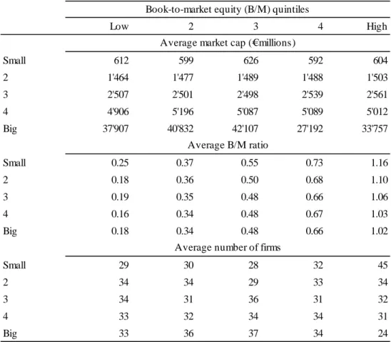
Following FF93, we form 25 - portfolios from independent quintile sorts based on market capitalization and  . The portfolio composition is updated at the end of June each year. Table 1 shows portfolio averages for the number of firms,  and  over all years of the sample period. The average number of firms varies between a minimum of 24 and a maximum of 45. By construction, the variation of  is strong across  quintiles, but small in the  dimension. Analogously,  varies strongly across the  quintiles, but is almost the same for different  groups within a given  quintile.

– Insert Table 1 (p. 22) about here. –

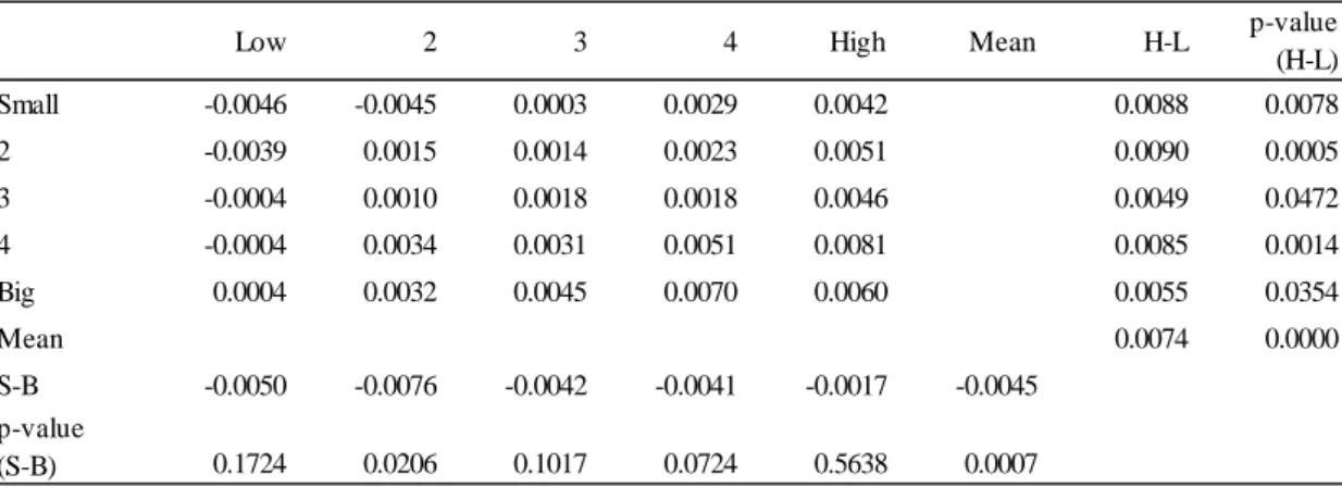
Table 2 reports average monthly excess returns of the 25 portfolios. To obtain excess returns, we subtract the three-month LIBOR rate from stock returns. The portfolios are value-weighted on the basis of the market capitalizations at the end of June and held constant for one year. Results show that portfolio returns tend to increase with  and . Portfolio (1,2) earns the smallest average return of -0.46% while portfolio (4,5) has the highest average return of 0.81%.14 The return differential between high  and low  portfolios (see column “H-L”) is always positive and statistically significant. On average, the spread is 0.74% per month, which means that firms in high  portfolios earn about 8.88% p.a. higher returns than firms in low  portfolios. Thus, we find evidence of a significant value premium in European markets. The return differences between small size and big size portfolios are all negative (see row “S-B”) indicating a negative size effect. Not all S-B spreads are significantly different from zero on the 5%-level, but on average, big stocks earned a statistically significant premium of 0.45% per month over small stocks.

1 4

The first portfolio number in brackets refers to the size group, the second to the  group (see Tables 1 and 2).

3.3 Time-Series Analysis 9

– Insert Table 2 (p. 23) about here. –

3.3

Time-Series Analysis

For each of the 25 portfolios defined in the last section, we estimate the three-factor model of Eq. (1) by running a time-series regression. We focus on the unconditional three-factor model assuming that the coefficients are constant over time. Our market proxy is the S&P 350 Europe Index. The factors   and   are defined as in FF93. Specifically, stocks are split into two groups (small and big) based on the median market capitalization at the end of June of each year. At the same time, stocks are ranked on the basis of  as of December of the previous year and allocated to three groups combining deciles 1 to 3 (low), deciles 4 to 7 (medium) and deciles 8 to 10 (high). From the intersections of the two  and three  groups, we construct six portfolios (small/low, small/medium, small/high, big/low, big/medium, big/high) and compute value-weighted monthly portfolio returns for the 12 months following portfolio formation.15   represents the difference between the simple average of

the small portfolio returns (small/low, small/medium, small/high) and the simple average of the big portfolio returns (big/low, big/medium, big/high) in month . Similarly,   is the

monthly difference between the simple average return of the high  portfolios (small/high, big/high) and the simple average return of the low  portfolios (small/low, high/low).

– Insert Figure 1 (p. 33) about here. –

Figure 1 illustrates the cumulative returns of  ,   and   over time.   returns hardly fluctuate in the sample period and remain slightly negative, which is in line with the observation in the last section that blue chip portfolios achieved higher returns than small firm portfolios. Cumulative   returns are largely positive and grow to almost 220% from July 1990 to December 2009, highlighting the profitability of a  based “value strategy” (long position in high  firms and short position in low  firms) in this period.

1 5

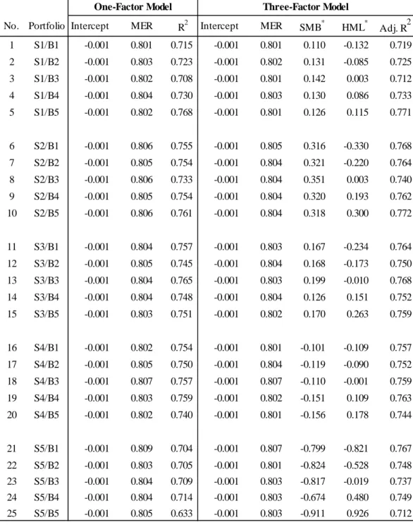
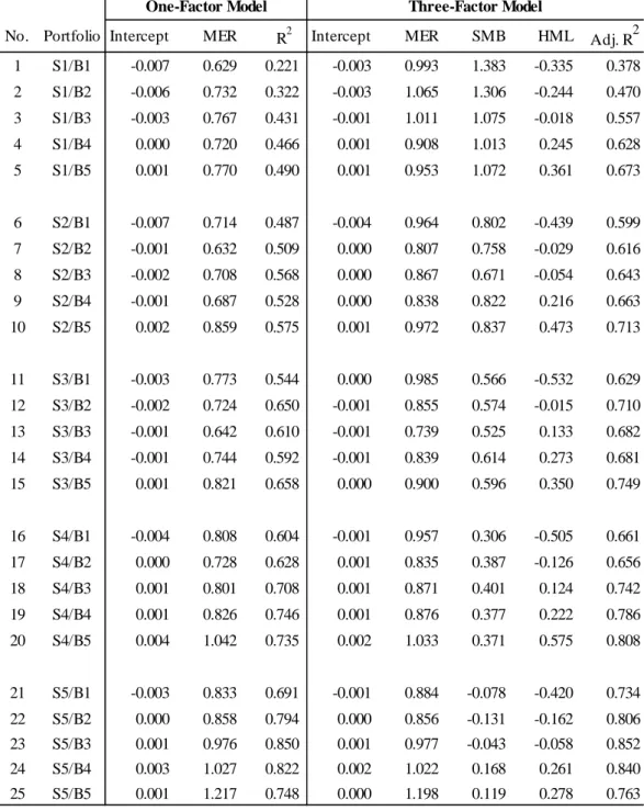
3.4 Cross-Sectional Analysis 10 Table 3 summarizes the results of time-series regressions for a one-factor model (with the market factor  ) and the three-factor model according to Eq. (1). The table shows coefficient estimates, -values for rejecting the null hypothesis of zero coefficients, and adjusted 2-values. The  quintiles are denoted by S1 to S5, the  quintiles by B1 to B5, both in ascending order.

Results for the one-factor model on the left-hand side of the table show that the factor   is important in explaining the time-series variations of stock returns. The coefficient estimates are close to one and statistically significant for all - portfolios. However, for some portfolios, the intercepts are significantly different from zero, which suggests that   alone does not fully explain the time-series variation of portfolio returns. The adjusted 2-coefficients are, on average, about 68%. In the three-factor model, coefficient estimates of   remain significantly positive for all 25 portfolios with values close to one. The most important result is that factor loadings on   decline from small to big  portfolios, and factor loadings on   increase from small to high  portfolios. 23 (of 25)   coefficients and 22 (of 25)   coefficients are significantly different from zero, so that both variables appear to capture factors driving stock returns. The adjusted 2_{-coefficients of the three-factor model are about}

80% on average, and none of the intercepts are significantly different from zero. Thus, results are in line with FF93.

– Insert Table 3 (p. 24) about here. –

3.4

Cross-Sectional Analysis

Another way to test the validity of the three-factor model is to examine whether the risk-related factors ( ,   and  ) explain the cross-section of stock returns. Firm characteristics other than risk factor sensitivities should not have explanatory power. To test this hypothesis, we proceed as follows. In the first step, we examine if cross-sectional differences between the raw returns of our 25 - portfolios can be explained by firm characteristics which have often been associated with return anomalies. In the second step, we repeat the analysis for risk-adjusted returns  which are defined as the part of raw returns not explained by the

3.4 Cross-Sectional Analysis 11 three-factor model:

= − ˆ1 − ˆ2 − ˆ3 

If the three-factor model fully captures the relevant return determinants, no systematic rela-tionship between characteristics and risk-adjusted stock returns will remain.

The characteristics we consider are , defined as a portfolio’s average market capitalization,  as the portfolio’s average  ratio, and three momentum variables16  2-3,  4-6, and  7-12 which capture the portfolio returns over the second through third, fourth through sixth, and seventh through twelfth month prior to the current month.17 _{We run monthly}

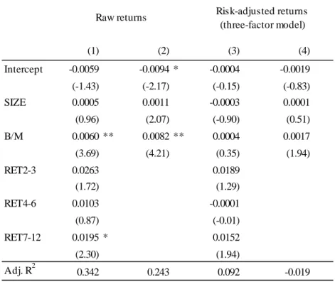
cross-sectional regressions for the 25 - portfolios according to the Fama and MacBeth (1973)-method. Table 4 shows the mean of the monthly slope coefficients and the corresponding -values (in brackets). For raw returns, the significantly positive coefficient of  indicates that a value premium is present at the European market during the sample period. The -coefficient is positive but insignificant. These findings confirm the evidence of Schrimpf et al. (2007), but are opposite to the results of Bauer et al. (2010) who do not find a value premium but confirm a premium for small stocks. In line with many studies on the momentum effect, the momentum coefficients are positive, with a statistically significant estimate for  7-12.18 On average, about one third of the cross-sectional variation of returns across the 25 portfolios in a given month is explained by portfolio differences in the firm characteristics (average adjusted 2 of 34.2%). Considering only the portfolio characteristics  and  leads to a smaller average adjusted 2 of 24.3%.

– Insert Table 4 (p. 25) about here. –

For risk-adjusted return () as dependent variable, the average adjusted 2 drops to 92%.

The remaining explanatory power only comes from the momentum variables. When these are

1 6

For the momentum anomaly, see, e.g., Jegadeesh and Titman (1993), Fama and French (1998), Rouwenhorst (1998) and Griffin et al. (2003).

1 7 _{We adopt the definition of the momentum variables  2-3,  4-6, and  7-12 from Brennan et al.}

(1998) and Bauer et al. (2010).

1 8

4 Empirical Effects of Portfolio Overlapping 12 excluded (last column), the 2 drops to zero. As  is no longer related to returns after the risk-adjustment, the three-factor model can be said to capture the value premium. Therefore, the value premium appears to be a risk premium compatible with rational asset pricing.

4

Empirical Effects of Portfolio Overlapping

The objective of this section is to examine whether the empirical results of the three-factor model are influenced by portfolio overlapping. We first present and employ a method based on random resampling (Section 4.1). Secondly, we exclude overlapping by splitting the sample into subgroups (Section 4.2). We then re-estimate the model to compare results with our earlier findings from Section 3.

4.1

Resampling Method (Randomization)

The idea of the resampling method is to break up any relationship between returns and variables  and  by randomly resampling stock returns. Specifically, the procedure consists of the following steps:

1. At the end of June of year  (sorting date), we collect the monthly stock returns of all firms  with  = 1      over the next 12 months. We denote the set of these stock returns by   = (1     12), where  is the stock return of stock  in the  -th month

after the sorting date .

2. For a given sorting date , we break up the firm-ordering of the  _· series and reassign them randomly to the firms (without replacement). This means that firm 1 is assigned the return series of a randomly chosen firm among the cross-section of  firms; firm 2 is then assigned the return series of a randomly chosen firm among the  − 1 firms not yet chosen, and so on. We denote the resampled return series assigned to firm  as  _∗  Due to the random reordering of returns across firms, the  _∗ returns will no longer be systematically related to  and .

3. In the same way as before, stocks are attributed to the (2x3)-building blocks of return factors   and   and the (5x5)-matrix of test portfolios. The portfolio composition

4.1 Resampling Method (Randomization) 13 is held constant for 12 months. The returns of these (2x3)- and (5x5)-portfolios for the 12 months after the sorting date are computed based on the resampled (randomized) return series. We denote the resulting return factors by  ∗ and  ∗ and the test portfolio returns by _∗

4. We run through steps 1. to 3. for all sorting dates (end of June each year) of the sample period.

5. We then run 25 time-series regressions of the test portfolio returns _∗ on  ∗  ∗ and the market proxy  . The outcome is a set of estimated regression coefficients. We repeat this resampling procedure (steps 1. to 5.) 500 times and compute the mean and standard deviation of the estimated regression coefficients. Note that the number of stocks in each of the (2x3)- and (5x5)-portfolios at any point in time is the same as before. Since  ∗ and  ∗ are return spreads based on randomly assigned stock returns, in an economic sense, they cannot account for any common variation of portfolio returns. Thus, significant regression coefficients are a reflection of portfolio overlaps.

There is an alternative way to interpret our resampling method. It is the same as a random reordering of pairs of (  ) within the cross-section of  firms at each sorting date ,

instead of a reassignment of returns. Let (∗_{ }∗₎

 denote the pair of  and  at

reordered rank . Then, ∗ and ∗ can be interpreted as new sorting variables. These new variables are designed such that they have the same cross-sectional distribution as  and  and are, by construction, not systematically related to stock returns. Based on the new sorting variables, the stocks are assigned to the (5x5)-test portfolios and the (2x3)-portfolios for computing  ∗and  ∗. Similar to the previous interpretation, factors based on randomly assigned variables should not be related to portfolio returns so that the average regression slopes would be zero without portfolio overlapping.

– Insert Table 5 (p. 26) about here. –

Table 5 reports the mean coefficient estimates over 500 runs of the resampled time-series regres-sions. The first three columns contain results for the one-factor model with the market excess

4.1 Resampling Method (Randomization) 14 return as sole explanatory variable, and the next columns contain results for the three-factor model. In the one-factor model, the average coefficient estimates are very similar across the 25 test portfolios. The structural differences disappear due to the random resampling of returns. The portfolio betas ( -coefficients) are close to 0.8 on average. The average beta is different from one, because the random resampling increases the importance of small stock returns (which can be resampled to small or large cap stocks). Since small stocks tend to have low betas in European stock markets, the average portfolio beta is below one. The intercept is significantly negative and almost the same for all test portfolios. This finding reflects the negative size effect on the European stock market during the sample period: the randomly resampled test portfolios underperform the market portfolio with its heavy concentration on large capitalization stocks. The underperformance is the same in the three-factor model. This is not surprising, because the added variables  ∗ and  ∗ are, by construction, unrelated to expected returns. The  -coefficients are again close to 0.8 for all test portfolios. Most importantly, the coefficients of  ∗ and  ∗both show a systematic pattern across test portfolios. Portfolios with small ∗_{-values have a significantly positive relation to  }∗ _{(portfolios 1 to 15 in Table 5), and}

vice versa for high ∗_{-portfolios (portfolios 16 to 25). Similarly, high }∗_-portfolios

(portfo-lios 5, 10, 15, 20, 25) are positively related to  ∗, while low-∗-portfolios (portfolios 1, 6, 11, 16, 21) obtain negative coefficients. The coefficients of  ∗ and  ∗ are clearly related to  and  of the test portfolios, although an economic relationship has been excluded by the randomization of returns. Almost all coefficients of  ∗ and  ∗ are statistically significant.19 The coefficients are particularly pronounced in the high ∗-group (portfolios 21 to 25). The overlap of these “∗-blue chips” with the ∗ part of  ∗ produces strongly negative coefficients with respect to  ∗. The adjusted 2-coefficient increases markedly compared to the one-factor model. In all, the apparent two-dimensional pattern due to the overlapping of portfolios confirms our hypothesis that the effect of overlapping is non-negligible. If it is not accounted for, results will be biased.

1 9

We compute conventional -statistics for the mean coefficients. The standard deviation of the mean corresponds to the sample standard deviation of coefficient estimates over the 500 resampling runs, divided by√500. Only the coefficients of  ∗ in the middle group of ∗ (portfolios 3, 8, 13, 18, 23) are not significant. All other -values for variables  ∗_{and  }∗_{are above 10}

4.2 Split Sample Results 15 Although our resampling approach shows the relevance of portfolio overlapping, it does not allow direct conclusions for the size of the bias in the estimated coefficients of our initial time-series regressions. The reason is that the - -test portfolios have specific return characteristics which are lost by randomization. In particular, the big cap portfolios with randomly assigned returns are no longer close to the market portfolio (with “real” returns). This is why the coeffi-cients of   of some “real” test portfolios strongly react to the inclusion of   and  , while they are insensitive to the inclusion of  ∗_{and  }∗ _{in the resampling approach (see}

the one-factor model compared to the three-factor model in Table 5). To obtain direct evidence on the quantitative impact of the overlapping problem on the estimated coefficients, the next section presents results based on the split sample approach proposed by FF93.

4.2

Split Sample Results

A simple way to exclude portfolio overlaps is to use different subsamples for determining the risk factors   and   on the one hand and the test portfolios on the other hand. We randomly divide our sample of firms in half. The first subgroup of firms serves to build each year’s (2x3)-portfolios for computing   and   The second subgroup is used to construct the (5x5)-matrix of test portfolios over time. Based on these variables, we run the 25 time series regressions in the same way as before. We repeat this procedure 500 times to make sure that the results are not specific to one particular random selection of subsamples.

– Insert Table 6 (p. 27) about here. – – Insert Table 7 (p. 28) about here. –

In Table 6, we report the average split sample coefficients, and in Table 7 the differences between the empirical coefficient estimates of Table 3 (based on the full undivided sample) and the average coefficients of the split sample approach. The general structure of the split sample results is similar to results of the standard approach, but the differences are nevertheless significant and systematic. As the split sample coefficients are not “contaminated” by portfolio overlaps, a positive difference can be interpreted as a positive bias of the standard empirical estimate, and

4.2 Split Sample Results 16 a negative difference indicates that the empirical estimate of the standard approach is too low due to the overlapping problem.

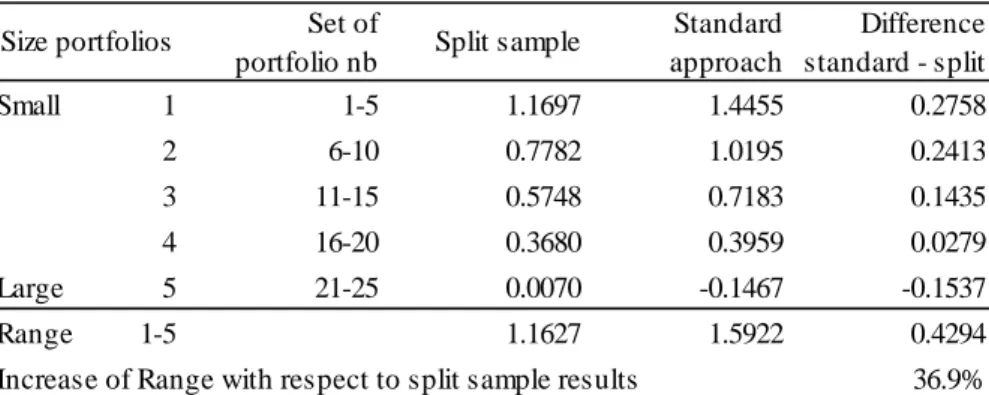
The differences for coefficients   and   in Table 7 are characterized by the same general patterns observed in the resampling section 4.1. To highlight these patterns, we show results in a more condensed form in Table 8. Panel A reports the mean  -coefficient for each of the five  groups, where the mean is computed across the five  -portfolios within the same  group. The respective portfolios included in the mean are indicated in column 3. The next columns show the coefficients of the split sample approach, the standard (full sample) approach, and the difference between these two. Panel B contains the same information for  -portfolios, where the means are taken across the five -portfolios within the same  group.

– Insert Table 8 (p. 29) about here. –

In the  dimension (Panel A), the differences are positive for small cap portfolios, negative for large cap portfolios, and decreasing in-between (see last column in Table 8). The standard approach produces a range of coefficients between the small and large size groups of 14455 − (−01467) = 15922 which is 36.9% larger than the respective range of the split sample approach. In the  dimension (Panel B), the coefficients for   are negative for low  -portfolios and positive for high  -portfolios. The negative  -coefficients of low  -portfolios as well as the positive  -coefficients of high  -portfolios are, on average, more extreme in the standard approach than in the split sample approach. The differences are statistically highly significant. Thus, the positive and negative associations of portfolio returns to   appear to be overly strong when the overlapping problem is present. Again, the differences seem important: the range of coefficients for low to high  -portfolios is −06834 − 05514 = −12348 in the standard approach, which is 44.7% higher than the same range of −08536 in the split sample estimation.

4.3 Cross-Sectional Analysis of Risk-Adjusted Returns 17

4.3

Cross-Sectional Analysis of Risk-Adjusted Returns

The previous chapters show that time-series coefficient estimates of the three-factor model (stan-dard approach) are biased due to the overlapping problem. Risk-adjusted returns will be different without the bias. Therefore, we recompute risk-adjusted returns based on the split sample ap-proach and rerun the cross-sectional regression of Section 3.4. The results are shown in Table 9.

– Insert Table 9 (p. 30) about here. –

For better comparison, columns two to five reprint the previous results of Table 4. Columns six and seven show the new coefficient estimates. The adjusted 2 and the  premium turn out to be higher than before. In contrast to the previous results, the  coefficient is even significantly positive if only  and  are included as explanatory variables. Thus, the ability of the three-factor model to capture cross-sectional return variation is lower when the overlapping bias is removed. Put differently, our results confirm the hypothesis that the standard approach of applying the three-factor model tends to overestimate the ability of the model to explain the cross-section of stock returns.

4.4

Relevance of the Number of Test Portfolios

As mentioned in the introduction, some studies use a smaller number of test portfolios. In this way, the test portfolios get closer to the (2x3)-building blocks of   and  , which is why the overlapping problem might become more important. As an attempt to assess the relevance of the number of test portfolios, we repeat all our analyses for a (4x4)- and (3x3)-matrix of test portfolios. We report the condensed results in Tables 10 and 11 which are structured in the same way as Table 8. The conclusions are basically the same as for the previous (5x5)-division. The differences between the split file results and the standard full sample estimation tend to be larger the smaller the number of test portfolios, but this effect is not dramatic.

References 18 – Insert Table 11 (p. 32) about here. –

5

Conclusion

Recent evidence on size- and value-related premiums at European stock markets is mixed. For example, Bauer et al. (2010) find a size effect but no value premium, while Schrimpf et al. (2007) identify a positive value premium but no size effect. Studying stock market anomalies based on unconditional models over the period from 1989 to 2009 for 16 European countries, we find evidence of significantly positive value und momentum premiums. The value premium is well captured by the three-factor model of FF93, while the momentum effect persists. These results are in line with prior evidence for the U.S. stock market.

In the time-series regressions of the Fama and French three-factor model, there is an overlap between test portfolios and factor mimicking portfolios, because both are formed on  and  . We use the empirical data from the first part of the paper to analyze the impact of portfolio overlapping in a realistic setting. We propose a resampling method and apply the split sample approach of FF93. The results clearly show that the overlapping is relevant and induces a non-negligible bias. The range of slope coefficients for - and  -portfolios is more than one third higher than in a setup without portfolio overlap. This means, that the standard approach overestimates the ability of the three-factor model to explain return variation and the cross-section of average returns. Specifically, it does not fully explain the value premium when an overlapping bias is absent.

The practical implication of this result is simple: the factor mimicking portfolios should be constructed from a different sample than the test portfolios. In small markets with a very small number of stocks, this rule might not be applicable. Thus, the coefficients of the standard time-series regressions will be biased and should be interpreted with caution. Rough corrections could be applied in robustness checks. However, small markets are typically not isolated. With a certain degree of international stock market integration, the relevant factors   and   are determined by international markets, so that the split file approach can be applied even if the test portfolios represent a single country.

References 19

References

Adrian, T. and Franzoni, F. (2009). Learning about beta: Time-varying factor loadings, expected returns, and the conditional CAPM, Journal of Empirical Finance 16(4): 537—556.

Amman, M. and Verhoven, M. (2008). Testing conditional asset pricing models using a Markov Chain Monte Carlo approach, European Financial Management 14(3): 391—418.

Ang, A. and Chen, J. (2007). CAPM over the long run: 1926-2001, Journal of Empirical Finance 14(1): 1—40.

Avramov, D. and Chordia, T. (2006). Asset pricing models and financial market anomalies, Review of Financial Studies 19(3): 1001—1040.

Bauer, R., Cosemans, M. and Schotman, P. C. (2010). Conditional asset pricing and stock market anomalies in Europe, European Financial Management 16(2): 165—190.

Berk, J. B. (2000). Sorting out sorts, The Journal of Finance 55(1): 407—427.

Brennan, M. J., Chorida, T. and Subrahmanyam, A. (1998). Alternative factor specifications, security characteristics, and the cross-section of expected stock returns, Journal of Financial Economics 49(3): 345—373.

Daniel, K. and Titman, S. (1997). Evidence on the characteristics of cross sectional variation in stock returns, The Journal of Finance 52(1): 1—33.

Daniel, K., Titman, S. and Wei, K. C. J. (2001). Explaining the cross-section of stock returns in japan: Factors or characteristics?, The Journal of Finance 55(2): 743—766.

Davis, J., Fama, E. F. and French, K. R. (2000). Characteristics, covariances and average returns: 1929 to 1997, The Journal of Finance 55(1): 389—406.

Dimson, E. and Marsh, P. (1999). Murphy’s law and market anomalies, The Journal of Portfolio Management 25(2): 53—69.

Faff, R. (2004). A simple test of the fama and french model using daily data: Australian evidence, Applied Financial Economics 14(2): 83—92.

Fama, E. F. and French, K. R. (1992). The cross-section of expected stock returns, Journal of Finance 47(2): 427—465.

References 20 Fama, E. F. and French, K. R. (1993). Common risks factors in the returns on stocks and bonds,

Journal of Financial Economics 33(1): 3—56.

Fama, E. F. and French, K. R. (1996). Multifactor explanations of asset pricing anomalies, Journal of Finance 51(1): 55—84.

Fama, E. F. and French, K. R. (1998). Value versus growth: The international evidence, The Journal of Finance 53(6): 1975—1999.

Fama, E. F. and French, K. R. (2012). Size, value, and momentum in international stock returns, Working paper.

Fama, E. F. and MacBeth, J. (1973). Risk, return and equilibrium: Empirical tests, Journal of Political Economy 81(3): 607—636.

Ferson, W. E. and Harvey, C. R. (1999). Conditioning variables and the cross section of stock returns, The Journal of Finance 54(4): 1325—1360.

Gibbons, M., Ross, S. and Shanken, J. (1989). A test of the efficiency of a given portfolio, Econometrica 57(5): 1121—1152.

Griffin, J. M. (2002). Are the fama and french factors global or country specific?, Review of Financial Studies 15(3): 783—803.

Griffin, J. M., Ji, X. and Martin, J. S. (2003). Momentum investing and business cycle risk: Evidence from pole to pole, The Journal of Finance 58(6): 2515—2547.

Guidi, M. and Davis, D. (2000). UK evidence on the 3-factor model and the glamour versus value controversy, Working paper.

Gustafson, K. and Miller, J. (1999). Where has the small-stock premium gone?, Journal of Investing 8(3): 45—53.

Heston, S. L., Rouwenhorst, K. G. and Wessels, R. E. (1999). The role of beta and size in the cross-section of european stock returns, European Financial Management 5(1): 9—27. Hodrick, R. and Zhang, X. (2001). Evaluating the specification errors of asset pricing models,

References 21 Jagannathan, R. and Wang, Z. (1996). The conditional CAPM and the cross-section of stock

returns, Journal of Finance 51(1): 3—53.

Jegadeesh, N. and Titman, S. (1993). Returns to buying winners and selling loosers: Implications for stock market efficiency, Journal of Finance 48(1): 65—91.

Lettau, M. and Ludvigson, S. C. (2001). Resurrecting the (C)CAPM: A cross-section of stock returns, Journal of Political Economy 109(6): 1238—1287.

Lewellen, J. and Nagel, S. (2006). The conditional CAPM does not explain asset pricing anom-alies, Journal of Financial Economics 82(2): 289—314.

Pastor, L. and Stambaugh, R. F. (2000). Comparing asset pricing models: An investment perspective, Journal of Financial Economics 56(3): 335—381.

Petkova, R. and Zhang, L. (2005). Is value riskier than growth?, Journal of Financial Economics 78(1): 187—202.

Rouwenhorst, G. K. (1998). International momentum strategies, The Journal of Finance 53(1): 267—284.

Santos, T. and Veronesi, P. (2006). Labor income and predictable stock returns, Review of Financial Studies 19(1): 1—44.

Schrimpf, A., Schroeder, M. and Stehle, R. (2007). Cross-sectional tests of conditional asset pricing models: Evidence from the German stock market, European Financial Management 13(5): 880—907.

Wang, K. Q. (2003). Asset pricing with conditioning information: A new test, Journal of Finance 58(1): 161—196.

Wu, X. (2002). A conditional multifactor analysis of return momentum, Journal of Banking and Finance 26(8): 1675—1696.

Zhang, L. (2005). The value premium, Journal of Finance 60(1): 67—103.

Ziegler, A., Schroeder, M., Schulz, A. and Stehle, R. (2007). Multifaktormodelle zur Erklärung Deutscher Aktienrenditen: Eine empirische Analyse, Schmalenbachs Zeitschrift für betrieb-swirtschaftliche Forschung 59(3): 355—389.

Figures and Tables 22

Table 1: Descriptive statistics of size and B/M portfolios

The table shows the average market capitalization, the average  ratio and the average number of firms for 25 portfolios in the period from July 1990 to December 2009. Portfolios are formed by sorting stocks independently on market capitalization () and book-to-market ratio ( ). Rows refer to  quintiles and columns to  quintiles, both in ascending order.

Low 2 3 4 High Small 612 599 626 592 604 2 1'464 1'477 1'489 1'488 1'503 3 2'507 2'501 2'498 2'539 2'561 4 4'906 5'196 5'087 5'089 5'012 Big 37'907 40'832 42'107 27'192 33'757 Small 0.25 0.37 0.55 0.73 1.16 2 0.18 0.36 0.50 0.68 1.10 3 0.19 0.35 0.48 0.66 1.06 4 0.16 0.34 0.48 0.67 1.03 Big 0.18 0.34 0.48 0.66 1.02 Small 29 30 28 32 45 2 34 34 29 33 34 3 34 31 36 31 32 4 33 32 34 34 31 Big 33 36 37 34 24

Book-to-market equity (B/M) quintiles

Average market cap (€ millions)

Average B/M ratio

Figures and Tables 23

Table 2: Average excess returns of size and B/M portfolios

The table presents average monthly excess returns of value weighted portfolios in the period from July 1990 to December 2009. Portfolios are formed by sorting stocks independently on market capitalization () and book-to-market ratio ( ). Rows refer to  quintiles and columns to  quintiles, both in ascending order. The portfolios are value weighted. H-L is the return differential between the high and low  portfolios; S-B is the return difference between the small and big size portfolios. The row and column denoted by “Mean” indicate the time-series mean of H-L (S-B) returns. The -values are based on a  -test of the hypothesis that H-L and S-B returns, respectively, are zero.

Low 2 3 4 High Mean H-L p-value (H-L) Small -0.0046 -0.0045 0.0003 0.0029 0.0042 0.0088 0.0078 2 -0.0039 0.0015 0.0014 0.0023 0.0051 0.0090 0.0005 3 -0.0004 0.0010 0.0018 0.0018 0.0046 0.0049 0.0472 4 -0.0004 0.0034 0.0031 0.0051 0.0081 0.0085 0.0014 Big 0.0004 0.0032 0.0045 0.0070 0.0060 0.0055 0.0354 Mean 0.0074 0.0000 S-B -0.0050 -0.0076 -0.0042 -0.0041 -0.0017 -0.0045 p-value (S-B) 0.1724 0.0206 0.1017 0.0724 0.5638 0.0007

Figures and Tables 24

Table 3: Time-series regressions for one-factor and three-factor model

The table shows the results of time-series regressions of the one-factor model = + _1 +  and the three factor model = + _1 + _2 + _3 +  The regressions are run for each of the 25 test portfolios sorted on  and  (monthly returns from July 1990 to December 2009). Portfolios are named as follows: ‘S’ refers to  portfolios and ‘B’ to  portfolios, ‘1’ denotes the smallest and ‘5’ the highest quintile. The columns include coefficient estimates, -values, and the adjusted 2. ‘#  0050’ denotes the number of -values smaller than 0.05. GRS F indicates the F-value of the Gibbons, Ross and Shanken (1989) test. The corresponding -value is shown in the line below.

No. Portfolio Interc. MER p-value (interc.)

p-value

(MER) R

2 _{Interc. MER SMB HML}p-value (interc.) p-value (MER) p-value (SMB) p-value (HML)Adj. R 2 1 S1/B1 -0.007 0.632 0.034 0.000 0.253 -0.002 1.123 1.765 -0.535 0.471 0.000 0.000 0.000 0.492 2 S1/B2 -0.007 0.725 0.014 0.000 0.359 -0.003 1.162 1.618 -0.415 0.228 0.000 0.000 0.001 0.572 3 S1/B3 -0.003 0.768 0.219 0.000 0.519 0.000 1.088 1.315 -0.119 0.874 0.000 0.000 0.204 0.702 4 S1/B4 0.000 0.730 0.967 0.000 0.535 0.000 0.962 1.250 0.328 0.825 0.000 0.000 0.000 0.778 5 S1/B5 0.001 0.760 0.609 0.000 0.547 0.001 0.984 1.279 0.413 0.421 0.000 0.000 0.000 0.803 6 S2/B1 -0.007 0.709 0.000 0.000 0.577 -0.002 1.076 1.102 -0.704 0.149 0.000 0.000 0.000 0.792 7 S2/B2 -0.001 0.635 0.469 0.000 0.618 0.001 0.889 0.991 -0.169 0.331 0.000 0.000 0.004 0.796 8 S2/B3 -0.002 0.730 0.303 0.000 0.674 0.001 0.967 0.909 -0.180 0.661 0.000 0.000 0.005 0.797 9 S2/B4 -0.001 0.681 0.750 0.000 0.621 0.000 0.881 1.058 0.252 0.960 0.000 0.000 0.000 0.848 10 S2/B5 0.002 0.859 0.437 0.000 0.643 0.000 0.998 1.037 0.599 0.749 0.000 0.000 0.000 0.851 11 S3/B1 -0.004 0.786 0.059 0.000 0.623 0.001 1.103 0.800 -0.819 0.388 0.000 0.000 0.000 0.777 12 S3/B2 -0.002 0.739 0.129 0.000 0.754 0.000 0.923 0.734 -0.098 0.687 0.000 0.000 0.071 0.842 13 S3/B3 -0.001 0.625 0.577 0.000 0.695 0.000 0.741 0.606 0.139 0.699 0.000 0.000 0.012 0.792 14 S3/B4 -0.001 0.738 0.424 0.000 0.679 -0.002 0.853 0.737 0.325 0.207 0.000 0.000 0.000 0.806 15 S3/B5 0.001 0.811 0.422 0.000 0.733 0.000 0.903 0.713 0.430 0.745 0.000 0.000 0.000 0.862 16 S4/B1 -0.004 0.799 0.024 0.000 0.703 0.000 0.996 0.355 -0.708 0.953 0.000 0.000 0.000 0.798 17 S4/B2 0.000 0.730 0.772 0.000 0.738 0.002 0.855 0.412 -0.186 0.161 0.000 0.000 0.005 0.767 18 S4/B3 0.000 0.801 0.889 0.000 0.780 0.000 0.883 0.475 0.156 0.892 0.000 0.000 0.011 0.824 19 S4/B4 0.002 0.808 0.152 0.000 0.812 0.001 0.855 0.399 0.266 0.291 0.000 0.000 0.000 0.860 20 S4/B5 0.004 1.047 0.020 0.000 0.804 0.001 0.999 0.338 0.764 0.480 0.000 0.000 0.000 0.902 21 S5/B1 -0.003 0.838 0.036 0.000 0.770 0.000 0.901 -0.188 -0.650 0.761 0.000 0.005 0.000 0.865 22 S5/B2 0.000 0.854 0.728 0.000 0.880 0.000 0.832 -0.268 -0.235 0.730 0.000 0.000 0.000 0.907 23 S5/B3 0.001 0.972 0.577 0.000 0.915 0.001 0.953 -0.130 -0.063 0.524 0.000 0.020 0.184 0.917 24 S5/B4 0.003 1.031 0.016 0.000 0.890 0.001 0.970 0.037 0.427 0.390 0.000 0.539 0.000 0.917 25 S5/B5 0.001 1.236 0.610 0.000 0.831 -0.002 1.104 -0.184 0.550 0.257 0.000 0.059 0.000 0.857 GRS F 0.615 # < 0.050 7 25 0.678 p-value 0.925 # < 0.050 0 25 23 22 0.805

Figures and Tables 25

Table 4: Cross-sectional regressions

The table reports average coefficient estimates and -values (in brackets) of monthly Fama/MacBeth regressions over the period from January 1991 through December 2009. Dependent variables are raw returns (columns 2 and 3) or risk-adjusted returns (columns 4 and 5) of 25 test portfolios sorted on  and  . Independent variables are the logarithm of a portfolio’s average market capitalization (), a portfolio’s average  ratio and three momentum variables ( 2-3,  4-6,  7-12). ∗ and ∗∗ denote significance at the 5% and 1% level, respectively.

(1) (2) (3) (4) Intercept -0.0059 -0.0094 * -0.0004 -0.0019 (-1.43) (-2.17) (-0.15) (-0.83) SIZE 0.0005 0.0011 -0.0003 0.0001 (0.96) (2.07) (-0.90) (0.51) B/M 0.0060 ** 0.0082 ** 0.0004 0.0017 (3.69) (4.21) (0.35) (1.94) RET2-3 0.0263 0.0189 (1.72) (1.29) RET4-6 0.0103 -0.0001 (0.87) (-0.01) RET7-12 0.0195 * 0.0152 (2.30) (1.94) Adj. R2 0.342 0.243 0.092 -0.019 Risk-adjusted returns (three-factor model) Raw returns

Figures and Tables 26

Table 5: Resampling method: Time-series regressions

The table shows the results of time-series regressions based on resampled returns. The regression equa-tions are ∗

 =  + 1 +  (one-factor model) and ∗ =  + 1 + 2 ∗+ _3 ∗

 +  (three-factor model), where superscript ∗ refers to resampled returns. The regressions are run for each of the 25 test portfolios sorted on  and  (monthly returns from July 1990 to December 2009). We repeat the resampling and the subsequent time-series regressions 500 times. Based on these 500 regressions for each test portfolio, the table reports the average coefficients and average ad-justed 2-values. Portfolios are named as follows: ‘S’ refers to  portfolios and ‘B’ to  portfolios, ‘1’ denotes the smallest and ‘5’ the highest quintile.

No. Portfolio Intercept MER R2 Intercept MER SMB* HML* Adj. R2

1 S1/B1 -0.001 0.801 0.715 -0.001 0.801 0.110 -0.132 0.719 2 S1/B2 -0.001 0.803 0.723 -0.001 0.802 0.131 -0.085 0.725 3 S1/B3 -0.001 0.802 0.708 -0.001 0.801 0.142 0.003 0.712 4 S1/B4 -0.001 0.804 0.730 -0.001 0.803 0.130 0.086 0.733 5 S1/B5 -0.001 0.802 0.768 -0.001 0.801 0.126 0.115 0.771 6 S2/B1 -0.001 0.806 0.755 -0.001 0.805 0.316 -0.330 0.768 7 S2/B2 -0.001 0.805 0.754 -0.001 0.804 0.321 -0.220 0.764 8 S2/B3 -0.001 0.806 0.733 -0.001 0.804 0.351 0.003 0.740 9 S2/B4 -0.001 0.805 0.754 -0.001 0.804 0.320 0.193 0.762 10 S2/B5 -0.001 0.806 0.761 -0.001 0.804 0.318 0.300 0.772 11 S3/B1 -0.001 0.804 0.757 -0.001 0.803 0.167 -0.234 0.764 12 S3/B2 -0.001 0.805 0.745 -0.001 0.804 0.168 -0.173 0.750 13 S3/B3 -0.001 0.804 0.765 -0.001 0.803 0.199 -0.010 0.768 14 S3/B4 -0.001 0.804 0.748 -0.001 0.804 0.126 0.151 0.752 15 S3/B5 -0.001 0.803 0.751 -0.001 0.802 0.170 0.263 0.759 16 S4/B1 -0.001 0.802 0.754 -0.001 0.801 -0.101 -0.109 0.757 17 S4/B2 -0.001 0.805 0.750 -0.001 0.804 -0.119 -0.090 0.752 18 S4/B3 -0.001 0.807 0.757 -0.001 0.807 -0.110 -0.001 0.759 19 S4/B4 -0.001 0.803 0.759 -0.001 0.802 -0.151 0.109 0.763 20 S4/B5 -0.001 0.802 0.740 -0.001 0.801 -0.156 0.178 0.744 21 S5/B1 -0.001 0.809 0.704 -0.001 0.807 -0.799 -0.821 0.767 22 S5/B2 -0.001 0.803 0.705 -0.001 0.801 -0.824 -0.528 0.748 23 S5/B3 -0.001 0.804 0.709 -0.001 0.803 -0.817 -0.019 0.737 24 S5/B4 -0.001 0.804 0.714 -0.001 0.803 -0.674 0.480 0.749 25 S5/B5 -0.001 0.805 0.633 -0.001 0.803 -0.911 0.926 0.712

Figures and Tables 27

Table 6: Split sample: Time-series regressions

The table shows the split sample results of time-series regressions of the one-factor model  = + _1 +  and the three factor model  = + _1 + _2 + _3 +  The factors   and   are built with one half of the sample, the test portfolios with the other half. The regressions are run for each of the 25 test portfolios sorted on  and  (monthly returns from July 1990 to December 2009). We repeat the random sample split and the subsequent time-series regressions 500 times. Based on these 500 regressions for each test portfolio, the table reports the average coefficients and average adjusted 2-values. Portfolios are named as follows: ‘S’ refers to  portfolios and ‘B’ to  portfolios, ‘1’ denotes the smallest and ‘5’ the highest quintile.Portfolios are named as follows: ‘S’ refers to  portfolios and ‘B’ to  portfolios, ‘1’ denotes the smallest and ‘5’ the highest quintile.

No. Portfolio Intercept MER R2 Intercept MER SMB HML _{Adj. R}2

1 S1/B1 -0.007 0.629 0.221 -0.003 0.993 1.383 -0.335 0.378 2 S1/B2 -0.006 0.732 0.322 -0.003 1.065 1.306 -0.244 0.470 3 S1/B3 -0.003 0.767 0.431 -0.001 1.011 1.075 -0.018 0.557 4 S1/B4 0.000 0.720 0.466 0.001 0.908 1.013 0.245 0.628 5 S1/B5 0.001 0.770 0.490 0.001 0.953 1.072 0.361 0.673 6 S2/B1 -0.007 0.714 0.487 -0.004 0.964 0.802 -0.439 0.599 7 S2/B2 -0.001 0.632 0.509 0.000 0.807 0.758 -0.029 0.616 8 S2/B3 -0.002 0.708 0.568 0.000 0.867 0.671 -0.054 0.643 9 S2/B4 -0.001 0.687 0.528 0.000 0.838 0.822 0.216 0.663 10 S2/B5 0.002 0.859 0.575 0.001 0.972 0.837 0.473 0.713 11 S3/B1 -0.003 0.773 0.544 0.000 0.985 0.566 -0.532 0.629 12 S3/B2 -0.002 0.724 0.650 -0.001 0.855 0.574 -0.015 0.710 13 S3/B3 -0.001 0.642 0.610 -0.001 0.739 0.525 0.133 0.682 14 S3/B4 -0.001 0.744 0.592 -0.001 0.839 0.614 0.273 0.681 15 S3/B5 0.001 0.821 0.658 0.000 0.900 0.596 0.350 0.749 16 S4/B1 -0.004 0.808 0.604 -0.001 0.957 0.306 -0.505 0.661 17 S4/B2 0.000 0.728 0.628 0.001 0.835 0.387 -0.126 0.656 18 S4/B3 0.001 0.801 0.708 0.001 0.871 0.401 0.124 0.742 19 S4/B4 0.001 0.826 0.746 0.001 0.876 0.377 0.222 0.786 20 S4/B5 0.004 1.042 0.735 0.002 1.033 0.371 0.575 0.808 21 S5/B1 -0.003 0.833 0.691 -0.001 0.884 -0.078 -0.420 0.734 22 S5/B2 0.000 0.858 0.794 0.000 0.856 -0.131 -0.162 0.806 23 S5/B3 0.001 0.976 0.850 0.001 0.977 -0.043 -0.058 0.852 24 S5/B4 0.003 1.027 0.822 0.002 1.022 0.168 0.261 0.840 25 S5/B5 0.001 1.217 0.748 0.000 1.198 0.119 0.278 0.763

Figures and Tables 28

Table 7: Split sample versus full sample results: Coefficient difference

The table shows the differences between the empirical coefficient estimates of a full sample (Table 3) and the average coefficent estimates of the split sample approach (Table 6).

No. Portfolio Intercept MER _R2 Intercept MER SMB HML _{Adj. R}2

1 S1/B1 0.000 0.003 0.032 0.001 0.130 0.382 -0.200 0.114 2 S1/B2 -0.001 -0.007 0.037 0.000 0.098 0.312 -0.171 0.102 3 S1/B3 0.000 0.002 0.088 0.001 0.078 0.241 -0.101 0.144 4 S1/B4 0.000 0.010 0.069 0.000 0.053 0.236 0.083 0.150 5 S1/B5 0.000 -0.010 0.056 0.000 0.032 0.207 0.052 0.130 6 S2/B1 0.000 -0.005 0.090 0.002 0.111 0.300 -0.265 0.193 7 S2/B2 0.000 0.003 0.108 0.001 0.082 0.233 -0.140 0.180 8 S2/B3 0.000 0.022 0.106 0.001 0.100 0.238 -0.126 0.154 9 S2/B4 0.000 -0.006 0.093 0.000 0.044 0.236 0.036 0.185 10 S2/B5 0.000 0.000 0.067 0.000 0.026 0.200 0.126 0.139 11 S3/B1 0.000 0.013 0.078 0.001 0.118 0.235 -0.288 0.149 12 S3/B2 0.000 0.016 0.104 0.001 0.068 0.161 -0.084 0.132 13 S3/B3 0.000 -0.017 0.085 0.000 0.001 0.081 0.006 0.109 14 S3/B4 0.000 -0.006 0.086 0.000 0.015 0.123 0.051 0.125 15 S3/B5 0.000 -0.010 0.074 0.000 0.004 0.117 0.080 0.114 16 S4/B1 0.000 -0.009 0.099 0.001 0.039 0.050 -0.203 0.137 17 S4/B2 0.000 0.003 0.110 0.000 0.020 0.026 -0.060 0.111 18 S4/B3 -0.001 -0.001 0.072 -0.001 0.012 0.074 0.032 0.082 19 S4/B4 0.000 -0.018 0.066 0.000 -0.020 0.022 0.045 0.074 20 S4/B5 0.000 0.005 0.069 -0.001 -0.034 -0.032 0.190 0.095 21 S5/B1 0.000 0.005 0.079 0.001 0.017 -0.110 -0.230 0.131 22 S5/B2 0.000 -0.004 0.086 0.000 -0.024 -0.137 -0.073 0.101 23 S5/B3 0.000 -0.004 0.065 0.000 -0.024 -0.087 -0.005 0.065 24 S5/B4 0.000 0.005 0.068 -0.001 -0.052 -0.131 0.165 0.077 25 S5/B5 0.000 0.019 0.083 -0.002 -0.094 -0.304 0.272 0.094

Figures and Tables 29

Table 8: Split sample versus full sample: Overview for (5x5)-test portfolios

The table compares the results of the full sample (standard) estimation (Table 3) and the split sample estimation (Table 6) in condensed form. Panel A reports the mean  -coefficients for each of the five  groups, where the mean is computed across the five  -portfolios within the same  group. Panel B contains the same information for  -portfolios, where the means are taken across the five -portfolios within the same  group. The column ‘Set of portfolio nb’ lists the portfolios included in the mean, where the portfolios are numbered as in Table 3.

Panel A:

Size dimension: mean coefficients with respect to SMB

Set of

portfolio nb Split sample

Standard approach Difference standard - split Small 1 1-5 1.1697 1.4455 0.2758 2 6-10 0.7782 1.0195 0.2413 3 11-15 0.5748 0.7183 0.1435 4 16-20 0.3680 0.3959 0.0279 Large 5 21-25 0.0070 -0.1467 -0.1537 Range 1-5 1.1627 1.5922 0.4294 36.9% Panel B:

B/M dimension: mean coefficients with respect to HML

Set of

portfolio nb Split sample

Standard approach Difference standard - split Low 1 1,6,11,16,21 -0.4462 -0.6834 -0.2372 2 2,7,12,17,22 -0.1152 -0.2207 -0.1055 3 3,8,13,18,23 0.0255 -0.0133 -0.0388 4 4,9,14,19,24 0.2435 0.3195 0.0760 High 5 5,10,15,20,25 0.4074 0.5514 0.1440 Range 1-5 -0.8536 -1.2348 -0.3811 44.7% Size portfolios B/M portfolios

Increase of Range with respect to split sample results

Figures and Tables 30

Table 9: Cross-sectional regressions based on split sample coefficients

The table compares the cross-sectional regression results of the split sample approach with the previous full sample (standard) estimation (see Table 4). For different model specifications, the table reports average coefficient estimates and -values (in brackets) of monthly Fama/MacBeth regressions over the period from January 1991 to December 2009. The regressions are based on 25 test portfolios sorted on  and  . Independent variables are the logarithm of a portfolio’s average market capitalization (), a portfolio’s average  ratio and three momentum variables ( 2-3,  4-6,  7-12). For ease of comparison, columns (1) to (4) are reproduced from Table 4. The risk-adjustment of portfolio returns (dependent variable) in columns (5) and (6) is based on the split sample estimation of the three-factor model. ∗ and ∗∗ denote significance at the 5% and 1% level, respectively.

(1) (2) (3) (4) (5) (6) Intercept -0.0059 -0.0094 * -0.0004 -0.0019 -0.0027 -0.0045 (-1.43) (-2.17) (-0.15) (-0.83) (-1.01) (-1.84) SIZE 0.0005 0.0011 -0.0003 0.0001 -0.0001 0.0004 (0.96) (2.07) (-0.90) (0.51) (-0.24) (1.50) B/M 0.0060 ** 0.0082 ** 0.0004 0.0017 0.0017 0.0032 ** (3.69) (4.21) (0.35) (1.94) (1.43) (3.36) RET2-3 0.0263 0.0189 0.0226 (1.72) (1.29) (1.52) RET4-6 0.0103 -0.0001 0.0032 (0.87) (-0.01) (0.28) RET7-12 0.0195 * 0.0152 0.0153 (2.30) (1.94) (1.93) Adj. R2 0.342 0.243 0.092 -0.019 0.117 0.005 Risk-adjusted returns (three-factor model) Risk-adjusted returns (three-factor model from

a split sample) Raw returns

Figures and Tables 31

Table 10: Split sample versus full sample: Overview for (4x4)-test portfolios

The table compares the results of the full sample (standard) estimation and the split sample estimation in the same way as Table 8, but only for 16 instead of 25 test portfolios (corresponding to a (4x4)-instead of (5x5)-sorting on  and  ). Panel A reports the mean  -coefficients for each of the four  groups, where the mean is computed across the four  -portfolios within the same  group. Panel B contains the same information for  -portfolios, where the means are taken across the four -portfolios within the same  group. The column ‘Set of portfolio nb’ lists the portfolios included in the mean, where the portfolio numbering follows the same rule as before.

Panel A:

Size dimension: mean coefficients with respect to SMB

Set of

portfolio nb Split sample

Standard approach Difference standard - split Small 1 1-4 1.1321 1.4171 0.2850 2 5-8 0.6319 0.8487 0.2169 3 9-12 0.4530 0.5120 0.0590 Large 4 13-16 0.0198 -0.1228 -0.1426 Range 1-4 1.1123 1.5399 0.4276 38.4% Panel B:

B/M dimension: mean coefficients with respect to HML

Set of

portfolio nb Split sample

Standard approach Difference standard - split Low 1 1,5,9,13 -0.3915 -0.6281 -0.2366 2 2,6,10,14 -0.0928 -0.1827 -0.0899 3 3,7,11,15 0.1874 0.2287 0.0413 High 4 4,8,12,16 0.3779 0.5240 0.1462 Range 1-4 -0.7694 -1.1521 -0.3827 49.7% Size portfolios B/M portfolios

Increase of Range with respect to split sample results

Figures and Tables 32

Table 11: Split sample versus full sample: Overview for (3x3)-test portfolios

The table compares the results of the full sample (standard) estimation and the split sample estimation in the same way as Tables 8 and 10, but only for 9 test portfolios (corresponding to a (3x3)-sorting on  and  ). Panel A reports the mean  -coefficients for each of the three  groups, where the mean is computed across the three  -portfolios within the same  group. Panel B contains the same information for  -portfolios, where the means are taken across the three -portfolios within the same  group. The column ‘Set of portfolio nb’ lists the portfolios included in the mean, where the portfolio numbering follows the same rule as before.

Panel A:

Size dimension: mean coefficients with respect to SMB

Set of

portfolio nb Split sample

Standard approach Difference standard - split Small 1 1-3 1.0073 1.2827 0.2754 2 4-6 0.5360 0.6676 0.1316 Large 3 7-9 0.0420 -0.0824 -0.1244 Range 1-3 0.9653 1.3651 0.3998 41.4% Panel B:

B/M dimension: mean coefficients with respect to HML

Set of

portfolio nb Split sample

Standard approach Difference standard - split Low 1 1,4,7 -0.3312 -0.5341 -0.2029 2 2,5,8 0.0265 0.0033 -0.0232 High 3 3,6,9 0.3449 0.4846 0.1398 Range 1-3 -0.6760 -1.0187 -0.3427 50.7% Increase of Range with respect to split sample results

Size portfolios

B/M portfolios

Figures and Tables 33

Figure 1: Cumulative factor returns

The figure below shows the cumulative returns of the factors MER, SMB and HML from July 1990 to December 2010. Date F a c to r re tu rn s 1990 1995 2000 2005 2010 -2 -1 0 1 2 3 _SMB HML MER

Authors

Martin WALLMEIER

Professor, Department of Finance and Accounting, University of Fribourg / Switzerland, Bd. de Pérolles 90, CH-1700 Fribourg, martin.wallmeier@unifr.ch

Kathrin TAUSCHER

Ph.D. candidate, Department of Finance and Accounting, University of Fribourg / Switzerland, Bd. de Pérolles 90, CH-1700 Fribourg, kathrin.tauscher@unifr.ch

Abstract

In the three-factor model of Fama and French (1993), portfolio returns are explained by the factors Small Minus Big (SMB) and High Minus Low (HML) which capture returns related to firm capitalization (size) and the book-to-market ratio (B/M). In the standard approach of the model, both the test portfolios and the factor portfolios SMB and HML are formed on the basis of size and B/M. This gives rise to a potential overlapping bias in the time-series regressions. Based on a resampling method and the split sample approach already proposed by Fama and French (1993), we provide an in-depth analysis of the effect of overlapping for a broad sample of European stocks. We find that the overlapping bias is non-negligible, contrary to what seems to be general opinion. As a consequence, the standard approach of applying the three-factor model tends to overestimate the ability of the model to explain the cross-section of stock returns.

Keywords

Asset pricing; three-factor model; portfolio overlapping; size effect; value premium

JEL Classification

G12, G14

Citation proposal

Wallmeier Martin, Tauscher Kathrin. 2012. «A Note on the Impact of Portfolio Overlapping in Tests of the Fama and French Three-Factor Model». Working Papers SES 433, Faculty of Economics and Social Sciences, University of Fribourg (Switzerland)

Working Papers SES

Last published :

426 Dafflon B.: Voluntary amalgamation of local governments: the Swiss debate in the European context; 2012

427 Wallmeier M.: Smile in Motion: An Intraday Analysis of Asymmetric Implied Volatility; 2012 428 Isakov D., Weisskopf J.-P.: Tre Founding Families Special Blockholders? An Investigation of

Controlling Shareholder Influence on Firm Performance; 2012 429 Gmür M.: Werden Frauen und Männer in NPO gleich bezahlt?; 2012

430 Reiser H., Gmür M.: Selbstverwaltete Betriebe zwischen Tradition und Markt; 2012

431 Bürgisser S.: Zusammenarbeit zwischen Vorstand und Geschäftsführung in Verbänden und andere Nonprofit Organisationen; 2012

432 Gmür M., Ribi Y.: Erfolgsfaktoren der Mitgliederbindung in Berufsverbänden; 2012

Catalogue and download links:

http://www.unifr.ch/ses/wp