Simulation based performance measures applied to new
technical analysis and portfolio optimization strategies
Thesis
presented to the Faculty of Economics and Social Sciences
at the University of Fribourg (Switzerland)
by
Didier MARTI
from Tschugg BE
in fulfilment of the requirements for the degree of
Doctor of Economics and Social Sciences
Accepted by the Faculty of Economics and Social Sciences on November 18
th, 2013
at the proposal of
Prof. Dr. Dušan Isakov (first advisor) and
Prof. Dr. Martin Wallmeier (second advisor)
ii
The Faculty of Economics and Social Sciences at the University of Fribourg neither approves nor disapproves the opinions expressed in a doctoral thesis. They are to be considered those of the author. (Decision of the Faculty Council of 23 January 1990)
iii
v
Preface
J'aimerais tout d'abord remercier mes parents qui m'ont soutenu et encouragé tout le long de mes études. En effet, mon début de parcours scolaire ne laissait pas penser à ce qu'il aboutisse à une thèse universitaire. Je tiens également à relever l'exemple fourni par mon grand frère, Claude-Oliver. En effet, je n'allais quand même pas le laisser être le seul Dr. Marti de la famille!
Ma seconde pensée va à mon directeur de thèse, le Prof. Dr. Dušan Isakov qui m'a guidé à partir de mon travail de Master et m'a activement introduit dans le monde de la recherche académique. Je lui suis particulièrement reconnaissant de sa confiance et de m'avoir laissé une grande liberté de recherche qui a rendu mes quelques années passées dans sa Chaire de Gestion Financière de l'Université de Fribourg très agréables et enrichissantes. J'aimerais également remercier le Prof. Dr. Martin Wallmeier pour son évaluation en tant que deuxième rapporteur.
Finalement, je remercie chaleureusement mes amis et anciens collègues de la faculté des sciences économiques. Je suis particulièrement redevable à Philippe Masset sans oublier Jean-Philippe Weisskopf, Florent Ledentu et David Ardia pour son expertise en économétrie.
A thinker sees his own actions as experiments and questions - as attempts to find out something. Success and failure are for him answers above all.
vii
Contents
Thesis introduction ... 19
Part I: A long term perspective on technical analysis strategies... 25
1. Introduction...25
2. Literature review...27
2.1 Complex trading systems ...28
2.2 Technical analysis profitability ...31
2.2.1 Studies in favour of technical analysis profitability ...31
2.2.2 Studies that find no technical analysis profitability...34
2.3 Evolution of profits across geographical areas and over time ...37
2.3.1 The market influence...37
2.3.2 Profit evolution through time...38
2.4 Why technical analysis may have forecasting power?...41
2.4.1 Market microstructure and uninformed traders...41
2.4.2 Nonlinearities in the price process ...42
2.5 A caveat about markets microstructure and data-snooping ...44
2.5.1 Microstructure issues...44
2.5.2 Data-snooping...45
3. The trading system...48
3.1 The simple MA rules ...48
3.2 The complex trading rules ...50
4. The investment strategies: Description and empirical results ...52
4.1 Statistical notations ...52
4.1.1 Returns characteristics ...52
4.1.2 Main performance measures...53
4.2 The standard investment setting...54
4.2.1 Data...55
4.2.2 The performance of the simple MA rule ...55
4.2.3 The complex trading system implemented in the standard investment setting ...58
4.2.4 The anatomy of the complex trading systems...62
4.3 Leverage with exchange-traded options ...64
viii
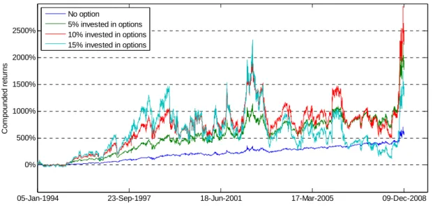
4.3.3 The performance of strategies using options ...70
4.4 Leverage with debt...75
4.4.1 Methodology and data ...75
4.4.2 Performance ...76
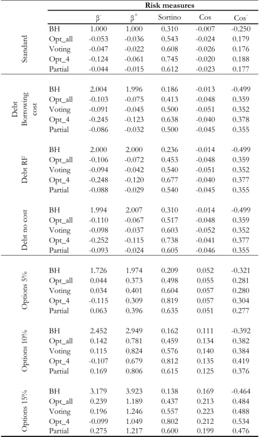
5. Other risk measures...79
6. A market timing test based on trading positions...83
6.1 Intuitions and methodology ...83
6.2 Results...85
7. Sign prediction and profitability ... 91
7.1 Intuitions and methodology ...91
7.2 Results...95
8. Conclusion...98
9. Appendices Part I ... 100
Part II: Portfolio optimization and parameter selection ...123
1. Introduction... 123
2. Literature review... 124
2.1 The empirical implementation of mean-variance optimization ...125
2.2 Enhancing the optimization ...127
2.2.1 The use of constraints ...127
2.2.2 The use of alternative parameters estimation methods: The means vector ...128
2.2.3 The use of alternative parameters estimation methods: The covariance matrix ...129
2.2.4 A comparison of alternative parameters estimation methods ...130
3. The investment strategy ... 133
3.1 The optimization process with various optimization specifications ...133
3.1.1 The optimization...133
3.1.2 The optimization inputs estimation...135
3.1.2.1 The assets means vector ...135
3.1.2.2 The assets covariance matrix...136
3.2 The construction of complex portfolios ...138
ix
5. Empirical results... 144
5.1 The optimization specifications ...144
5.2 Complex portfolios performance ...149
6. Conclusion... 156
7. Appendices part II... 157
Part III: A new simulation based market timing test...161
1. Introduction...161
2. Literature review... 164
2.1 Student t-tests ...164
2.2 Performance ratios...165
2.3 Tests based on asset pricing models...166
2.4 Market timing measures ...167
2.5 Simulation methods ...169
3. Student t-tests: a low-power testing procedure...171
4. The simulation test... 173
4.1 Introduction and intuition ...173
4.2 Single-asset case...173
4.3 Multiple-assets case...176
5. An application to technical analysis... 178
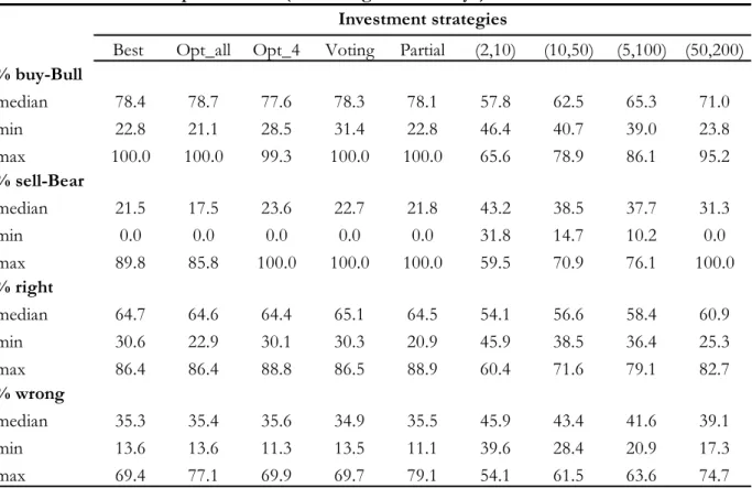
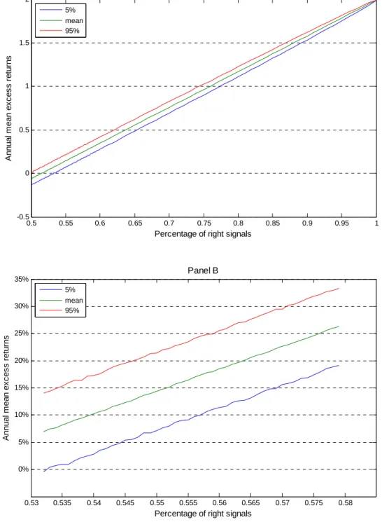
5.1 Percentage of right signals ...178
5.2 Complex trading rules in the standard investment setting...179
5.3 Complex trading rules with options ...184
5.4 Complex trading rules with debt...187
6. An application to mean-variance portfolios ... 189
7. A Monte-Carlo experiment... 193 7.1 Single-asset case...194 7.2 Multiple-assets case...205 8. Conclusion... 213 Thesis conclusion... 215 Bibliography ... 217
xi
List of tables
Table 1: Complex rules returns...59
Table 2: Out-of-sample performance of the Optim_4 strategy...64
Table 3: options returns descriptive statistics ...67
Table 4: Statistics of selected call and put options...69
Table 5: Options returns...71
Table 6: Complex rules returns with options...73
Table 7: Complex rules returns with debt leverage...77
Table 8: Other risk measures...82
Table 9: Rules positions during Bull and Bear markets...87
Table 10: Rules positions during Bull and Bear markets ...90
Table 11: Complex rules returns: Weekly frequency ...116
Table 12: Statistics of selected call and put options...120
Table 13: Strategies with option selected with a longer time to maturity...121
Table 14: Optimization specifications ...138
Table 15: Descriptive statistics with daily returns ...142
Table 16: Descriptive statistics with monthly returns ...143
Table 17: Estimation lengths versus parameters estimation models...147
Table 18: Difference in portfolios returns formed according to the estimation models ...148
Table 19: Portfolios performance analysis ...150
Table 20: Descriptive statistics...158
Table 21: Estimation lengths versus parameters estimation models...158
Table 22: Portfolios performance analysis ...160
Table 23: Percentage and right signals...179
xii
Table 26: Percentage and right signals – weekly frequency ...182
Table 27: Complex rules performance – weekly frequency...183
Table 28: Leverage with options...185
Table 29: Strategies with options...186
Table 30: Strategies with debt leverage...188
Table 31: Portfolios performance analysis ...190
Table 32: Simulation p-values and the length of the block bootstrap ...192
Table 33: Simulation p-values and the number of internal simulations ...193
Table 34: A comparison of tests power – 16 years...202
Table 35: A comparison of tests power – 8 years ...203
Table 36: Type I error for simulations tests...204
Table 37: Simulations and Student t-tests: Significant differences in returns ...208
Table 38: Simulation method and other performance measures – 16 years ...210
xiii
List of figures
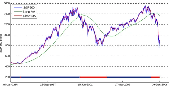
Figure 1: MA rule...49
Figure 2: Simple MA rules returns...55
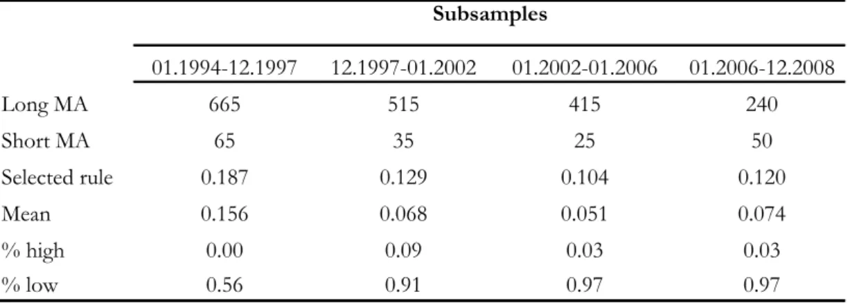
Figure 3: Simple MA rules returns on four subsamples...57
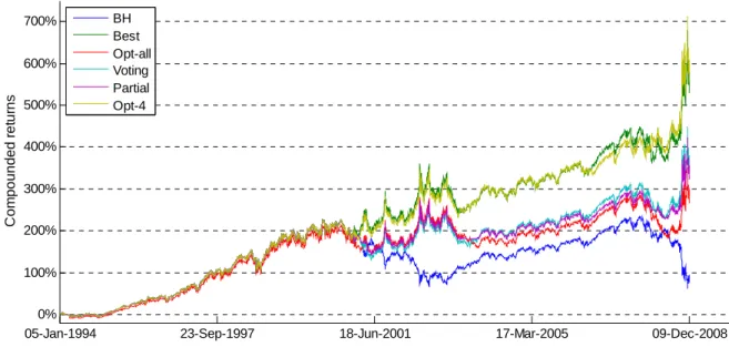
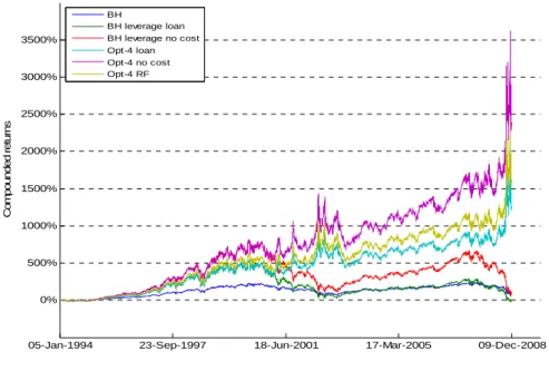
Figure 4: Complex rules compounded returns...61
Figure 5: Correlation between complex and simple trading rules ...63
Figure 6: Strike prices of options in our database...66
Figure 7: Opt_4 strategy compounded returns with options...74
Figure 8: Opt_4 strategy compound returns with debt leverage ...78
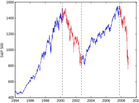
Figure 9: Bull and Bear markets...84
Figure 10: Opt_4 positions and the market phases ...89
Figure 11: Predictability and profitability: an illustration of the procedure...94
Figure 12: Percentage of right signals: a simulation...96
Figure 13: Hypothesis test ...101
Figure 14: Simple MA rules returns: Weekly frequency...115
Figure 15: Percentage of right signals: Weekly frequency...118
Figure 16: Estimation window lengths and parameters estimation models...145
Figure 17: Estimation window lengths selected ...149
Figure 18: Value of 1 USD calculated with compounded returns...153
Figure 19: Allocation in equity and the World index...154
Figure 20: Histogram of simulated Perf statistics...155
Figure 21: Estimation lengths versus parameters estimation models ...159
Figure 22: Student t-test power...172
Figure 23: Original and simulated trading signals ...176
xiv
Figure 26: Median p-values ...198
Figure 27: Some cross-sections...199
Figure 28: Percentage of significant tests ...200
Figure 29: Simulations and Student t-tests: median p-values ...207
xv
List of abbreviations
AR: Auto regressive
ARMA: Auto regressive moving average BH: Buy-and-hold strategy
BLL: Brock, Lakonishok and LeBaron (1992) CAPM: Capital Asset Pricing Model
CBOE: Chicago Board of Options Exchange DAX: Deutscher Aktien Index
DJIA: Dow Jones Industrial Average EMH: Efficient markets hypothesis
GARCH: Generalized Autoregressive Conditional Heteroskedasticity MA: Moving average
RC: Reality Check
RW: Random walk
S&P 500: Standard and Poor's 500 STA: Superior Predictive Ability TRB: trading range break-out USD: United States Dollar
xvi
1 A vector of ones
α: Strategy or portfolio alpha B: Bandwidth
β: Asset beta computed with respect to the market return Bl: Block length used in a block bootstrap simulation j: A portfolio optimization specification set
JB: Jarques-Bera statistic
Ku: Kurtosis
M: Markov chains transition probability matrix
Mt,S: Short moving average computed over the last S observations
Mt,L: Long moving average computed over the last L observations
Nb: Number of buy signals Ns: Number of sell signals N: Length of the time series
n: Number of assets in the portfolio optimization setting OA,t:: Option ask price at time t
OB,t:: Option bid price at time t
OC,t: Option closing price at time t
Pt: Index price
p: Markov chain state
Rt: Index return (equivalent to the buy-and-hold return)
R*
t: Simulated series return (a strategy or a artificial buy-and-hold series)
Rassets,t: Vector of assets returns used in the portfolio optimization setting
Ropt,t: Return of an option
RB,t: Borrowing rate
RC,t: Call option return
RDL,t: Return of a debt leveraged strategy
RL,t: Lending rate (or risk-free rate when only one rate is used)
RP,t: Put option return
RStrat,t: Return of an investment strategy (with or without leverage)
St: Trading signal at time t (1 for buy, -1 for sell and 0 for neutral)
S*
t: Simulated trading signal at time t (1 for buy, -1 for sell and 0 for neutral)
SBH,t: Dummy variable that takes a 1 (-1) if the market is in a bull (bear) phase
xvii
St*: A statistic computed with a simulated strategy returns series
Sk: Skewness
SBt:: One if the strategy generates a buy signal at time t, zero otherwise
SSt: One if the strategy generates a sell signal at time t, zero otherwise
σ: Standard deviation
Σt: Covariance matrix used as input in the portfolio optimization ΣSt: Sample covariance matrix
TC: One-way transaction cost
UPt: Option underlying price at time t
μt: Expected returns vector used as input in the portfolio optimization
X: Option strike price
xt: Mean-variance optimal portfolio weights
W*
t: Simulated portfolio weights
Thesis introduction
The efficient market hypothesis (EMH) is a pillar of the modern finance theory. It asserts that financial markets integrate all information immediately and accurately. Fama (1970) further define the EMH by proposing three levels of efficiency; the weak, semi-strong and strong form. They differ according to the kind of information considered; the first case states that past prices contains no useful information to predict future prices movements, the second supposes that prices are adapted immediately to all publicly known information, while the last form suggests that all information, including the private and hidden one, is reflected in prices. The EMH implies that prices follow a random walk, and thus, are not predictable. Jensen (1978) further differentiates between the statistical predictability and the economic performance. He argues that a market is efficient with respect to a set of information if it is not possible to generate economic profits, once the returns are adjusted to risk and transaction costs are taken into account. Thus, an investor should expect a normal return on his portfolio, which is defined according to the amount of risk that he accepts to bear.
Despite the importance of this hypothesis in the academic literature, the financial industry is based on the opposite idea; active management is able to outperform its benchmark, either by timing the market or by selecting investment opportunities that are not correctly priced by the market. This is illustrated by the large amount of actively managed funds proposed to investors and the amount of predictions about the market evolution and companies future earnings and returns found in the financial media. A major motivation for the academic literature about active asset management is that investment methods that have been either introduced or improved by academic studies are widely used in practise. For instance, several surveys indicate that professional money managers commonly employ technical analysis methods. In addition, Amenc, Goltz and Lioui (2011) show that standard or a variation of the mean variance optimization, introduced by Markowitz (1952), to construct portfolios is also widely used by asset managers in Europe. As a concrete example, we may cite the various funds belonging to the "QUAM" family
proposed by the asset manager "Edmond de Rothschild PriFund"1. They consist in a purely
mathematical approach to construct their portfolio, which is largely inspired by the standard mean variance optimization method.
As a consequence, a myriad of studies examine whether assets returns are predicable, whether mutual funds investing is more valuable than a buy-and-hold strategy and whether investment strategies based on past information, such as technical analysis, momentum or value/growth strategies, are profitable. These studies are a mean to test the EMH, and while we do not pretend to provide a comprehensive literature review about these issues, we present some of the major studies briefly.
First, Keim and Stambaugh (1986), Ferson and Harvey (1993), or more recently Ang and Bekaert (2007) find that stocks or bond returns can be predicted, at least to some extent, with lagged variables such as the credit-risk spread, the term structure of interest rates or the dividend yield. Cochrane (2008) argues that as the dividend growth is not predictable, then returns should be predictable in order to have the observed variation in the dividend yield. In addition, Lo and MacKinlay (1988) find that stock returns do not follow a random walk, but they also point out that this result is not a sufficient proof to reject the EMH. Second, in addition to these studies supporting some level of predictability, many investment strategies, which can be either explicit or result from anomalies in stock returns, appear to be able to generate abnormal returns. For example, Brock, Lakonishok and LeBaron (1992) show that simple technical analysis strategies are able to outperform the buy-and-hold performance. Jegadeesh (1990), Jegadeesh and Titman (1993) and Lakonishok, Shleifer and Vishny (1994) document various aspects of prices reversal or momentum according to the temporal horizon. Among the anomalies that are used to develop investment strategies, we may cite the size and the calendar effects and the highest return obtained by value stocks compared with growth stocks.
Nonetheless, despite all these elements, the literature on the performance of actively managed mutual funds inclines toward the validity of the EMH. Indeed, most of these studies find that the vast majority of funds are not able to provide a higher risk-adjusted performance than passively investing in the benchmark. This raises the question about the opportunity to exploit the returns predictability and these anomalies in a real trading setting. Indeed, transaction costs, the
1 A prospectus can be freely downloaded on the "Banque Privé Edmond de Rothschild" website. No direct link is provided as each user has to be identified first.
1. Introduction 21 mining issue, an incomplete risk adjustment are among the reasons why these findings may only hold in academic studies. Malkiel (2003) presents a review of these anomalies. While he does not pretend that market prices are always perfectly set, he questions the presence of trading opportunities that would enable to earn a risk-adjusted abnormal return. However, the jury is still out on whether this hypothesis is valid or not.
As empirical studies about investment strategies require a testing procedure in order to determine whether a risk adjusted abnormal return can be obtained, we consider these two issues with a common framework. In a first step, we focus on investment strategies that mainly use equity indices as their investment universe. We analyse some new specifications of well-known investment strategies, i.e. technical analysis and mean variance portfolio optimization. We choose them as they are widely used in practice and they do not involve any subjectivity from the manager in their construction. The second objective is to point out the importance of the testing procedure used to determine if a strategy generates abnormal returns, and to propose a new technique based on the simulation of trading positions. Indeed, the performance measure is primordial both for professional managers and for academics. The former's remuneration and overall success depends on it and for the latter, it may provide evidence in favour or against the EMH.
The overall structure of this thesis is the following: In the first Part, we examine in detail some new technical analysis strategies based on moving-averages. The novelty of our approach resides in exploiting long-term trends, as we use long moving-averages up to four years, while other studies only consider trends up to one year. Indeed and to the best of our knowledge, we are the first to examine commonly used technical trading rules in a long-term setting. As data-snooping is always an issue of this kind of study, we focus on out-of-sample processes that select the parameters used by the investment strategy objectively. We find that our rules produce returns twice as high as the benchmark over a 15 years sample. Then, we propose a new market timing test that focuses on market phases, i.e. bull and bear markets, and we show evidence supporting the fact that the trading strategy invests according to these trends. Consequently, it changes trading position very rarely, and thus, common issues such as transaction cost or market microstructure do not impact its effective implementation. Nonetheless, despite its strong economic performance, Student t-tests are not able to reject the null hypothesis of equal means, between the strategy and the benchmark.
The second Part is dedicated to mean-variance optimal portfolios. Specifically, we investigate the impact of using various lengths of the estimation window. Indeed, this aspect is seldom addressed in the related literature, which usually focuses on developing sophisticated parameters
estimation models. First, we show that using shorter lengths than the standard five years for the estimation window improves the optimization performance dramatically. Moreover, this aspect of the inputs estimation seems to affect the performance to a greater extent than the choice of various popular estimation models. However, as the optimization specification2 has to be chosen
arbitrarily, the data-snooping issue arises again. Hence, we propose to employ selection processes that are similar to the ones used in the technical analysis setting. We show that the resulting portfolios generate large excess returns compared with the equally weighted portfolio. However, the performance strongly depends on the ability to take short positions and the level of transaction costs. In contrast with the results obtained for the technical analysis strategies, the optimal portfolios, despite their large returns, can probably not challenge the EMH.
Finally, the last Part re-examines the conclusions of the first, i.e. the technical analysis strategies can produce large abnormal returns that are not statistically significant. We argue that the standard Student t-test used to determine statistically whether a strategy mean return differs from its benchmark is not a powerful procedure. Indeed, we first show that a strategy should generate a return at least three times as high as the benchmark strategy in order to find a statistically significant difference. Hence, we propose a new test based on the simulation of trading positions. This approach is not new; however, our proposed test is designed to keep the structure of the original trading positions. As the strategy invests according to long-term trends and changes trading positions very rarely, we argue that the artificial positions series should have a similar pattern. We propose to model the trading positions as first-order Markov chains. This has the merit to limit the number of assumptions to only one; the next trading signal depends on the current one only. Thus, we do the performance analysis, presented in the first part, once again with the proposed test, and we find that all p-values associated with various performance measures are lower than the standard 5% confidence level. This means that the large abnormal returns can not be replicated by taking random positions, with a similar structure to the original one, in the market. The difference in conclusions between the two testing procedure in striking: With Student t-tests, we would conclude that the strategies possess some predictive power, but it can not generate statistically significant abnormal returns. This contrasts sharply with our proposed simulation test that concludes that the performance is neither due to luck nor to risk bearing.
2 By specification, we mean the models used to estimate the parameters and the window length over which the estimation is performed.
1. Introduction 23 We also adapt the simulation test to strategies that invest in more than one asset simultaneously, such as the optimal portfolios examined in the second Part. In this case, the Markov chains are not suitable, thus, we propose to use a block bootstrap to keep the dependencies in the portfolio weights at least to some extent. Then, we apply this test to these portfolios and compare the results with standard Student t-test. The findings are in line with those related to technical analysis, even if the difference in conclusions with a 5% confidence level is less marked.
To conclude this last Part, we conduct a comprehensive Monte-Carlo experiment to compare the power of various testing procedures. We focus on the level of abnormal returns required to reject the null hypothesis of equal performance. We find that the proposed simulation test power is more than or at least equal to Student t-tests computed on several performance measures, such as the difference in mean returns, the Sharpe ratio or the Jensen’s alpha. Nonetheless, large economical returns are necessary to reject the null, even with our test.
Part I: A long term perspective on technical analysis
strategies
1. Introduction
Technical analysis comprises a wide range of methods used to forecast future price movements of stocks, currencies or commodities, based on their past prices and volumes. These methods may be classified into two broad categories, charting and technical trading systems. The first group consists of methods analysing charts to detect price patterns that are supposed to repeat themselves. The second group includes a variety of quantitative rules aimed at detecting trends and generating trading signals accordingly. Among them, the moving average, referred to as MA thereafter, and the filter trading rule are the most popular3.
Several surveys conducted with professional investment mangers show that the vast majority of them use technical analysis to some extent. Allen and Taylor (1990) in the London foreign exchange market, Lui and Mole (1998) in Hong Kong and Oberlechner (2001) in various European markets document that technical trading is broadly used in order to forecast short-term trends. These surveys also point out that its utilization by professional diminishes as the forecasting horizon increases. In addition, these techniques are not regarded as being in contradiction with fundamental analysis, but they are used in a complementary approach. According to Gehrig and Menkhoff (2006), the use of technical analysis increases during the
3 In this thesis, the trading rule relates to the method according to which trading signals are generated. The trading system
consists in using more than one indicator to produce these signals. Strategies reflect the effective positions taken in the market by either combining long and short position or using financial leverage.
nineties. They reach this conclusion by comparing surveys conducted in 1992 and again in 2001 among German and Austrian foreign exchange dealers and funds managers.
On the other hand, academics have been skeptical about the utility of these forecasting methods. Among the various conceivable reasons, we can mention that they lack a sound theoretical basis and the parameters selection is usually not disclosed or justified. In addition, empirical evidence of technical trading profitability is mixed, and strongly depends on the choice of the time interval, the set of methods considered or the underlying asset. Another concern about technical analysis arises as reported evidence of profitability may be biased by data-snooping issues. Indeed, using the same data and trading rules repeatedly may lead to find a few profitable rules by luck.
The objective of this first Part is to examine some new MA strategies based on the out-of-sample approach of Sullivan, Timmermann and White (1999), Skouras (2001) and Fong and Yong (2005). Instead of choosing the parameters arbitrarily, we utilize various selection processes that combine or select trading signals issued by simple MA rules. Furthermore, we extend the literature by considering a much wider range of parameters, for both the short and the long MA. Indeed, all studies related to MA trading rules focus on short-term trends, as they use a long MA up to only 200 or 250 days usually. To the best of our knowledge, nobody examines MA rules in a long-term setting, with parameters longer than 250 days. Indeed, long-term trends may be more easily identified, and they may be less noisy than their short-term counterparts. In addition, there is a possibility that when a short-term trend is identified, it is already too late to exploit it. We find evidence that our trading systems provide much higher returns than usual MA rules. The annual mean returns of our strategies lie between 10.7% and 14.6%, compared with 6.1% for the buy-and-hold. Moreover, the strategies are especially profitable during the most recent period, while the majority of studies find that the technical analysis performance decreases over time. However, Student t-tests fail to reject the null hypothesis of equal means between the strategies and the benchmark. Appendix I-A presents a statistical reminder about these tests. In Part III, we argue that these results are due to the Student t-test low power, and thus, we propose a more powerful test based on the simulation of trading signals. In this first part, we also develop a new market timing test that determines whether a strategy relies on long-term trends related to the business cycle. We find that the strategies trading position coincide with bull and bear market phases to an extent that can not be achieved by luck.
A second objective of this first Part is to examine technical strategies with financial leverage. Indeed, technical trading is widely used by commodity trading advisors (CTA), a class of hedge funds, which may rely on financial leverage to increase the performance. For this purpose, we
2. Literature review 27 consider debt leverage and exchange-traded options. However, we first ensure that the complex rules possess significant forecasting abilities. Indeed, using leverage without these abilities should not add any significant value after the risk adjustment. A second reason for using financial leverage lies in the possibility that even successful forecasting methods may not generate abnormal returns if the market follows a strong upward trend. We find that the superior performance of debt leveraged strategies could not be attributed to leverage itself, but to their predictability. This contrasts with options based strategies, which are not profitable mainly because of the loss of time value. Finally, we provide some insights about the strategies performance analysed with alternative risk measures, which include higher moments of the returns distribution. We show that our strategies are attractive as they may hedge skewness risk without sacrificing returns.
Finally, we perform a simulation analysis to shed light on a puzzling aspect of our results. Indeed, we find that strategies yield economically significant returns in excess of the buy-and-hold. However, we also find that their percentages of correctly predicted trading signals are only slightly higher than the buy-and-hold. Thus, we examine this relationship, and we conclude that only a small increase in these percentages leads to high excess returns.
The structure of this Part is the following: Section 2 presents a comprehensive literature review about related studies. In Section 3, we describe the trading systems. Section 4 includes the description and the empirical implementation of the trading strategies. It is divided in four parts; the first one examines the performance of the simple MA rules to shed light on the impact of using an extended set of parameters, while the three other ones display the performance analysis of the strategies without leverage, with options or with debt. Section 5 displays a risk analysis with alternative measures. In Section 6, we describe and implement our new market timing test based on market phases. In Section 7, we conduct a simulation experiment to explain the relationship between the percentage of right signals and a strategy performance in excess of the buy-and-hold. Finally, Section 8 concludes.
2. Literature review
In this literature review, we provide a rather comprehensive overview that do not only covers the issues investigated in this thesis, but also other important aspects that decide whether abnormal returns can be obtained in a real trading setting. Specifically, it focuses on the various proposed trading systems, which combine several simple technical indicators. Appendix I-B
briefly presents the most commonly used simple trading rules. Then, we summarize studies related to the performance of technical analysis, and the underlying reasons why technical analysis may be useful as a prediction method. This review focuses on papers that apply trading rules to equity indices or stocks, but we sometimes refer to studies on foreign exchange when they provide some interesting methodological aspects.
2.1
Complex trading systems
Here, we define a complex trading system, or complex trading rules, as a procedure that combines several simple technical trading indicators to generate trading signals. The objective is to use more information than a single indicator, but also to take into account various aspects considered by the simple indicators. Some others trading systems, referred to as complex rules, are based on a selection and an out-of-sample test sample. These methods should mitigate the data-snooping bias.
The most straightforward way to combine several trading signals is simply to compute them independently, and then, take a position only if they reach a consensus. Pruitt and White (1988) propose the CRISMA trading system, which stands for “Cumulative volume, Relative strength, Moving Average” and combines three simple technical indicators. The system takes a position only if the three indicators generate the same signal. Fang and Xu (2003) follow the same method to compute complex trading signals. They combine MA rules signals with time series forecasts generated by different models, such as the auto-regressive model or various kinds of GARCH models. They show that these two forecasting methods capture different aspects of the price predictability, and thus, are complementary. Indeed, the MA rules tend to produce better forecasts for upward trends, while time series forecasts are more accurate for detecting downward trends.
Gençay, Dacorogna, Olsen and Pictet (2003) examine the performance of a commercial real-time trading model, the RTT model, developed by Olsen & Associates. It uses a trend following technique based on an equally-weighted iterative moving average of 20 days. In addition, it also determines the percentage of the capital to be invested according to the strength of the trading signal. This contrasts with most of the technical analysis strategies that either invest the entire capital or take a short position corresponding to the whole capital. The trading system also contains a contrarian indicator to diminish the position exposure to extreme exchange rate movements. Nevertheless, such a position against the current trend may be taken only if the profitability has already reached a yearly return objective level, set at 3%. The authors argue that
2. Literature review 29 analysing this model may shed light on the usefulness of technical analysis, as its performance may proxy very well those of an investor (or a currency dealer) in a real trading setting. Indeed, it considers intraday data, transaction costs with the bid-ask spread, real trading hours and the model trading frequency is in line with those of a real trader.
Bessembinder and Chan (1998) use a portfolio approach to aggregate the set of 26 rules used by Brock, Lakonishok and LeBaron (1992), referred as to BLL thereafter. They allocate an equal fraction of the invested capital according to the signal emitted by each rule. This is also a way to avoid, or at least to minimize, the data-snooping bias resulting from using only the best rules in an in-sample analysis. A slightly different approach is proposed by Chang and Osler (1999). Their strategy takes a position twice as large as usual if both the head-and-shoulders signal and a signal issued by the most profitable MA or momentum rule coincide. Otherwise, the system does not take any position.
Another way to combine signals from simple technical indicators is to use selection algorithms. They consist in selecting, during an evaluation interval, some rules specifications according to a criterion. Then, these specifications are evaluated over an out-of-sample test interval. Hsu and Kuan (2005) implement complex trading rules4 only based on simple technical
indicators, such as MA rules, trading range break-out (referred as to TRB thereafter) and head-and-shoulders among others. They implement three kinds of strategies in order to combine the signals issued by the simple rules. The first is a learning strategy that selects the best-performing specification from a particular class of rules during a predetermined test sample. The second is the voting strategy that gives one “voting right” to each specification, and the system uses the position that has received the largest number of votes. The last one, the fractional position strategy represents an average of the signals produced by all specifications inside a class of rules5.
The purpose of these complex strategies is to reach a consensus by using more information than it would be possible with a single indicator. Skouras (2001) proposes to use only MA rules with a short window restricted to one day. Nevertheless the length of the long window is not constrained to take a predetermined value, such as 10, 20, 50, 100 or 200 days, which is usually done in other studies. Here, he considers all values from one to 200 days. He shows that the
4 The rules considered by our empirical work are closely related to them. Thus, more details are given thereafter.
5 For instance, if the 55 MA rules generate 32 buy and 23 sell signals, the position taken by the complex strategy is a long
optimal rule chosen by the so called “artificial technical analyst” varies significantly through time and presents pronounced discontinuities. Fong and Yong (2005) consider a similar approach but without restraining the short MA to one day. Lee and Mathur (1996), Maillet and Michel (2000) and Olson (2004) employ an easier procedure: They divide their sample in five years subsamples and apply the best in-sample rule to the next out-of-sample period. Moreover, these strategies are a way to conduct out-of-sample tests, as the parameters are not, or to a lesser extent, chosen arbitrarily at the beginning of the sample. Furthermore, by comparing the performance of a complex strategy with the best rule over the whole sample, we can determine whether the trading system is able to identify the best rule ex-ante. For instance, Cooper (1999) shows that out-of-sample profits are between 25% and 40% lower than those obtained during the in-out-of-sample interval used to select the parameters.
Finally, some methods inspired by biology models are adapted to generate trading programs. Allen and Karjalainen (1999) propose a genetic program to combine simple MA and trading range break-out rules to produce “optimal” complex trading rules. They are generated during an estimation and validation period, and then, they are applied to an out-of-sample test period. The idea is to combine simple rules by weighting them according to a fitness criterion, in this case the return of the rule in excess the buy-and-hold. While it is appealing in the sense of minimizing the in-sample selection bias, these complex systems may have a very complex structure, and thus, they are rather difficult to interpret. Neely, Weller and Dittmar (1997) use a similar method with another criterion, as they apply the genetic program to foreign exchange markets. Thus, they do not use the return of the strategies in excess of the buy-and-hold, but they adapt the returns to the interest rate differential. This approach to generate trading rules is also examined by Neely (2003) with an emphasis on risk, Potvin, Soriano and Vallée (2004) with individual Canadian stocks and Neely and Weller (2003) with intraday data. Finally, Brabazon and O’Neill (2004) propose a grammatical evolution model inspired by the biological process of mapping of genes to proteins6. They use MA, momentum and TRB indicators as inputs into their evolutionary
automatic programming model to generate complex trading rules. They also consider the maximal drawdown as the fitness criterion to account for risk and to avoid extreme losses.
2. Literature review 31
2.2 Technical analysis profitability
This review focuses on modern studies on the stock market, starting with Brock, Lakonishok and LeBaron (1992). Indeed, they usually include several risk measures and a comprehensive performance analysis. For a comprehensive review of early studies, the interested reader may refer to Park and Irwin (2007).
2.2.1 Studies in favour of technical analysis profitability
Brock, Lakonishok and LeBaron (1992) find that simple technical trading rules (MA and TRB) applied to the DJIA over a century of data produce significant excess returns. In addition, they implement a bootstrap technique to address some limitations of traditional hypothesis tests with Student t-tests, such as the hypothesis of normal returns. They find that the profitability can not be replicated by rules simulated on prices series obtained with various returns generating models, such as the random walk or GARCH models. Their methodology, i.e. the set of rules and the bootstrap test, has influenced a multitude of studies using the same approach for various time intervals and markets. Skouras (2001) shows that using a selection method to find the “optimal” MA rule parameters results in both higher returns and their associated t-statistics. The latter test whether returns are different from the buy-and-hold or zero, and they are much higher than those obtained, on average, by BLL. The difference is also economically significant, as the profits generated by the optimal rule are more than three times higher than those obtained by BLL. Fong and Ho (2001) find that basic trading rules based on MA are profitable when they are tested on US Internet stocks, even after considering transaction costs and a time-varying risk premium. Moreover, they argue that these profits result from the rules predictive power, as they find that the percentage of right buy signals (58% on average) is not due to luck.
Further evidence of profitability is provided by Wong, Manzur and Chew (2003) who consider various kinds of MA rules and the relative strength index on the main Singaporean index between 1974 and 1994. The rules produce, on average, strategies returns that are statistically different from zero with confidence levels ranging from 1% to 10%. Furthermore, even the unprofitable strategies show some predictability, as buy returns are higher than those following sell signals. Isakov and Hollistein (1999) find that simple technical indicators produce significant returns on a Swiss index from 1969 to 1997. Indeed, a simple MA rule yields a yearly return of 24.6% compared with only 6.25% for the buy-and-hold. However, they show that these profits are achievable only with low transaction costs, as that obtained by large institutional investors. Fang and Xu (2003) propose a trading strategy that combines signals from MA rules and various time series forecasting models. The strategies generate positive returns with break-even transaction
costs ranging from 1% to 2% for three US stock indices. They also show that analysing the two forecasting techniques separately results in lower break-even transaction costs.
Gençay (1998) reports that his feedforward network7 model generates an after transaction
costs profitable trading strategy on the DJIA over the period 1963-1988, and also during all six subsamples considered. The percentage of right signals ranges from 57% to 61%. He also provides statistical evidence of market timing abilities according to the Pesaran and Timmermann (1992) and the Henriksson and Merton (1981) tests8. Using a similar model,
Fernández-Rodríguez, González-Martel and Sosvilla-Rivero (2000) reach the same conclusion with the General Index of the Madrid stock exchange. Nevertheless, the strategy is not profitable during the last subsample, from 1996 to 1997, and they ignore transaction costs. This is not surprising as the index is characterized by an exceptionally strong upward-trend, and thus, beating the buy-and-hold, which is always long, is nearly impossible without leverage.
The CRISMA trading system applied to individual US stocks by Pruitt and White (1988) outperforms the buy-and-hold over the 1976-1985 sample, even after adjusting for transaction costs and risk. They consider a similar methodology to event studies to compute abnormal returns with various models, such as the market model or the mean adjusted returns model. With transaction costs of 1%, excess returns are statistically and economically significant, as they range from 16.4% to 25.4% in an annual frequency. Even with transaction costs as high as 2%, the trading system still provides evidence of profitability. In this case, excess returns lie between 6.1% and 15.13%. Furthermore, they report in a subsequent paper, Pruitt and White (1989), that it could be profitable to use options instead of stocks to benefit from leverage. They are able to identify 171 trading signals that match available in-the-money call options. The average options return is 28.7% (12%) without transactions costs (with maximal retail costs) for an average holding period of 25 days. In addition, they show that more than 70% of the transactions are profitable. This percentage is significantly higher than what could be archived by luck. Pruitt, Tse and White (1992) suggest that the profitability of the CRISMA trading system remains significant during a more recent period, from 1986 to 1990.
7 This is a variant of an artificial neural network model, thus, it is nonparametric.
8 Market timing consists in increasing (decreasing) the portfolio exposure to the market when it follows an upward (downward) trend. More details about these tests are given in part III.
2. Literature review 33 Cooper (1999) investigates a contrarian strategy based on filter rules and also volume data. It produces statistically and economically significant returns in an out-of-sample analysis. Furthermore, he finds that the technical analysis strategy is more profitable compared with traditional contrarian strategies that divide stocks between looser and winner with either market-adjusted or raw past returns. He suggests that the filter rule helps to distinguish between truly overreacting stocks from noisy signals. He also argues that the profitability is not likely due to either risk or microstructure issues, as only large US stocks are considered. Finally, transaction costs do not eliminate the profits, at least for institutional investors.
Szakmary, Shen and Sharma (2010) document that MA rules are similar to momentum strategies. Indeed, they find a comparable performance when the trading rules are calibrated with the same horizon. They find that most of the rules, applied to commodity futures, are profitable.
Skouras (2001) proposes another method for testing whether technical analysis strategies may challenge the EMH. Instead of testing if the strategies are able to generate returns in excess of the buy-and-hold, he proposes to investigate whether these strategies improve an investor utility. He compares the technical analysis strategies with others that do not use past prices, such as the buy-and-hold. Furthermore, the degree of market efficiency may also be tested by defining for which classes of investors (i.e. determined by a specific behaviour toward risk) these technical strategies improve utility. He finds that the MA strategies would increase an investor utility if he is either risk neutral or govern by a quadratic utility function (i.e. the mean-variance case). In case of risk-averse investors, characterized by a concave utility function, the results are mixed. Those who are particularly averse to extremely low returns would not use technical analysis. Nevertheless, some of them would benefit from taking past prices into account for their investment decision. Thus, market efficiency may be rejected for risk neutral and mean-variance investors, as well as for some of the risk-averse investors. Transaction costs do not invalidate these conclusions, at least for institutional investors. Dewachter and Lyrio (2005) also find that simple MA rules, applied to foreign exchange markets, increase investor utility. They consider the standard utility maximisation problem with constant relative risk aversion (CARRA). They propose to solve Euler equations, which are used to find the optimal weight to allocate in the risky asset. They show that using MA rules trading signal as conditional information in the Euler equation improves the utility significantly.
This Section provides a brief review of studies supporting technical analysis profitability. They are summarized in Appendix I-C. Some studies presented above find that some strategies are able to generate excess returns after transaction costs and risk adjustments. In this case, the
EMH may be rejected. Nevertheless some arguments favouring that these results are only theoretical but not realistic in a real trading context are reviewed in Section 2.5.
2.2.2 Studies that find no technical analysis profitability
The studies that do not find technical analysis excess returns may be classified into two distinct groups. The first one includes studies in which technical indicators possess predictability to some extent; however, the strategies based on them are not profitable. One of the main explanations is that the transaction costs eliminate the profit. The second group consists of studies that conclude that technical analysis has no predictive power.
Hudson, Dempsey and Keasey (1996) consider a similar methodology to BLL to examine the performance trading rules on the main UK stock index, the FT 30, from 1935 to 1994. They find that the profitability decreases over time, and moreover, the strategies are not profitable after transaction costs over the most recent subsamples. Nonetheless, predictability can not be rejected, as conditional buy returns are higher than conditional sell returns. These results are in line with Ratner and Leal (1999) and Taylor (2000) who uses a broader index, the FT all Shares, but also 12 individual UK stocks and the two major US indices. In addition, he can not reject the random walk hypothesis for all these series. The strategies applied to the DJIA are more promising as they produce break-even transaction costs9 of 1.1%. Further evidence that
predictability does not necessarily generate statistically significant profits after transaction costs is presented by Allen and Karjalainen (1999). They use genetic programming trading rules on the S&P 500 over the period 1928-1995. Furthermore, Neely (2003) points out the importance of considering, not only excess returns, but also risk adjustments in order to test market efficiency. He uses a genetic programming approach to generate trading rules in an out-of-sample setting. He finds that they do not outperform the buy-and-hold significantly with risk-adjusted measures, such as the Sharpe ratio, the Jensen’s alpha or another measure based on investor utility. He also proposes to use these risk-adjusted measures as the fitness criterion during the in-sample selection process, but the new trading rules are not more successful. Nevertheless, the Cumby and Modest (1987) test of market timing provide significant evidence of predictability. Similar
9Break-even transaction cost is the level of transaction cost, which includes the bid ask spread and brokers commissions, that makes a strategy mean return equal to zero or to the buy-and-hold return. Thus, if the costs faced by an investor are lower than them, the strategy is profitable. As we use this measure later on, more details about the computation are given in Section 4
2. Literature review 35 results are found by Goodacre and Kohn-Speyer (2001) who show that the excess returns of the CRISMA system are only due to risk bearing during the 1986-1996 period on individual US stocks. Indeed, raw returns are significant and range from 6.2% to 17.6% on an annual basis, depending on the level of transaction costs. However, they conduct a performance analysis inspired by event studies with several returns generating models, and they find that the performance is not significant anymore. In addition, it is even negative with high transaction costs, such as 1% or 2% round trip. These results contrast with Pruitt and White (1988), so, they argue that the trading system performance is highly sensitive to the choice of the parameters.
Predictability occurs when the fraction of right signals, i.e. the percentage of positive (negative) market returns after buy (sell) signals, is higher than 50%10. In this case, a trading rule is
able to identify market trends. Mills (1997) reaches this conclusion; however, the strategies based upon these signals are not profitable over the last subsample considered (1975-1994). Testing the CRISMA on UK individual stocks, Goodacre, Bosher and Dove (1999) find that the proportion of profitable trades given a buy signal (the strategy takes only long positions) is between 51% and 60% according to various risk-adjusted models. Nonetheless, transaction costs eliminate the profits. They also show that the system performs better for stocks with a high market capitalisation. This is rather counter-intuitive, as the market for these stocks should be more “efficient” than small stocks. However, they provide evidence in favour of technical analysis predictability as these large stocks returns are less likely to be affected by microstructure issues, which could induce spurious autocorrelation in returns. They also examine an option strategy similar to Pruitt and White (1989). They use traded options on the LIFFE, but they are able to identify only 64 signals out of 176 that match a traded at-the-money call option with available data. Nevertheless, the results are promising as they obtained an average return of 27.7% (10.2%) without (with a high level of) transaction costs for a holding period of 40 days in average.
Another issue about the lack of consistent technical analysis profitability resides in its behaviour over various subsamples. Indeed, when the market follows a strong upward trend, yielding higher returns than the buy-and-hold strategy may be nearly impossible. For example,
10 This definition may differ among authors. For instance we argue that a strategy that possesses predictability should have a percentage of right signals higher than those of the buy-and-hold, and not 50%.
Fong and Yong (2005) find that the double-or-out strategy11 applied to individual US stocks
related to Internet during the speculative “bubble” from 1998 to 2002 fails to produce significant profits. However, they find that the strategies are able to outperform the buy-and-hold during the bear subsample. This mainly results from being outside the market most of the time (65% of the days). Further evidence is provided by Potvin, Soriano and Vallée (2004). They apply a genetic programming approach to individual Canadian stocks from 1992 to 2000, and find that the trading rules do not generate profits in excess of the buy-and-hold on average. However they are profitable when the market prices drops, or when they do not follow a trend. The technical trading rules inability to produce significant excess returns during a bull market is also reported by Fernández-Rodríguez, González-Martel and Sosvilla-Rivero (2000) on the Spanish market. Even if the technical trading strategies do not outperform during a strong upward trend, they may be valuable to avoid extreme losses during bear periods.
Some studies find significant profits only for a fraction of the assets on which trading rules are simulated. Among them, Cheng, Cheung and Yung (2003) show that the CRISMA trading system applied to 37 national equity indices does not yield excess return on average. They also point out the arbitrary choice of the system parameters, and show that its performance could be improved by reducing the length of the moving average window. They report that the system generates profits for Hong Kong individual stocks with a high turnover. Cesari and Cremonini (2003) compare the performance of various dynamic asset allocation strategies, such as technical analysis, the constant mix, the constant proportion and option based strategies. They perform historical and Monte-Carlo simulations, and find that the optimal strategy depends on the market state. In addition, the technical strategies are optimal, in term of risk-adjusted performance, only for the Pacific market. For the other markets12, the constant mix or the constant proportion
strategies systematically provide higher risk-adjusted returns than the technical strategies.
11 The double-or-out strategy takes a position that is twice larger than the capital after a buy signal and invests in the risk-free asset otherwise. It never goes short.
2. Literature review 37 Brown, Goetzmann and Kumar (1998) investigate the profitability of the Dow Theory13,
which is based on the Hamilton’s editorials published in the Wall Street Journal during 27 years from 1902 to 1929. Contrarily to Cowles (1933), who does not adjust returns for risk, they find that the strategy is profitable with risk-adjusted performance measures. Furthermore, theses findings are confirmed by two bootstrap tests, the first is the standard one based on resampling returns (using the random walk model), and the second consists in bootstrapping in the strategy trading signals space. In addition, they use an event-study framework to assess whether the Dow Theory buy (sell) signals are followed by positive (negative) market moves. They use an 81 days event window14 and find evidence in favour of predictability. They also infer the Dow Theory
predictions with a neural network model. They use the 29 years interval as the training period and the following years (1930-1997) as an out-of-sample test interval. They analyse this strategy with and without a one-day lag between the signal emission and the day the trading position is taken. They find that when including the lag, the strategy outperforms the benchmark only during the bear market that occurred during the 70s. Thus, the theory can not be seen as a threat to the EMH anymore.
In most of the studies presented in this Section, technical indicators possess some forecasting abilities; however, transaction costs or risk adjustments eliminate the profits. A summary of these studies is provided in Appendix I-D.
2.3 Evolution of profits across geographical areas and over time
2.3.1 The market influenceThe performance of technical trading rules may vary across different markets and over time as the degree of efficiency of these markets is not constant.
Bessembinder and Chan (1995) compare the technical trading performance in emerging and mature Asian markets. They find that it is profitable only for the informationally inefficient
13 According to them, The Dow Theory has been created by Charles Henry Dow, founder and editor of the Wall Street Journal. However most of what we know come from his successor, William Peter Hamilton. The latter wrote 255 editorials containing forecasts of the US stock market. This theory is not explicit, but it is based on the hypothesis that markets follow trends and examining past fluctuations, in order to detect recurrent patterns, allows identifying them.
emerging markets. They are characterized by a poor diversification, as they are dominated by a few large companies, high ownership concentration, financial disclosures are less stringent and finally, by a low transaction volume. All these characteristics lead to substantial deviations from the random walk behaviour of stocks prices, and thus, technical analysis can be useful to exploit them to generate abnormal returns. Tian, Wan and Guo (2002) compare the profitability of trading rules on the Chinese market and the DJIA, and they reach similar conclusions. While the set of trading rules (MA and TRB) applied to the DJIA produces, on average, slightly negative break even transaction costs (-0.06%), they amount to 2.22% for the Chinese market (both the Shenzhen and Shanghai exchanges) over the period ranging from 1991 to 2000.
These findings are in line with Fifield, Power and Sinclair (2005) on eleven European stock markets. They compare filter and MA rules applied to seven developed markets (Finland, France, Germany, Ireland, Italy, Spain and the UK) and four emerging markets (Greece, Hungary, Portugal and Turkey) over the period 1990-2000. Only a few strategies simulated on the small, developed markets generate excess returns, while none of them outperformed the buy-and-hold for the three largest developed markets. On the other hand, more than half of the filter rules and some MA rules applied to the emerging markets yield excess returns, even after considering transaction costs. In addition, a few of the filter rules generate statistically significant differences in returns. These results suggest that technical trading strategies are, nowadays, only profitable on less efficient markets.
Hsu and Kuan (2005) argue that this distinction is also valid for different markets in the same country. Indeed, their results indicate that less mature US indices, such as the NASDAQ Composite and the Russell 2000, provide opportunities for technical trading rule to generate profits. Their strategies are successful even after transaction costs and when considering the data-snooping bias with simulation based tests. However, these results in favour of technical analysis are not shared with more mature indices, such as the DJIA and the S&P 500.
These studies support that technical analysis is a useful forecasting method for inefficient markets. They are summarized in Appendix I-E. Another widely addressed issue is the temporal evolution of technical analysis profits.
2.3.2 Profit evolution through time
Following the BLL methodology for the UK market, Mills (1997) shows that the profitability of simple technical rules declines sharply over time. They are even not profitable anymore during the last subsample (1975-1994). This is in line with Wong, Manzur and Chew (2003). They find that profits from MA rules on the main Singaporean index are significant only at the 10% level
2. Literature review 39 over the last subsample (1988-1995), while this level lies between 1% and 5% over earlier periods. Bessembinder and Chan (1998) provide an illustration of decreasing profits over a long DJIA sample, ranging from 1926 to 1991. The BLL set of trading rules yields statistically significant profit over the entire sample, on average, but not during the last subsample under investigation (1976-1991). In addition, break-even transaction costs decline over time, from 0.44% during the first subsample (1926-1943) to 0.11% for the last.
LeBaron (2000) examines a single MA rule applied to the DJIA index over a century, from 1897 to 1999. This sample encompasses the one used by BLL, but it is also ten years longer. This allows him to test whether the trading rules still generate excess returns over this most recent period. He finds a dramatic change in the trading rule performance. Indeed, the difference between conditional buy and sell mean returns is not statistically significant anymore over these 10 years, and in addition, it is even negative. Nevertheless, he can not claim if this is due to a change in the price process during last ten years, or whether the evidence in favour of technical analysis over the entire century results from data-snooping. Arguments in favour of the first hypothesis are provided by Sullivan, Timmermann and White (1999), as they show that BLL results are not due to data-snooping. Olson (2004) examines the evolution of technical trading strategies, based on a process to select the parameters, in the foreign exchanges15 over the period
1971-2000. He divides this sample in six subsamples of five years. First, he finds that annual excess returns decrease from 3.34% over the period 1976-1980 to -0.12% during the last period (1996-2000). Second, he performs a regression analysis to confirm this finding statistically. He regresses the trading strategies excess returns on a temporal variable and an intercept. For 17 currencies out of 18, the regression coefficient is negative and even significant for 5 currencies. He concludes that foreign exchange market inefficiencies in the seventies and eighties have been corrected, and thus, technical analysis is not profitable anymore. On the contrary, Dueker and Neely (2007) find that complex rules, combining predictions from a Markov switching model and MA rules, are still profitable during the last out-of-sample period considered (from 2002 to 2005). However, standard MA rules alone are not successful during this recent subsample.
Kidd and Brorsen (2004) investigate why the profitability of technical trading strategies decreases over time, especially after 1990. They argue that a structural change in various futures
15 We decided to include this study, and the following one, on foreign exchanges in order to show that this temporal evolution of technical trading profits is similar to stock markets.
markets16 occurred when the profits began to decrease. They show that volatility of futures prices
and the volatility of the close-to-open changes have decreased, and therefore, there are fewer opportunities for technical trading profits. The decline in daily autocorrelations observed between the periods 1975-1990 and 1991-2001 is consistent with lower technical trading profits, as most of them are trend-following techniques. They conclude that the markets are more efficient, and they incorporate new information faster than in the past. Similarly, Day and Wang (2002) argue that the decrease in the daily first-order autocorrelation coefficient of the price-weighted DJIA is due to a significant increase in trading volume during the eighties. Thus, the autocorrelation of stocks indices, which has been exploited by the technical trading rules during earlier periods, was due to the non-synchronous trading bias. For example, the coefficient declines from 0.27 over the 1967-1972 sample to 0.05 from 1982 to 1986.
Some technical analysis strategies are based on the hypothesis that prices patterns repeat themselves over time. Thus, Summers, Griffiths and Hudson (2004) investigate another issue related to the temporal evolution of the profitability. They test if trading rules, based on neural networks, developed at an early period keep their predictive ability during a later interval. They focus on the FT 30 index from 1935 to 1994. First, they confirm that technical profits are not statistically significant anymore over the last subsample (1979-1994). However, when they apply the neural network model generated during the first subsample (1936-1950) to the last one, the profits are economically and statistically significant. They conclude that: “they are unchanging factors over time, but also [support is found] for the presence of factors which confound modelling in more recent periods.”17 They argue that the volatility increases over the most recent
period and this results in more noisy time series, and therefore, the detection of prices patterns is more difficult.
Most of these studies indicate that profits of technical analysis have decreased since the nineties to an extent that even institutional traders with low transaction costs can not generate significant excess returns anymore. Appendix I-F presents a summary.
16 They include a wide range of futures in the analysis, such as commodities, currencies, stock market indices or treasury bonds.
2. Literature review 41
2.4 Why technical analysis may have forecasting power?
Scepticism about technical analysis is usually based on its lack of theoretical basis. Thus, in this Section, we detail some elements supporting that technical analysis possesses forecasting abilities and why.
2.4.1 Market microstructure and uninformed traders
The first explanation is related to the market microstructure, and specially the ability to recover information from orders flows. Kavajecz and Odders-White (2004) investigate whether stock prices predictability depends on its liquidity and the limit order book. The assumption is that peaks of liquidity in the limit order book on the sell (buy) side is the first important barrier for further price increases (decreases). Thus, they may be related to technical resistance (support) levels. They find evidence supporting this hypothesis, as they report striking similarities between support and resistance levels and various measures of order book liquidity. They confirm this finding with a regression between the limit order book measures and the technical support and resistance levels. They find a positive and significant relationship, even after including various control variables, such as market trends or trading volume. The relation is stronger on the sell side of the order book associated with the resistance levels. Finally, they perform a Granger causality test, and find that is it more likely that order book measures influence support and resistance levels than the opposite. They conclude that technical analysis can discover peaks of liquidity of the limit order book and predict futures prices. Osler (2003) analyses whether the clustering of stop-loss orders and take-profit orders18 can explain two common predictions of
technical analysis. The first is that trends are likely to reverse at levels that can be predicted ex-ante. She shows that take-profits orders cluster more strongly than stop-loss orders at prices ending in 00, and thus, this may induce a trend reversal. The second prediction is that trends accelerate after crossing a support or resistance level. This may be explained by the concentration of large stop-loss buy (sell) orders just above (below) round numbers. She shows that stop-loss sell orders cluster more strongly at these levels than take-profits buy orders (which would induce a trend reversal). Thus, the order flow is dominated by sell orders that accelerate the downward trend and consequently, this provides evidence in favour of using the trading break range rule rationally. The reasons advanced for this order clustering are the information efficiency and the irrational preference for round numbers.