A review on simulation-based optimization methods applied to building performance analysis

(1)

Citation: Nguyen, A. T.; Reiter, S.; Rigo, P. A review on simulation-based optimization methods applied to building performance analysis.

Applied Energy 113 (2014) 1043–1058

Status: Postprint (Author’s version)

A review on simulation-based optimization methods applied to building

performance analysis

Anh-Tuan Nguyena,c, Sigrid Reitera, Philippe Rigob a

LEMA, Faculty of Applied Sciences, University of Liege, Liege, Belgium b

ANAST, Faculty of Applied Sciences, University of Liege, Liege, Belgium c

Department of Architecture, Danang University of Technology, Danang, Vietnam

ABSTRACT

Recent progress in computer science and stringent requirements of the design of “greener” buildings put forwards the research and applications of simulation-based optimization methods in the building sector. This paper provides an overview on this subject, aiming at clarifying recent advances and outlining potential challenges and obstacles in building design optimization. Key discussions are focused on handling discontinuous multi-modal building optimization problems, the performance and selection of optimization algorithms, multi-objective optimization, the application of surrogate models, optimization under uncertainty and the propagation of optimization techniques into real-world design challenges. This paper also gives bibliographic information on the issues of simulation programs, optimization tools, efficiency of optimization methods, and trends in optimization studies. The review indicates that future researches should be oriented towards improving the efficiency of search techniques and approximation methods (surrogate models) for large-scale building optimization problems; and reducing time and effort for such activities. Further effort is also required to quantify the robustness in optimal solutions so as to improve building performance stability.

Keywords: building design optimization; surrogate-based optimization; optimization

algorithm; robust design optimization; multi-objective optimization

In some recent decades, applications of computer simulation for handling complex engineering systems have emerged as a promising method. In building science, designers often use dynamic thermal simulation programs to analyze thermal and energy behaviors of a building and to achieve specific targets, e.g. reducing energy consumption, environmental impacts or improving indoor thermal environment [1]. An approach known as ‘parametric simulation method’ can be used to improve building performance. According to this method, the input of each variable is varied to see the effect on the design objectives while all other variables are kept unchanged. This procedure can be repeated iteratively with other variables. This method is often time-consuming while it only results in partial improvement because of complex and non-linear interactions of input variables on simulated results. To achieve an optimal solution to a problem (or a solution near the optimum) with less time and labor, the computer building model is usually “solved” by iterative methods, which construct infinite sequences, of progressively better approximations to a “solution”, i.e., a point in the search-space that satisfies an optimality condition [2]. Due to the iterative nature of the procedures, these methods are usually automated by computer programming. Such methods are often known as ‘numerical optimization’ or ‘simulation-based optimization’.

The applications of numerical optimization have been considered since the year 80s and 90s based on great advances of computational science and mathematical optimization methods. However, most studies in building engineering which combined a building energy simulation program with an algorithmic optimization ‘engine’ have been published in the late 2000s although the first efforts were found much earlier. A pioneer study to optimize building engineering systems was presented by Wright in 1986 when he applied the direct search method in optimizing HVAC systems [3]. Figure 1 presents the increased trend of international optimization studies (indexed by SciVerse Scopus of Elsevier) in the field of

0 30 60 90 120 150 1 9 9 0 1 9 9 1 1 9 9 2 1 9 9 3 1 9 9 4 1 9 9 5 1 9 9 6 1 9 9 7 1 9 9 8 1 9 9 9 2 0 0 0 2 0 0 1 2 0 0 2 2 0 0 3 2 0 0 4 2 0 0 5 2 0 0 6 2 0 0 7 2 0 0 8 2 0 0 9 2 0 1 0 2 0 1 1 2 0 1 2 N u m b e r o f p u b li ca ti o n s Yearly publications Trend line

(3)

3

building science within the last two decades. It can be seen that the number of optimization papers has increased sharply since the year 2005. This has shown a great interest on optimization techniques among building research communities.

After nearly three decades of development, it is necessary to make a review on the state of art of building performance analysis using simulation-based optimization methods. In the present paper, obstacles and potential trends of this research domain will also be discussed.

The term ‘optimization’ is often referred to the procedure (or procedures) of making something (as a design, system, or decision) as fully perfect, functional, or effective as possible1. In mathematics, statistics and many other sciences, mathematical optimization is the process of finding the best solution to a problem from a set of available alternatives.

In building performance simulation (BPS), the term ‘optimization’ does not necessarily mean finding the globally optimal solution(s) to a problem since it may be unfeasible due to the natures of the problem [4] or the simulation program itself [5]. Furthermore, some authors have used the term ‘optimization’ to indicate an iterative improvement process using computer simulation to achieve sub-optimal solutions [6; 7; 8; 9]. Some other authors used sensitivity analysis or the “design of experiment” method as an approach to optimize building performance without performing a mathematical optimization [10; 11; 12]. Other methods for building optimization have also been mentioned, e.g. brute-force search [13], expert-based optimization [14]. However, it is generally accepted among the simulation-based optimization community that this term indicates an automated process which is entirely based on numerical simulation and mathematical optimization [15]. In a conventional building optimization study, this process is usually automated by the coupling between a building simulation program and an optimization ‘engine’ which may consists of one or several optimization algorithms or strategies [15]. The most typical strategy of the simulation-based optimization is summarized and presented in Figure 2.

Today, simulation-based optimization has become an efficient measure to satisfy several stringent requirements of high performance buildings (e.g. low- energy buildings, passive houses, green buildings, net zero-energy buildings, zero-carbon buildings…). Design of high performance buildings using optimization techniques was studied by Wang et al. [16; 17], Fesanghary et al. [18], Bambrook et al. [7], Castro-Lacouture et al. [19] and many other researchers. Very high bonus points for energy saving in green building rating

1

Available at: www.thefreedictionary.com [Accessed 11/4/2013]

Figure 2: The coupling loop applied to simulation-based optimization in building performance studies

(4)

4

systems (e.g., up to 10 bonus points in LEED2) will continue to encourage the application of optimization techniques in building research and design practice.

2 Major phases in a simulation-based optimization study

Due to the variety of methods applied to BOPs, an optimization process can be subdivided into smaller steps and phases in different ways. Evins et al. [20] conducted their optimization through 4 steps: variable screening, initial optimization, detailed optimization and deriving results (innovative design rules). Other optimization schemes with more than one step were used in [21; 22]. This paper globally subdivides a generic optimization process into 3 phases, including a preprocessing phase, an optimization phase and a post processing phase. Table 1 listed these three optimization phases and potential tasks at each phase.

Phase Major tasks

Preprocessing Formulation of the optimization problem: - Computer building model;

- Setting objective functions and constraints;

- Selecting and setting independent (design) variables and constraints;

- Selecting an appropriate optimization algorithm and its settings for the problem in hand; - Coupling the optimization algorithm and the building simulation program.

(Optional) Screening out unimportant variables by using sensitivity analysis so as to reduce the search space and increase efficiency of the optimization, e.g. [20; 23; 24]

(Optional) Creating a surrogate model (a simplified model of the simulation model) to reduce computational cost of the optimization, e.g. [25; 26; 27; 28; 29; 23]

Running optimization

Monitoring convergence Controlling termination criteria Detecting errors or simulation failures Post-processing Interpreting optimization results

(Optional) Verification [13] and comparing optimization results of surrogate models and ‘real’ models for reliability [23]

(Optional) Performing sensitivity analysis on the results [30] Presenting the results

* Preprocessing phase

The preprocessing phase plays a significant role in the success of the optimization. In this phase, the most important task is the formulation of the optimization problem. Lying between the frontiers of building science and mathematics, this task is not trivial and requires rich knowledge of mathematical optimization, natures of simulation programs, ranges of design variables and interactions among variables, measure of building performance (objective functions), etc. This technique will be discussed in detail in the subsequent sections. It is valuable to note that the building model to be optimized should be simplified, but not to be too simple to prevent the risk of over-simplification and/or inaccurate modeling of building phenomena [27]. Conversely, too complicated models (many thermal zones and systems) may severely delay the optimization process.

* Optimization phase

In the optimization phase, the most important task of analysts is to monitor convergence of the optimization and to detect errors which may occur during the whole process. In optimization, the “convergence” term is usually used to indicate that the final

2

Green building rating system of the U.S.

(5)

5

solution is reached by the algorithm. It is necessary to note that a convergent optimization process does not necessarily mean the global minimum (or minima) has been found.

Convergence behaviors of different optimization algorithms are not trivial and are a crucial research area of computational mathematics. With most heuristic algorithms, it is not easy to estimate the theoretical speed of convergence (p.25 in [31]). Many optimization studies in building research do not mention the convergence speed and likely assume that convergence of the optimization run had been achieved. In a scarce effort, Wetter and Polak [32] proposed a “Model adaptive precision generalized pattern search (GPS) algorithm” with adaptive precision cost function evaluations to speed convergence in optimization. They stated that in average their method could gain the same performance and reduce the CPU time by 65% compared with original GPS Hooke-Jeeves (HJ) algorithm. Wright and Ajlami [33] performed sensitivity analysis of the robustness of different settings of a genetic algorithm (GA) with 3 difference population sizes (5, 15 and 30 individuals). They concluded that there were some evidences that the population size of 5 individuals had a higher convergence velocity than the two larger populations and achieved lower cost functions. In [2], Wetter introduced some mathematical rules to define convergence of some algorithms implemented in GenOpt, but these are not simple enough to be applied by building scientists.

Errors during the optimization process may rise from insolvable solution spaces, infeasible combination of variables (for instance, windows area that extend the boundary of a surface), output reading errors (as in coupling of GenOpt 2.0 and EnergyPlus)... A single simulation failure may crash the entire optimization process. To minimize such errors, some authors proposed to run parametric simulation to make sure that there is no failed simulation runs before running the optimization. Some others neglect the failed iterations and examine them later or set a large penalty term on the objective function for the failed solution. Errors can be detected by monitoring the optimization progress, considering simulation time report (too short or too long time means errors) [15]. Optimization failures caused by simulation errors can be avoided by using evolutionary algorithms as a failed solution among a population does not impede the process. By simply rejecting the solutions having a failed simulation run, evolutionary algorithms can be surprisingly robust to high failure rates (p.117 in [15]).

There are a great number of termination criteria which are mostly dependent on the corresponding optimization algorithms. The followings are among the most frequently-used criteria in BPS:

- Maximum number of generations, iterations, step size reductions, - Maximum optimization time,

- Acceptable objective function (the objective function is equal to or smaller than a user-specified threshold),

- Objective function convergence (changes of objective functions are smaller than a user-specified threshold),

- Maximum number of equal cost function evaluations,

- Population convergence (or independent variables convergence – e.g. the maximum change of variables is smaller than 0.5% [34]),

- Gene convergence (in GAs).

An optimization may have more than one termination criterion and the optimization process ends if at least one of these criteria is satisfied. The termination criteria must be set correctly unless the optimization will: (i) fail to converge to a stationary solution (too loose criteria) or (ii) result in useless evaluations, thereby extra optimization time (too tight criteria).

Some optimization studies divide the optimization phase into 2 steps: an initial (or simple) optimization and a detailed optimization so as to investigate various design

(6)

6

situations [22] or various model responses [5]. In building performance optimization, it is often impossible to identify whether a global optimum is reached by the optimization. Nevertheless, even if the optimization results in a non-optimal solution, one may have obtained a better building performance compared to not running any optimization (readers are asked to refer to some references [2 p. 13; 15 p. 116] for further details).

* Post processing phase

In this phase, the analysts have to interpret optimization data into charts, diagrams or tables from which useful information of optimal solutions can be derived. The scatter plot is the among mostly-used types [15] while convergence diagrams, tables, solution probability plot, fitness and average fitness plot, parallel coordinate plot, bar charts… are sometimes used.

It is always useful to verify whether the solutions found by the optimization are highly reliable or robust. In the literature, there is no standard rule for such a task. Hasan at al. [13] used the brute-force search (exhaustive search) method to test whether the optimum found by GenOpt is really the optimum. They came to a conclusion that GenOpt solutions are optimal solutions and are very close to the global optimum because they were also found from the optimal set of the brute-force candidate solutions. Eisenhower at al. [23] compared optimization results of the surrogate models and ‘original’ EnergyPlus models for reliability. The concluded that the optimization using the surrogate models offers nearly equivalent results to those obtained by performing optimization with EnergyPlus in the loop (in terms of numerical quality). Tuhus-Dubrow and Krarti [30] performed simple sensitivity analysis on optimization results by varying simulation weather files, utility rates and operating strategies to see the change in optimization outputs and associated input variables. They observed some changes in both design variables of optimal solutions and optimal values of the objective function.

Wright and Ajlami [33] conducted a study on the robustness and sensitivity of the optimal solutions found by a simple GA. They found that the majority of the solutions have the objective function values within 2.5% of the best solution, the mean difference being 1.4%. They also stated that many different optimal solutions have the same objective function values, indicating that the objective function was highly multi-modal and/or not sensitive.

3 Classification of building optimization problems and optimization

algorithms

The classification of both optimization problems and optimization algorithms is an important basis for developing new optimization strategies and selecting a proper algorithm for a specific problem as well. Table 2 presents a generic classification of optimization problems. Some other categories observed elsewhere (e.g. fuzzy optimization), do not occur in building performance optimization, thus were not mentioned in this work. Table 2 shows several aspects that need to be considered during the optimization.

Classification schemes based on

Categories or classes Number of design

variables

Optimization problems can be classified as one-dimensional or multi-dimensional optimization, depending on the number of design variables considered in the study.

Natures of design variables

Design variables can be independent or mutually dependent.

Optimization problems can be stated as “static” / “dynamic” if design variables are Table 2: Classification of optimization problems – adopted and modified from [35; 14]

(7)

7

independent / are functions of other parameters, e.g. time.

Optimization problem can be seen as the deterministic optimization if design variables are subject to small uncertainty or have no uncertainty. In contrary, optimization design variables subject to uncertainty (e.g. building operation, occupant behavior, climate change) define the probabilistic-based design optimization as exemplified in the robust

design optimization of Hopfe et al. [36].

Types of design variables

Design variables can be continuous (accept any real value in a range), discrete (accept only integer values or discrete values) or both. The latter is referred to as mixed-integer

programming.

Number of objective functions

Optimization problems can be classified as single-objective or multi-objective optimization depending on the number of objective functions.In practice, building optimization studies often use up to 2 objective functions, but exceptions do exist as exemplified by 3-objective function optimization in [37; 38].

Natures of objective the

function

Different optimization techniques can be established depending on whether the objective function is linear or nonlinear, convex or non-convex, uni-modal or multi-modal, differentiable or non-differentiable, continuous or discontinuous, and computationally expensive or in-expensive.

These result in linear and nonlinear programming, convex and non-convex optimization,

derivative-based and derivative-free optimization methods, heuristic and meta-heuristic optimization methods, simulation-based and surrogate-based optimization.

Presence of constraints and constraint natures

Optimization can be classified as constrained or unconstrained problems based on the presence of constraints which define the set of feasible solutions within a larger search-space. Dealing with an unconstrained problem is likely to be much easier than a constrained problem, but most of BOPs are constrained.

Two major types of constraints are equality or inequality. A constraints function may have similar attributes to those of objective functions, and can be separable or inseparable. Problem domains Multi-disciplinary optimization relates to different physics in the optimization as

exemplified in [39]. Such a problem requires much effort and makes the optimization more complex than single-domain optimization.

To deal with numerous types of optimization problems, a large number of optimization methods have been developed. Optimization algorithms can be generally classified as local or global methods, heuristic or meta-heuristic methods, deterministic or stochastic methods, derivative-based or derivative-free methods, trajectory or population-based methods, bio-inspired or non bio-inspired methods, single-objective or multi-objective algorithms... This paper presents a classification system of only mostly-used optimization algorithms in building research based on how the optimization operator works (see Table 3).

Family Strength and weakness Typical algorithms

Direct search family (including generalized pattern search (GPS) methods) - Derivative-free methods,

- Can be used even if the cost function have small discontinuities

- Some algorithms cannot give exact minimum point

- May be attracted by a local minimum

- Coordinate search methods often have problems with non-smooth functions

Exhaustive search, Hooke-Jeeves algorithms, Coordinate search algorithm, Mesh adaptive search algorithm, Generating set search algorithm, Simplex algorithms

Integer programming family

Solving problems which consist of integer or mixed-integer variables

Branch and Bound methods, Exact algorithm, Simulated annealing, Tabu search, Hill climbing method, CONLIN method

Table 3: Classification of mostly-used algorithms applied to building performance optimization

(8)

8 Gradient-based

family

- Fast convergence; a stationary point can be guaranteed

- Sensitive to discontinuities in the cost function - Sensitive to multi-modal function

Bounded BFGS, Levenberg-Marquardt algorithm, Discrete Armijo Gradient algorithm, CONLIN method… M et a-h eu ri st ic m et h o d Stochastic population-based family

- Need few or no assumptions about the objective function and can search very large search-spaces - Not to “get stuck” in local optima

- Large number of cost function evaluations - Global minimum cannot be guaranteed

+ Evolutionary optimization family: GA, Genetic programming,

Evolutionary programming, Differential evolution, Cultural algorithm

+ Swarm intelligence: Particle swarm optimization (PSO), Ant colony algorithm, Bee colony algorithm, Intelligent water drop Trajectory

search family

- Easy implementation even for complex problems - Appropriate for discrete optimization problems

(continuous variables can also be used), e.g. traveling salesman problems

- Only effective in discrete search spaces - Unable to tell whether the obtained solution is

optimal or not

- Problems of repeated annealing

Simulated annealing, Tabu search, Hill climbing method

Other Harmony search algorithm, Firefly

algorithm, Invasive weed optimization algorithm Hybrid family Combining the strength and limiting the weakness

of the above-mentioned approaches

PSO-HJ, GA-GPS, CMA-ES/HDE, HS-BFGS algorithm

4 Building performance simulation tools and optimization ‘engines’

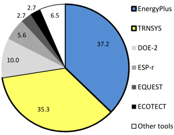
To provide an overview of building simulation programs used in optimization studies, this paper investigates the intensity of utilization of 20 major building simulation programs (among hundreds of tools3) as recommended in [40], including: EnergyPlus, TRNSYS, DOE-2, ESP-r, EQUEST, ECOTECT, DeST, Energy-10, IDE-ICE, Bsim, IES-VE, PowerDomus, HEED, Ener-Win, SUNREL and Energy Express (BLAST, TAS, TRACE and HAP were not included here due to irrelevant results). The search was performed on 2/4/2013 on Scopus – the world’s largest abstract and citation database of peer-reviewed literature4, using the keyword group [name of a program; optimization; building] for the period 2000 - 2013, then refining by some other keywords to eliminate irrelevant results. Figure 3 shows an approximation of the utilization share of the major building simulation programs. It is easy to find overwhelming shares of EnergyPlus, TRNSYS, DOE-2 and ESP-r among others. Possible explanations are likely to be the text-based format of inputs and outputs which facilitates the coupling with optimization algorithms and, of course, their strong capabilities as well. Interestingly, the utilization share of building simulation programs given by Google Scholar is quite similar to that shown in Figure 3.

3

There have been 395 building energy tools being listed at http://apps1.eere.energy.gov/buildings [Accessed 15/3/2013]

4

(9)

9

Table 4 alphabetically introduces a number of mostly-used optimization programs found in building optimization literature and their key capabilities. Some other optimization tools that have rarely been mentioned by the BPS community are Topgui, Toplight, tools on Java environment… From the result of an interview of 28 building optimization experts [15], it was found that GenOpt [2] and MatLab environment [41] are mostly-used tools in building optimization. GenOpt is a free generic optimization tool designed to apply to BOPs, thus it is suitable for many purposes in BPS with acceptable complexity. A limitation of the current GenOpt versions is that it does not have any multi-objective optimization algorithm. MatLab optimization toolboxes and Dakota [42] are not specifically designed for building simulation-optimization; thus these tools require more complex skills to use. However, the Neural Network toolbox in Matlab and the surrogate functions in Dakota do allow users to replace a computationally expensive model by a surrogate model. On the building optimization point of view, the free tool MOBO [43] shows promising capabilities and may become the major optimization engine in coming years. Some authors in [15] recommend modeFrontier (a commercial code) [44] for building optimization.

37.2 35.3 10.0 5.6 2.7 2.7 6.5 EnergyPlus TRNSYS DOE-2 ESP-r EQUEST ECOTECT Other tools

(10)

Citation: Nguyen, A. T.; Reiter, S.; Rigo, P. A review on simulation-based optimization methods applied to building performance analysis. Applied Energy 113 (2014) 1043–1058 Status: Postprint (Author’s version)

Name Open source? Multi-objective algorithm ? Parallel compu-ting? Handling discrete + continuous variables? Parame -tric study? Sensiti-vity analysis? Generic for BPS programs ? Multiple algori-thms? User inter-face? Cost function flexibi-lity? Parameter flexibility? Algori-thmic extensi-bility? Surrogate model? Operating system? Altair HyperStudy - + ? - + + + + + + + ? + Window BEopt + + + + + - - - + - +/- + - Window

BOSS quattro + + + + + + + + + + ? + + Unix, Linux, Window

DAKOTA + + + + + + + + + + + ? + Window, Linux

GENE_ARCH + + - - - - - + ? + + - - ?

GenOpt + - + + + - + + - + + + - Independent

GoSUM - - + + - + + - + + + ? + Window

iSIGHT - + - + + + + + + + + - - Window, Linux

jEPlus+EA + + + + + - - + + - + - - Independent

LionSolver - + - - - - + - + - - - + Window

MatLab toolbox - + + + + + + + +/- + + + + Window, Mac, Linux

MOBO + + + + - - + + + + + + - Independent

modeFRONTIER - + + + - + + + + + + ? + Window, Linux

ModelCenter - + + + - + + + + + + - - Window

MultiOpt 2 - + ? + - - - - + - - - - Window

Opt-E-Plus + + + + - - - - + - - + - Window

ParadisEO + + ? + - - + + - + + + - Window, Mac, Linux

TRNOPT - - - + + - - + + + + + - Window

“+” means Yes; “-” means No; “?” means Unknown

(11)

Citation: Nguyen, A. T.; Reiter, S.; Rigo, P. A review on simulation-based optimization methods applied to building performance analysis.

Applied Energy 113 (2014) 1043–1058

Status: Postprint (Author’s version)

5 Efficiency of the optimization methods in improving building

performance

It is important to know the capability of the simulation-based optimization method in improving design objectives such as indoor environment quality or building energy consumption. This allows designers to choose an appropriate method among a number of available approaches that can satisfy their time budget, resources and design objectives.

First, this work considers some studies in cold and temperate climate. In [13], the authors found that a reduction of 23–49% in the space heating energy for the optimized house could be achieved compared with the reference detached house. Most optimal solutions could be seen as Finnish low-energy houses. Similar to these results, Suh et al. [45] found 24% and 33% reduction of heating and cooling energy in a post office building in Korea using a knowledge-based design method and the simulation-based optimization method, respectively. By performing optimization on EnergyPlus models of an office floor under 3 climates of the U.S., Wetter and Wright [46] found a saving of an order of 7% to 32% of primary energy consumption, depending on the building location. In [47], optimal settings of optimization algorithms led to a reduction of 20.2% to 29.6% of the primary energy use by a large office building in temperate climates of the U.S. From these results, it is very likely that a reduction of 20% - 30% of building energy consumption is an achievable target using the building design optimization.

However, the situation of warmer climates is likely not the same. In a study related to a large office building, Kampf et al. [47] found a reduction of total energy consumption of 7.1% in a warm climate (Florida, U.S.). Nguyen [24] improved thermal comfort and energy consumption in 3 typical existing dwellings in 2 running modes under 3 hot humid climates by performing the optimization on calibrated EnergyPlus models. The optimal performances were compared with the references, giving a straightforward estimate of optimization efficiency. In average, the author found that discomfort periods in the naturally ventilated dwellings could be reduced by 86.1%, but the life cycle cost (50-year energy cost + construction cost) of the air-conditioned dwellings could only be reduced by 14.6%.

Cost reduction in optimization of high-performance buildings seems to be very minor. Salminen et al. [48] tried to improve energy consumption of a LEED-certified commercial building in Finland. They found that the optimization method could further reduce up to 10% of the annual energy consumption, accompanied by an additional investment of about 0.6 million Euros. Without the additional investment, improvement could only reach 1.1%.

Cost reductions by optimization methods clearly depend on the objective function to be minimized [24] and many other factors (climates, building models, optimization algorithms…). Due to very limited results from the literature and the variety of the design objectives in optimization studies, a robust quantification of optimization efficiency needs further investigations.

(12)

12

6 Challenges for simulation-based optimization in building performance

analysis

6.1 Handling discontinuous problems and those with multiple local minima In building design optimization, analysts must sometimes assign integer or discrete values to building design variables, which cause the simulation output to be disordered and discontinuous. Even with optimization problems where all inputs are continuous parameters, the nature of the algorithms in detailed building simulation programs itself often generates discontinuities in the simulation output [49; 32]. As an example, if the simulation program contains empirically assigned inputs (e.g. wind pressure coefficients), adaptive solvers with loose precision settings or iterative solvers using a convergence criterion (e.g. EnergyPlus program), simulation outputs are likely to be discontinuous. Such discontinuities can cause erratic behavior of optimization algorithms that result in failure or adversely affect on the convergence of the optimization algorithms [46]. Figure 4 shows an example of such discontinuities which caused the Hooke-Jeeves algorithm (a derivative-free optimization method) to stray away from the global minimum (at the lowest corner of the search space).

Other authors argued thatbuilding energysimulation programs can generally be seen as black-box function generators; thus gradient information that is required by several mathematical optimization methods is entirely unavailable[50; 51].Consequently gradient-based optimization algorithms, e.g. Discrete Armijo Gradient algorithm [52], are not recommended for solving BOPs. On the other hand, a simulation program may employ iterative or heuristic solvers, low-order approximations of tabular data, or other numerical methods which produce noise to simulation outputs [51]. Thus the objective functions in BOPs are generally multi-modal and discontinuous (thus non-differentiable). Some optimization algorithms may fail to draw a distinction between a local optimal solution and a global one (or fall into a trap by a local one), and consider the local optimum as the final solution to the problem. An example is shown in Figure 5 which shows a possible failure of Figure 4: Discontinuity in energy consumption as a function of east and west window configurations. The dots show the optimization process of the Hooke-Jeeves algorithm [32]

(13)

13

the Simulated Annealing algorithm (due to inappropriate settings of the algorithm) in solving a multi-modal function.

This raises a question of whether an optimization algorithm is suitable for the BOP at hand and how to define correct settings of both the optimization algorithm and the precision of simulation programs. Efficient and powerful search methods are obviously needed to explore such building problems. New simulation tools should be programmed such that the precision of solvers which are expected to cause large discontinuities in the outputs can be controlled [46]. Several numerical experiments [5; 46] have indicated that the meta-heuristic search method should be the first choice for BOPs. However, in large-scale BOPs this method does not guarantee optimal solutions to be found after a finite number of iterations.

6.2 Performance of optimization algorithms and the selection

The demand of a search-method that works efficiently on a specific optimization problem has led to various optimization algorithms. As a result, the choice of optimization algorithms for a specific problem is crucial to yield the greatest reduction [54]. The problem of how to select an optimization method for a given BOP is not trivial and usually based on a number of considerations [2; 50]:

- Natures of design variables: continuous variables, discrete variables or both; - The presence of constraints on the objective function;

- Natures of objective functions (linear or nonlinear, convex or non-convex, continuous or discontinuous, number of local minima, etc.)

- The availability of analytic first and second order derivatives of the objective functions;

- Characteristics of the problem (static or dynamic…);

- Performance of potential algorithms which have similar features.

Providing a generic rule for the algorithm selection is generally infeasible due to the complexity and the diversity of real-world BOPs. However, by using the data from the literature related to building optimization, the trend of use of optimization algorithms can be estimated (see Figure 6). It can be seen that the stochastic population-based algorithms (GAs, PSO, Hybrid algorithms, evolutionary algorithms) were the most frequently used methods in building performance optimization. Such stochastic algorithms cannot guarantee that the best solution will be reached after a finite number of iterations, but they are used to obtain good solutions in a reasonable amount of time [44].

Figure 5: If the temperature is very low with respect to the jump size, Simulated Annealing risks a practical entrapment close to a local minimum (adapted from [53])

(14)

14

There are a number of reasons that makes the GA popular among BPS communities: - Capability of handling both continuous and discrete variables, or both types; - Concurrent evaluation of n individuals in a population, allowing parallel

simulations on multi-processor computers;

- Working with a population of solutions makes GA naturally suited to solve multi-objective optimization problems [55];

- Robust in handling discontinuity, multi-modal and highly-constrained problems without being trapped at a local minimum; even with NP-hard problems [56]; - Robust to high simulation failure rates, as reported by J. Wright in [15].

The performance of optimization algorithms in solving BOPs was the interest of many researchers. It is sometimes considered as a criterion for selecting an optimization algorithm. Wetter and Wright [46] compared the performance of a Hooke-Jeeves algorithm and a GA in optimizing building energy consumption. Their result indicated that the GA outperformed the Hooke-Jeeves algorithm and the latter have been attracted in a local minimum. Wetter and Wright [5] compared the performance of 8 algorithms (Coordinate search algorithm, HJ algorithm, PSO, PSO that searches on a mesh, Hybrid PSO-HJ algorithm, Simple GA, Simplex algorithm of Nelder and Mead, Discrete Armijo gradient algorithm) in solving simple and complex building models using a low number of cost function evaluations. They found that the GA consistently got close to the best minimum and the Hybrid algorithm achieved the overall best cost reductions (although with a higher number of simulations than the simple GA). Performances of other algorithms were not stable and the use of Simplex algorithm and Discrete Armijo gradient algorithm were not recommended. Kampf et al. [47] compare the performance of two hybrid algorithms (PSO-HJ and CMA-ES/HDE) in optimizing 5 standard benchmark functions (Ackley, Rastrigin, Rosenbrock, Sphere functions and a highly-constrained function) and real-world problems using EnergyPlus. They found that the CMA-ES/HDE performed better than the PSO-HJ in solving the benchmark functions with 10 dimensions or less. However, if the number of dimensions is larger than 10, the PSO-HJ worked better. Both these algorithms performed well with real-world BOPs on EnergyPlus models. Hamdy et al. [39] tested performance of three multi-objective algorithms, NSGA-II, aNSGA-II and pNSGA-II, on a BOP and 2 benchmark test problems. They reported that the aNSGA-II found high-quality solutions close to the true Pareto front with fewer evaluations and achieved better convergence.

8 1 1 1 1 1 2 2 2 2 4 5 5 10 13 40 0 5 10 15 20 25 30 35 40 Other

Harmony search algorithms Coordinate search algorithms Simplex algorithms Discrete Armijo Gradients …

Tabu search Branch and Bound methods Other direct search algorithms Ant colony algorithms Simulated annealing Other evolutionary algorithms Hooke-Jevees algorithms Linear programing methods Hybrid algorithms (all types) Particle swarm optimization Genetic algorithms

Use frequency (times)

Figure 6: Use frequency of different optimization algorithms, the result was derived from more than 200 building optimization studies given by SciVerse Scopus of Elsevier

(15)

15

Elbeltagi et al. [57] compared performance of 5 evolutionary-based optimization algorithms, including GAs, memetic algorithms, particle swarm, ant-colony systems, and shuffled frog leaping, in solving benchmark functions and project management problems. They found that the behavior of each optimization algorithm in all test problems was consistent and that the PSO algorithm was likely to perform better than the others in terms of success rate and solution quality, while being second best in terms of processing time.

Hybrid algorithms (e.g. PSO-GPS [2], GA-GPS [58] or CMA-ES/HDE [47; 59]) shows a remarkable capability in dealing with discontinuous, highly constrained mixed-integer and/or multi-modal problems as frequently observed in building simulation outputs. The hybrid algorithms have been implemented in some computer programs (e.g. GenOpt, Matlab optimization toolbox…) that can be applied to building performance analysis. In GenOpt [2], Wetter introduced the Hybrid algorithm PSO-HJ in which the PSO is performed the search on a mesh, significantly reducing the number of cost evaluations called by the algorithm [60].

In [5; 47] optimization results have also indicated that the cost reduction by an algorithm not only depends on the natures of the algorithm, but also depends on the settings of algorithm parameters. It is necessary to stress that according to the so-called ‘no free lunch theorem’ [61], there is no single best algorithm for all optimization problems. Hence, algorithm selection and settings might involve trial and error.

6.3 Multi-objective building optimization problems

About 60% of the building optimization studies used the single-objective approach, e.g. only one objective function can be optimized in an optimization run [62]. However, in real-world building design problems designers often have to deal with conflict design criteria simultaneously [18; 63] such as minimum energy consumption versus maximum thermal comfort, minimum energy consumption versus minimum construction cost… Hence, multi-objective optimization is, in many cases, more relevant than the single-objective approach.

There have been several methods to solve a multi-objective problem. The most simplistic approach, known as “scalarization”, is to assign different weight factors to each criterion, and then the objective function will be simply the weighted sum of the criteria [64]. As an example, the multi-objective optimization will turn into a single-objective problem by the linear scalarization as follows:

1 min ( ) n i i x X i w f x ∈

∑

₌ (1)

where wi is weight factor of the ith objective function (wi > 0).

The new objective function is a scalar measure. As an example, we consider an optimization problem of a thermal zone which consists of a construction cost function fc(X)

and a comfort performance function fp(X). These functions could be integrated into a single

objective function by assigning two weight factors (w1 and w2):

1 2

( )

_c

( )

_p

f X

=

w f X

+

w f X

(2)

Wang et al. [65] simultaneously optimized 3 objective functions using 3 equal weight factors to find optimal configurations of a building cooling – heating and power system. A drawback of this approach is the difficulty in estimating the weight factor wi

because objective functions do not have the same metric or the same significance. In addition, the optimization can only give a unique optimal solution. Anyway, an estimate of the Pareto front can be achieved by running the optimization several times with different weight factors.

(16)

16

Another approach is to use the concept of Pareto optimality in which a set of trade-off optimal solutions (a Pareto set) is examined and appropriate solutions are then determined. This approach is referred to as “multi-objective optimization” or “Pareto optimization”. For any given problem, the Pareto optimal set can be constituted by an infinite number of Pareto points. Pareto optimization strategies are, in most cases, aimed to provide only some elements of the Pareto set rather than the entire one. Due to the complexity of BOPs, researchers often use up to two objective functions, but a very few exceptions with 3 or more functions have been observed as shown in [37] (three objective functions were indoor environment quality, the carbon payback period, and cash payback period time), in [66] (energy consumption, CO2 emission and initial investment cost) or in

[38] (energy consumption, thermal comfort and initial investment cost).

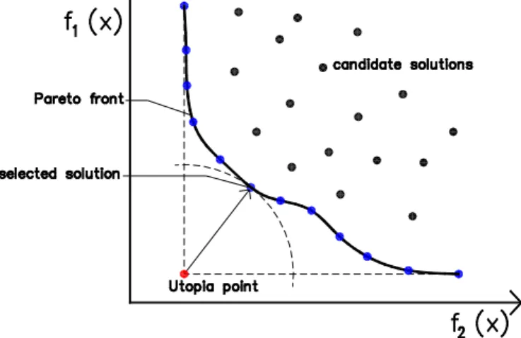
The problem of how to select the best solution from the Pareto set is not trivial as it depends on a number of aspects (e.g. the significance of objective functions, the demand of building investors…). This process is known as multi-criteria decision making. Many decision making techniques have been developed [67] such as “pros and cons”, “simple prioritization”, “satisficing”, “opportunity cost”, “bureaucratic”. Figure 7 presents a common strategy in engineering applications to select the best solution among the Pareto set if two objective functions are equally important.

Although many Pareto optimization strategies have been developed as reviewed in [4], the multi-objective optimization with the GA seems the mostly used strategy in building performance analysis, for example multi-objective 3-phase GA in optimizing a detached dwelling [63], NSGA in [20; 27], MOGA in optimizing a green building model [16], NSGA-II in optimizing cellular fenestration on building façades [68]. Being a population-based method, GAs are well suited to solve multi-objective optimization problems. A number of GA-based multi-objective optimization methods as been developed as reported in [69] among which the Vector evaluated GA (VEGA) [70], Multi-objective Genetic Algorithm (MOGA) [71], Niched Pareto Genetic Algorithm (NPGA) [72], Weight-based Genetic Algorithm (WBGA) [73], Non-dominated Sorting Genetic Algorithm (NSGA) [74], Fast Non-dominated Sorting Genetic Algorithm (NSGA-II) [75], Multi-objective Evolutionary Algorithm (MEA) [76] are frequently used in building research. Sometimes, strategies other than the GA was used such as Multi-objective Particle Swarm Optimization (MOPSO) in optimizing thermal comfort and building energy consumption [77], Multi-objective Ant Colony Optimization (MACO) in optimizing building life cycle energy consumption [78]. As being observed from these studies, the used methods aim at producing

(17)

17

a representative subset of the Pareto optimal set from which decision-makers can derive the most appropriate solution to the problem at hand.

At present, there are some programs that provide the platforms for multi-objective optimization such as Matlab [41] optimization toolbox (with a MOGA algorithm); modeFRONTIER [44] (with a MOGA-II, an Adaptive Range Multi-objective Genetic Algorithm – ARMOGA, a Multi-objective Simulated Annealing – MOSA, a NSGA-II, a Fast Multi-objective Genetic Algorithm – FMOGA, a Multi-objective Game Theory – MOGT, a MOSPO); LionSOLVER [79] (with multi-objective Reactive search optimization); Dakota [42] (with a MOGA algorithm and a scalarization method); a revised GA implemented in GenOpt by Palonen et al. [58]; Multiopt2 [38] (with NSGA-II), MOBO [43] (with NSGA-II, Omni-optimizer, Brute force, random search).

6.4 Issues related to optimization design variables

The number of independent variables in the optimization is not restricted by most optimization algorithms, but should be limited on the order of 10 [2]. Figure 8 shows a statistical result of the number of optimization variables derived from 10 arbitrary studies [63; 80; 30; 81; 22; 20; 5; 18; 16; 54]. In average each optimization study used 15.1 variables with a fairly high standard deviation of 5.6 (max = 24, min = 8). The number of independent variables is obviously dependent on the capability of the optimization algorithm and the complexity of the problem. However, an appropriate number of independent variables for a building optimization problem (BOP) are still subject to debate and further investigations on this topic are therefore needed.

In ‘real-world’ BOPs, analysts sometimes have to deal with problems that have both discrete variables (e.g. building components) and continuous variables (e.g. design parameters). For example, the decision variable X1 of the night ventilation scheme must be

either 1 or 0 in any optimal solution, modeling a yes/no decision and X1 is called a binary

integer variable. Such problems are referred to as a “Mixed-Integer Programming” problem. Discrete variables generally make the optimization problem non-convex and discontinuous, and therefore far more difficult to solve [82; 83; 51]. Memory and computational cost may rise exponentially as more discrete variables are added in the problem [82]. Stochastic population-based algorithms (e.g. GA, evolutionary algorithms), which randomly generate and improve a population of candidate solutions, may satisfy the mixed-integer problem in optimization. Nevertheless, these methods are generally not able to assure “optimality” of the solution. It is generally recommended that discrete variables should be avoided by all possible means in optimization [84].

0 5 10 15 20 25

Hamdy et al. (2011a) Holst (2003) Tuhus-Dubrow & Krarti (2010) Suga et al. (2010) Hamdy et al. (2011b) Evins et al. (2012) Wetter & Wright (2004) Fesanghary et al. (2012) Nguyen & Reiter (2013) Wang et al. (2005)

Continuous variable Discrete variable

(18)

18

Constraints imposed on both independent and dependent variables are usually formulated in form of functions of these variables, e.g. x₁+x₂ ≤1. Variables’ bounds constitute a particular case of the more general constraints. For dependent variables’ constraints, most optimization algorithms force users to define constraints by using penalty or barrier functions, but some optimization tools and algorithms are able to handle constraints separately and automatically (e.g. Matlab optimization toolbox, MOBO [43], CONLIN method [85]…). Sometimes, a BOP may have "higher-level" constraints, e.g. the constraints that require a set of independent variables to be of non-repeating ordering integers - from 1 to n (as in traveling salesman problem). In building research, such a constraint type may occur, such as in optimization of heating systems where the choices of boiler types (A, B, C, D) and fuel options (gas, diesel, biomass, district heating) are mutually accepted or excluded.

Constraints and "higher-level" constraints on both dependent and independent variables are often unavoidable in a BOP, but they often make the optimization problem more difficult to solve, especially equality constraints [86]. It is recommended that an equality constraint should be converted into an in-equality constraint where possible [14].

In [64] the authors imposed 12 constraints on the optimization of an HVAC system, including 6 coil design constraints, 4 fan envelope constraints, and 2 setpoint constraints. Nguyen [24] imposed a special thermal comfort constraint on the cost function as follows:

(

)

2 max ( ) ( ) f xc 10 max 0, %( ) 10 f x TDH x COST +  −  ≜ (3)

where fc(x) is construction cost; COSTmax is maximum construction cost; TDH%(x)

is the total discomfort hours/year, must be smaller than 10%. Each time thermal comfort is violated, the penalty function (the rightmost term of equation (3)) will add a large positive term to the objective function.

In order to maintain a reasonable number of design variables in the optimization, sensitivity analysis may be performed to screen out insignificant variables. Several sensitivity analysis techniques can be used such as local sensitivity analysis methods, screening methods, Monte Carlo-based methods, variance-based methods or “design of experiment” methods. Due to the complexity of detailed building simulation programs, simulation outputs are generally nonlinear, multi-modal, discontinuous [32; 5], non-monotonic [87] and may contain both continuous and discrete variables, global sensitivity analysis rather than local one should be used. The Morris’s method, Sobol’s method and regression-based sensitivity indices seem to be the mostly-used measures of sensitivity [10; 88; 24; 89]. Tian [90] provides a good review of sensitivity analysis methods applied to building energy analysis. Evins et al. [20] used a full-factorial DOE method to select influential factors of the design of a flat in UK for the optimization phases. They could obtain 21 highly significant variables among more than 100 design variables. Nguyen [24] used the Monte Carlo-based method and regression-based sensitivity indices to reduce the number of optimization variables to nearly a half. Figure 9 shows an example of sensitivity order of design variables from which significant variables were derived for the subsequent optimization. Although many commercial programs can perform sensitivity analysis, the authors recommend SimLab program [91] and Dakota [42] (free of charge) for such a task in BPS.

(19)

19

6.5 Optimization of computationally expensive models

Simulation of detailed building models may take several minutes in building energy simulation [27] to several hours in computational fluid dynamics (CFD) simulation [92] to complete while the simulation-based optimization techniques often require hundreds or thousands of simulation evaluations. The optimization schemes may therefore become infeasible due to such computationally expensive building models. To overcome this, very simplified models instead of detailed building models can be used, as in [34; 93; 65]. This method has many limitations such as incapability in modeling complex building systems and phenomena, thus it is only suitable for research purposes. Particularly, in [21] Lee used a two-step optimization scheme to deal with his expensive CFD model. In the first step, Lee performed the optimization on the simple CFD model. Then he performed a few detailed CFD simulations on the optimal candidate solutions found in step 1 to refine the results. Other methods can be employed by reducing the population size and/or the number of generations. However, these reductions significantly lower the performance of optimization algorithms, possibly resulting in sub-optimal solutions [16]. In 1986, Fleury and Braibant [85] propose the CONLIN method that can deal with expensive structural models by replacing the primary model with a sequence of explicit approximate sub-problems by performing linearization. These explicit sub-problems are convex and separable, thus can be solved efficiently by using a dual method approach [94]. Consequently, the CONLIN method can handle mixed-integer and/or non-differential, computationally expensive problems as described in [95].

Surrogate models are among promising solutions to this problem. A surrogate model (meta-model or emulator) is an approximation model of the original simulation model. It typically mimics the behavior of the original model to be able to produce the model responses at reduced computational cost.

Establishing a surrogate model often goes through 3 major steps as follows:

-0.2 -0.15 -0.1 -0.05 0 0.05 0.1 0.15 0.2 0.25 Length of window overhang

South windows’ height North windows’ height West windows’ height Brick density (external wall) Max equipment power -kitchen Insulation thickness ground floor Crack of the roof Max equipment power – all zones Thickness wooden floor Crack window - bedrooms Conductivity EPS insulation Thickness of internal partitions Thickness - brick Density ceiling concrete slab Window type Thickness of internal mass Max number of occupant East windows’ height Discharge coeff. other rooms Roof color Thickness roof insulation Crack window – other rooms Thickness ceiling concrete slab Discharge coeff. bedrooms Power of gas stove External wall type Ventilation strategy External wall color

SRRC ranking

Figure 9: Sensitivity ranking of design variables by Standardized Rank Regression Coefficient (SRRC) (adapted from [24])

(20)

20

- Sampling input vectors and calculating corresponding model responses, which constitute a database for training a surrogate model.

- Constructing the surrogate model based on the database by selecting an appropriate method, e.g. Kriging, Support vector machine, artificial neural network (ANN).

- Validating the model before being used as a “surrogate” of the original model. The second and the third steps may be repeated iteratively until the validation achieves success. In the context of optimization, surrogate models can speed convergence by reducing function evaluation cost and/or smoothing noisy response functions [42; 51] which are problematic in BOPs. After running the surrogate-based optimization, other refined optimization around the optimal points using the original model can be performed to obtain exact solutions. The most common strategy of the surrogate-based optimization method is presented in Figure 10.

In some computer programs (e.g. MatLab [41], Dakota [42], modeFrontier [44]), several surrogate model choices are possible, which are categorized as response surface methods, data fits, multi-fidelity models, and reduced-order models, ANNs, Bayesian networks...

In 2000, Klemm et al. [96] showed a pioneer effort in surrogate-based optimization by applying a polynomial regression method on CFD simulation results to derive explicit analytic objective functions, then optimizing them using a simple deterministic optimization method. Magnier and Haghighat [27] used TRNSYS simulations to train an ANN, then used the trained - validated ANN to couple with the GA to optimize thermal comfort and energy consumption. The database for training the ANN consists of output of 450 simulations. Time for generating the database was 3 weeks, but optimization time was very small. If direct coupling between TRNSYS and GA was used, it would need 10 year to finish the task [27]. Chen et al. [26] used a feed forwards neural network with one hidden layer for the identification of temperature in intelligent buildings and then optimize by the PSO. Eisenhower et al. [23] used the Support Vector Machines method to generate several meta-models of a 30-zone EnergyPlus building model and then performed sensitivity analysis to select the most influential variables for optimization. The database used to generate the meta-models consists of 5000 simulated solutions. These authors stated that the optimization using the meta-model offers nearly equivalent results to those obtained by EnergyPlus model. Tresidder et al. [97] used Kriging surrogate model to optimize building CO2 emission and construction cost, and then compare the results against those given by the

GA on the same design problem. They stated that the Kriging surrogate models was able to Figure 10: Surrogate models applied to building simulation - optimization

(21)

21

find the optimum in fewer simulation calls than the stand-alone GA and could find a better trade-off if the number of simulations was restricted. They also recommended that the use of Kriging models for optimization of complex buildings requires further investigations. In [92], Khan et al. used the “moving least squares method” to establish a surrogate model from extremely expensive CFD simulations, then optimized the design of a ventilation system in hospital wards by this surrogate model. Gengembre et al. [98] minimize 20-year life cycle cost of a single-zone building model using a Kriging surrogate model and the PSO. They concluded that the accuracy of their Kriging model is acceptable and such a surrogate model can further help designers in design space exploration with cheap simulation cost.

The problem of sensitive objective function (a small deviation from the optimum variables can result in significant degradation of the objective function value) makes surrogate models (e.g. models by the ANN) possibly irrelevant in some optimization situations (see Figure 11). It is necessary to note that the use of a surrogate model instead of an ‘actual’ building model increases the uncertainty and the risk of accumulative errors in the whole optimization process. The accuracy and sensitivity of surrogate-based optimization is currently not a well-developed area, especially when the number of input variables is large [14], the cost function is highly discontinuous or in cases many discrete input variables exist.

The strength and weakness of various surrogate methods is a great research field of computational and statistical science and well beyond the scope of the building simulation community. At present, there is no consensus on how to obtain the most reliable estimate of accuracy of a surrogate model, thus the correlation coefficient R² is often applied, as in [27; 29]. Furthermore, the random sampling method of inputs, the number of building model evaluations used to construct and validate a surrogate model is still problematic and is often chosen empirically by analysts. It also needs more studies to see whether significant difference between optimization results given by a surrogate model and an ‘actual’ building model exists. These questions are explicitly challenges of the building research community.

6.6 Building design optimization under uncertainty

In optimization building design using simulation approaches, analysts often have to deal with uncertainty during various steps of the optimization, resulting in uncertain optimal solutions. The uncertainty may arise from design variables, the climate, building operation, building performance assessment criteria, noise in cost function evaluations by computer programs, vagueness in variables constraints, etc [36; 14]. Thus, optimal solutions must not only satisfy the requirement of building performance but also be robust to small deviations of optimization inputs and constraints. Such a task is referred to as “robust design optimization” (RDO). RDO is defined as a methodology to optimize the design which is insensitive to various variations [99] (e.g. environment, systems or models). A simple illustration of this concept is explained in Figure 11. Instead of looking for the sensitive global optimum x1, one should find the local, but robust optimum x2. The performance of

(22)

22

Unlike deterministic optimization, in RDO one has to deal with the probabilistic functional of the objective functions. The model outputs are usually represented in terms of moments like “mean” and “standard deviation” [44]. The simplest mathematical formulation of a RDO problem can be written as follows:

find X to minimize:

( , ) ( _f( , ), _f( , ))

f X pɶ =F

µ

X p

σ

X p (4)

subject to: g(X,p) ≥ 0 and/or h(X,p) = 0; where

X = (x1, x2, …, xn) is a design variable vector, subject to

l u

i i i

x

−∞ ≤

≤ ≤

≤ +∞

; p is

a system constant parameter vector (both X and p could be uncertain);

µ

_f

( , )

X p

and

( , )

f

X p

σ

are the mean and standard deviation functions of the original objective function f(·) under uncertainty variations of X and p; F(·) is the reformulated optimization objective function with respect to

µ

_f

( , )

X p

and

σ

_f

( , )

X p

.

Equation (4) means to find a solution that provides lowest mean cost function and minimum standard deviation simultaneously. The simplest method for solving the problem (4) is to apply two weight factors (as introduced in equation (2)) on

µ

_f

( )

X

and

σ

_f

( )

X

functions, then treat the function F(·) as a single-objective optimization problem. This method is sometimes applied to building studies, as in [100; 101]. For more sophisticated approaches, readers are asked to refer to [99].

Pioneer studies on optimization under uncertainty can be traced back to the 1950s [102]. Since then this research field has become a “fertile ground” for researchers as reviewed in references [103; 99]. To accurately evaluate the robustness of candidate solutions with respect to uncertainties, a significant amount of extra function evaluations is needed [104]. Building optimization problems are inherently difficult and time-consuming, and they generally become even more difficult due to additional efforts to deal with these uncertainties, that may result in significant computational burden. It is therefore essential to filter out low influential inputs and simplify the RDO by using sensitivity analysis [24; 23; 20]. Another method is to use surrogate models (meta-models) to replace computationally expensive real building simulation models in RDO.

By testing on 6 benchmark functions, Kruisselbrink, et al. [104] found that the Kriging-based method for finding robust optima outperformed the tested benchmark methods (single evaluation and multi evaluation method) proposed by other authors. Hopfe Figure 11: Sensitive and robust optimal solutions of a single-variable function (adapted from [100])