1
Regulatory Incentives to Water Losses Reduction:
The case of England and Wales
Brea-Solis, Humberto*; Perelman, Sergio+; Saal, David †
*Université Côte d’Azur, SKEMA +University of Liege (ULg), HEC Management School,
† Loughborough University
Abstract
In recent years, England and Wales have suffered droughts. This unusual situation defies the common belief that the British climate provides abundant water resources and has prompted the regulatory authorities to impose bans on superfluous uses of water. Furthermore, a large percentage of households in England consume unmetered water which is detrimental to water saving efforts. Given this context, we estimate the shadow price of water using a panel data from reports published by the Office of Water Services (Ofwat) for the period 1996 to 2010 (three regulatory periods). These shadow prices are derived from a parametric multi-output multi-input input distance function characterized by a translog technology. Following O'Donnell and Coelli (2005), we use a Bayesian econometric framework in order to impose regularity – monotonicity and curvature – conditions on a high-flexible technology. Consequently, our results can be interpreted at the firm level without requiring the need to base analysis on the averages. Our estimations offer guidance for regulation purposes and provide an assessment of how the water supply companies deal with water losses under each regulatory period. The relevance of the study is quite general as water scarcity is a problem that will become more important with population growth and the impact of climate change.
Keywords: Water supply, Regulation, Shadow Prices, Bayesian Econometrics JEL: L51, L95, C11, D24
Acknowledgment: Humberto Brea-Solís and Sergio Perelman acknowledge financial support from the Fonds de la Recherche Scientifique FNRS (FRFC Project Beyond Incentive Regulation). We thank Luc Bauwens, Chris O’Donnell, and Phillippe Lambert for very helpful conversations and advice on Bayesian estimation issues and the two anonymous referees for their suggestions and commentaries that helped us improve the paper.
2 1. Introduction
According to the UN fact sheet about water, 1.8 billion people will be living in countries with absolute water scarcity and two-thirds of the world’s population could be under stress conditions in 2025. Furthermore, severe weather fluctuations between droughts and wet periods are not only affecting regions where these problems are prevalent but also nations like the United Kingdom (UK), that traditionally have been perceived as rainy countries with abundant water resources. In particular between the years 2010 to 2012, the UK suffered a harsh drought that prompted the regulatory authorities to impose bans on superfluous uses of water. Conversely, the winter season that ended in 2014 has been the wettest since 17661.
Extreme weather conditions jeopardize continuity of supply. Therefore, it is essential that regulators incentivize an efficient use of water resources. England and Wales have the additional complication that only a small percentage of households have metered water services. Most of the customers pay a fixed amount according to the rateable value of their property. This feature discourages efforts to save water from both consumers and companies.
In this study we estimate the shadow price of water, which is the implicit value assigned by the companies to this precious resource. The computation of shadow prices provides valuable information in the context of non-marketable goods and in particular for the internalization of negative externalities. According to Dang and Mourougane (2014), an accurate measure of shadow prices could help policymakers in three ways: (1) regulators could compare the private cost of internalizing the externalities with the marginal benefits of the environmental protection before determining the regulatory scheme; (2) they can be used as a reference point or benchmark to set penalties or taxes for not complying with the environmental targets and (3) shadow prices are useful for adjusting gross domestic product and productivity indexes used in long-term analysis. Furthermore, comparing shadow prices of non-marketable goods with prices of similar marketable goods (e.g. van Soest, List and Jeppesen, 2006; Fare, Grosskopf, Noh and Weber, 2005) provide insight about the current incentive structure of the industry. In our context, the shadow price of water can be compared to the prices charged per cubic meter of water delivered (for metered households) to determine if water suppliers have appropriate incentivize to increase profits by reducing leakage. However, given strong regulatory incentives to improve cost-efficiency, water
1 Met Office website: http://www.metoffice.gov.uk/news/releases/archive/2014/early-winter-stats. Accessed
3
suppliers might also forgo costly leakage reduction efforts in order to avoid being penalized for not achieving cost efficiency targets.
In our study, shadow prices are estimated using the Bayesian econometric methodology proposed by O’Donnell and Coelli (2005). The first step is the calculation of an input distance function with a translog functional form that complies with homogeneity, monotonicity and curvature restrictions. Afterwards the shadow prices are computed and analysed. As discussed below, the selected approach follows the trend in the literature of treating a bad output as an input, which is more intuitive, if we consider the trade-off between a negative externality and investment in environmental friendly technologies and practices.
The panel data used in the analysis came from reports published by the Office of Water Services (Ofwat) for the period 1996 to 2010 and covers three regulatory periods (1996-2000, 2001-2005 and 2006-2010). In addition to the inputs and outputs, we control for other factors such as water quality, pressure, water source, unmetered households and whether the company is also engaged in sewerage related activities.
The paper has five sections in addition to the introduction. In the second section, we provide a brief background of the problem and the literature. The third section contains an explanation of the chosen methodology. The analysed dataset is described in the fourth section of the paper. We discuss the results in the fifth section and state our conclusions in the sixth.
2. Background
The water sector is considered a network industry. Shy(2001) indicated four characteristics of a network industry: 1) it provides a system (individual parts of the product or service do not satisfy customers’ needs); 2) it produces network externalities; 3) there are switching costs and lock-in and 4) the production displays significant economies of scale. Such network industry features create entry barriers that foster the formation of natural monopolies. The presence of natural monopoly suggests efficiencies in production by a single monopoly firm, and traditionally, water along with most utility sectors was treated accordingly, with two main policy solutions. One solution is the public provision of the goods or services required by society. The other solution is allowing private firms to satisfy the market’s needs while keeping these firms heavily regulated to prevent abuse of the firms’ monopoly power.
4
In the past 30 years, the tendency followed by governmental authorities is the privatisation of network industries, coupled with the vertical separation of a regulated natural monopoly network from potentially competitive upstream and downstream components. Thus, this approach has been applied in the UK, with varying degrees of success, in the rail, electricity, gas, and telecoms sector. In contrast, when the water and sewerage sector of England and Wales, was privatized in 1989, no attempt was made to introduce competition, and no vertical restructuring occurred. This was because it was generally accepted that considerable cost economies accruing from economics of scale and scope, thereby favouring a single integrated natural monopoly provider.2 Thus, the main goal of UK water privatization
was to improve the performance of the industry by providing improved incentives for cost efficiency via the implementation of price cap regulation (DOE, 1986). This decision has inspired several studies about the effectiveness of privatization and price cap regulation in these regions (Saal & Parker, 2000, 2001; Saal, Parker & Weyman-Jones, 2007; Bottasso & Conti, 2009a). The results of these studies show that privatization and the introduction of price cap regulation failed to robustly deliver the expected results and may have created incentives for opportunistic behaviour with respect to the cost cutting activities.
UK water privatization also had an important effect on quality, and was also partially motivated to facilitate private investment flows needed to improve the quality of service, which had suffered from underinvestment before privatisation (Saal & Parker, 2001) However, as there is a well known trade-off between producing quality goods and services and seeking cost-efficiency, the English and Welsh water regulator also modified the conventional price cap regime in order to counterbalance the tendency of neglecting quality. Specifically, a Q factor was included in the price cap formula for encouraging capital investment to comply with higher quality standards. Previous research suggests that this alteration implied a lax application of regulation in the first years after privatization and apparently an overinvestment in capital by the regulated firms (See Saal et al. 2007).
Moreover regulators primarily concentrated their efforts on the chemical properties of the water delivered, and customer observable characteristics such as customer pressure and call waiting times for customer service. Thus, the verification of the compliance of water
2 Recently the Water Service Regulation Authority (Ofwat) has promoted efforts towards introducing
competition in the retail provision of water supply in England and Wales, with such competition first being allowed in April 2017 for business customers only, but not for households. However, the extent of perceived cost benefits from natural monopoly benefit is still evident, as the new market structure will see water retailers simply reselling outputs provided by fully integrated and regulated wholesale services, who will provide all services except retail billing, account handling, metering, customer queries, and provision of water efficiency advice to consumers. Moreover, this reform falls well after the end of our sample period.
5
quality standards is performed by the Drinking Water Inspectorate (DWI) in England and Wales. In 2012, this entity published several reports addressing the quality standards for these regions in 2011. This documents show that water quality standards have improved since 1991. In letters addressed to the Ministers of England and Wales it was stated that in 2011 “[c]ompliance with the EU Drinking Water Directive for England and Wales combined was the same as the previous year at 99.96% with only 0.04% of 1.9 million tests failing to meet one of the chemical or microbiological standards”3. Similarly, the customer observable
characteristics of water supply monitored by Ofwat, have also shown considerable improvement since privatisation.
However, given increasing concerns with regard to water scarcity, it is notable that water losses have not received the same degree of attention since privatisation. 4 Nevertheless,
there is a confluence of factors that makes water losses relevant in England and Wales. First, the regions of England and Wales have suffered from droughts recently. According to the data included in the HadUKP UK Precipitation Dataset, 2011 was one of the driest years in England. The Met Office annual report state that East Anglia and Lincolnshire underwent severe drought only comparable to what happened in 1921 (Met Office, 2012). The beginning of 2012 followed the same trend as in 2011 prompting some water companies to impose a hosepipe ban in early April (The Guardian, 2012). After record precipitation during the following months, (e.g. April 2012 was the wettest month since the authorities started keeping records) the hosepipe ban was lifted by all companies in July 2012. Nevertheless, some companies caution that the threat of dry winters is not over (BBC, 2012). In addition, 2006, 2011 and 1999 presented the highest yearly average temperatures recorded in central England since they started being registered in 1659 according to the Hadley Centre Central England Temperature (HadCET) dataset. Studying the reasons behind this “climate change” go beyond the scope of this study. We will simply assume as an accurate assessment of reality that for some reason the levels of precipitation are declining and that temperatures are rising.
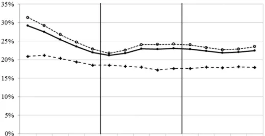
Moreover, despite the seriousness of extreme weather events, leakage remains a problem in the UK, and is very high by international standards. Figure 1 illustrates the percentage of leakage with respect to the total water distributed from 1996 to 2010. This timespan covers three regulatory periods (1996-2000, 2001-2005 and 2006-2010). There was
3 Letter addressed to John Griffiths AM, Minister for the Environment and Sustainability from the Drinking
Water Inspectorate DWI on July 3rd, 2012. The letter was published in the website of DWI.
http://dwi.defra.gov.uk/about/annual-report/2011/letter-wales.pdf accessed on September 7th, 2012.
4 Water losses or water leakage is defined as the water lost in the distribution process excluding losses within
6
only a substantial reduction of water leakage in the first regulatory period, and this was due to the imposition of mandatory targets to water companies by the authorities. This decision was a consequence of a severe drought in 1995 (Office of Water Services, 2000) and was not continued after the first five years of application. Afterwards leakage still remained at a high level with respect to other similarly developed countries like Germany and France. Figure 1 also reveals that companies that only produce water (Water only companies, WoCs) had a much lower level of leakage than companies that also handle sewerage services (Water and sewerage companies, WaSCs). Thus, despite, privatisation, the imposition of price cap regulation, and considerable efforts to improve the quality of water services, water losses continues to be high, and this situation has not prompted a n enduring regulatory response.
INSERT FIGURE 1
The potential ability to meet the challenge of increasing water scarcity is not only restricted by issues on the supply side but also relates to demand side issues. Projections for England and Wales elaborated by the Office of National Statistics suggest significant increases in population in coming years. |Thus, the combined population of England and Wales is estimated to increase from 56.1 million people in 2012 to 64.4 million in 2032. The population would increase 14.8% in 20 years, on average 0.7% per year (Office of National Statistics, 2012). Therefore, water companies face not only increased potential for droughts but also increasing population demand. To complicate things even further a large percentage of the English and Welsh households are not metered. According to the Position Statement of the Environmental Agency (2011), the average percentage of metered households in England and Wales is 35%. Hence, most of the customers do not pay for any water losses in their premises, and generally have little to no incentive to reduce water usage.
The UK is, of course, not the only country facing pressure to reduce water losses. Other countries are dealing with similar issues. Nevertheless, we have found very few papers analyzing water losses from an economic perspective. Garcia and Thomas (2001) and Martins, Coelho and Fortunato (2012) are two research articles that study the issue of water losses for France and Portugal respectively. Both papers treat water losses as a “bad output.” The idea behind this decision is that there is an economic trade-off between repairing a leak and delivering more water. Garcia and Thomas (2001) explained that when a utility is dealing with a demand increase it has two options: 1) It could fix the leaks or 2) it could simply input more water into the distribution system to allow it to meet consumer water demand. Fixing leakage might require higher costs than increasing distribution input. Moreover, the larger the
7
demand the smaller is the leakage because of the inverse relationship between demand and water pressure. Therefore, Garcia and Thomas (2001) consider that there are “economies of scope” between water production and losses. This is precisely what Martins et al (2012) try to verify in the Portuguese context. They found initially small economies of scope but this result changed as they introduced the fact that lost water cannot be sold. The authors therefore suggest that the intervention of a regulatory body might be necessary to avoid water losses.
We offer an alternative way of considering water losses. Instead of defining them as outputs, we decided to regard them as inputs. This alternative viewpoint does not contradict the previous assessments . Instead, we consider that is more natural to define water losses as an input since there is a trade-off between investing resources in fixing the leakage or dealing with the problem by simply abstracting and treating more water. Firms face the dilemma of investing in infrastructure or dealing with increasing leakage over time. Our analytical framework has the additional benefit of providing water shadow prices. These shadow prices could inform companies with regard to the potential cost benefits of reducing losses, but could also be used to help inform policy makers seeking to set penalties for water companies that fail to avoid or reduce water losses.
Our theoretical framework is not new. Pittman (1981) was one of the first articles where “quality” or “environmental” variables were treated as inputs. Although pollution was defined as an output, it functioned as input in the modelling. According to the author, this decision was reasonable because an increase of pollution “frees resources” for producing more output (Pittman, 1981, p. 3). Cropper and Oates (1992) surveyed the literature on environmental economics and outlined the basic relationships among the different variables. In their scheme, emissions of waste dischargers and pollution were defined as inputs. The logic behind for this modelling was that any effort made to reduce emission necessarily implies a deviation of other resources, which entails a reduction in output.
Yaisawarng and Klein (1994) is another example of this strategy in modelling. The authors define sulfur as input in their analysis of coal-burning plants under sulfur dioxin controls. The objective was to capture the different possibilities available to comply with environmental standards. Reinhard, Lovell and Thijssen (1999, 2000) applied a similar approach to study Dutch dairy farms. They measured the technical and environmental efficiency of farms that were subject to strict regulation by the Dutch authorities. In their first paper they treat nitrogen surplus as bad input while in their second paper, the authors expanded their modelling to include two additional inputs (phosphates and total energy as a
8
proxy of CO2). Giannakis, Jamasb and Pollitt (2005) study the UK electricity distribution network based on Yaisawarng and Klein (1994) work. In this context, the number of minutes lost and the number of interruptions were defined as ordinary inputs. Yu, Jamasb and Pollitt (2007) and Growitsch, Jamasb and Pollitt (2009) extended the previous framework to analyze allocative efficiency in the UK and European electricity industries respectively.
More recently, Coelli, Gautier, Perelman and Saplacan-Pop (2013) studied electricity distribution in France. As in the previous cases, they defined power interruptions as inputs but their main objective was to compute the cost of preventing outages for the electrical distribution units. In our study, we plan to use a similar approach, in order to compute the shadow price of water. We expect that our results could be used by the regulatory authorities to inform policies that aim to reduce water losses.
3. Methodology
Imposing regularity conditions might be a necessary step to obtain economically meaningful results (Diewert and Wales, 1987; Wolff, Heckelei and Mittelhammer, 2010; Du, Parmeter and Racine, 2013). There are a myriad of methods dealing with this issue and different general approaches (e.g., frequentist/Bayesian, parametric/nonparametric, global/local/regional). One of the most cited methods in the frequentist/parametric/local is the one developed by Gallant and Golub (1984). The authors use a Fourier flexible form to enforce curvature restrictions. Nevertheless, this method has been deemed as very difficult to implement (Wolff, et al., 2004, O’Donnell and Coelli, 2005; Du et al., 2013). Diewert and Wales (1987) propose a global alternative to obtain satisfactory results but at the cost of forgoing flexibility of the functional form.
Due to the complications that entail curvature restrictions, some authors have focused only on the monotonicity property. Färe, Grosskopf, Lovell and Yaisawarng (1993) use Parametric Linear Programming (PLP) developed by Aigner and Chu (1968) to impose monotonicity constraint to selected outputs. Coelli et al. (2013) extended the previous framework to all output and input distance functions derivatives. Henningsen and Henning (2009) propose a three-step procedure to impose monotonicity regionally using minimum distance estimation. Recently, Parmeter, Sun, Handerson and Kumbhakar (2014) extended the nonparametric technique of constraint weighted bootstrapping (CWB) to the parametric context (in particular to the class of linear regression estimators) in order to obtain results that
9
comply with the monotonicity property. Their departure point is Du et al. (2013), which uses CWB for imposing curvature restriction in a non-parametric setting.
Terrell (1996) is the seminal paper on the Bayesian/parametric/local approach. The author implements the Bayesian method to impose monotonicity and concavity restrictions to a cost function. Griffiths, O’Donnell and Cruz (2000) modified the previous framework by using the Metropolis-Hasting Algorithm instead of a Gibb sampler to estimate the posterior probabilities. O’Donnell and Coelli (2005) go one step further by estimating an output distance function that complies with monotonicity, convexity in outputs and quasi-convexity in inputs.
In this article, we estimate a translog input distance function using Bayesian inference where the inefficiencies are time-invariant random variables. We impose homogeneity of degree one in inputs, monotonicity constraints, concavity in inputs and quasi-concavity in outputs. We followed O’Donnell and Coelli (2005) and Koop (2003) methodological framework. The results of the estimation are then used to compute the shadow price of water.
There are four differences between our application and the one presented in O’Donnell and Coelli (2005). The first difference is that we compute an input distance function instead of an output distance function. Second, we have one additional output and one more input which makes the calculations much more complex. Third, a bad output (water losses) is treated as an input; as explained above. The fourth and last difference is that we treat the same decision making unit (DMU) in different regulatory periods as distinct entities instead of assuming time invariant inefficiencies for the complete analysed period.
We start the description of the methodology by providing some definitions. A DMU 𝑖 at period 𝑡 produces 𝑀 outputs: 𝑄 , , using 𝑁 inputs 𝑋 , , where 𝑖 ∈ {1 … 𝐼}, m∈ {1 … 𝑀},
𝑛 ∈ {1 … 𝑁} and 𝑡 ∈ {1 … 𝑇}. The total amount of outputs produced by firm 𝑖 at period 𝑡 is given by the vector 𝑋, = 𝑋 , , , … , 𝑋 , , while the amount of inputs used is 𝑄, =
𝑄 , , , … , 𝑄 , . Technology at time 𝑡 is given by the technology set 𝑆 = {(𝑿𝒕, 𝑸𝒕): 𝑋 𝑝𝑟𝑜𝑑𝑢𝑐𝑒𝑠 𝑄 } where 𝑿𝒕 is 𝐼 × 𝑁 matrix and 𝑄 is I × 𝑀 matrix.
An input distance function is the minimum proportional contraction of inputs for producing a given level of outputs (Coelli et al., 2005). It is defined as 𝐷, 𝑋, , 𝑄, =
max θ: θ > 0, 𝑋, ⁄ , 𝑄𝜃 , ∈ 𝑆 . An input distance function can be approximated using a
translog functional form. There are several ways to define the translog function; in this paper we used the following specification:
10
𝑙𝑛𝐷, = 𝑎 + 𝑎 𝑞 , , + 0.5 𝑎 , 𝑞 , , 𝑞, , + 𝑏 𝑥 , ,
+ 0.5 𝑏 , 𝑥 , , 𝑥 , , + 𝑐 , 𝑞 , , 𝑥 , , + 𝜆 𝑡̃
+ 0.5𝜆 𝑡̃ + 𝛾 𝑡̃𝑞 , , + 𝜉 𝑡̃𝑥 , , + 𝜑 𝑧 , ,
[1]
Where 𝑞 , , = 𝑙𝑛𝑄 , , and 𝑥 , , = 𝑙𝑛𝑋 , , ; the symbol ~ signifies that the variable is transformed as deviation from the mean (e.g. 𝑞 , , = 𝑞 , , − 𝑞 ); the trend is represented by
𝑡̃ and 𝑧 , , for 𝑤 ∈ {1 … 𝑊} are exogenous variables that might affect the technology and will
be defined in the next section.
In order to compute accurately the shadow prices, the input distance function should comply with three properties, monotonicity, curvature and homogeneity. The monotonicity constraint is given by the following derivatives:
𝑔 = 𝜕𝐷
𝜕𝑥 ≤ 0 ∀𝑛 [2]
𝑓 = 𝜕𝐷
𝜕𝑞 ≥ 0 ∀𝑚 [3]
Input distance functions are quasi-concave in outputs and concave in inputs (Coelli et al. 2005). The condition of quasi-concavity is satisfied if the leading principal minors of the matrix |𝐹| alternate in sign starting with |𝐹 | < 0 (Chiang, 1999 p.402). Matrix |𝐹| is defined as follows: |𝐹| = 0 𝑓 … 𝑓 𝑓 𝑓 … 𝑓 ⋮ ⋮ … ⋮ 𝑓 𝑓 … 𝑓 [4]
11
Where 𝑓 has been previously defined (3) while 𝑓 = 𝜕 𝐷 𝜕𝑞⁄ 𝜕𝑞 .Concavity in inputs is satisfied if the matrix |𝐺| is negative semi-definite (Chiang, 1999, p.354). This condition is satisfied if the principal minors5 alternate in signs starting with |𝐺 | ≤ 0 (Simon and Blume,
1994, p. 383). |𝐺| = 𝑔 … 𝑔 ⋮ … ⋮ 𝑔 … 𝑔 [5] Where 𝑔 = ∂ D ∂x⁄ ∂x
Finally, we need to impose homogeneity of degree one in inputs since we use radial projections to measure distance. This condition is satisfied by using one of the inputs as numeraire. Therefore, expression (1) can be transformed as follows:
−𝑥 , , = 𝑎 + 𝑎 𝑞 , , + 0.5 𝑎 , 𝑞 , , 𝑞, , + 𝑏 𝑥 , , ⁄𝑥 , , + 0.5 𝑏 , 𝑥 , , ⁄𝑥 , , 𝑥 , , ⁄𝑥 , , + 𝑐 , 𝑞 , , 𝑥 , , ⁄𝑥 , , + 𝜆 𝑡̃ + 0.5𝜆 𝑡̃ + 𝛾 𝑡̃𝑞 , , + 𝜉 𝑡̃ 𝑥 , , ⁄𝑥 , , + 𝜑 𝑧 , , − ln 𝐷, 𝑥 , , [6]
Equation (6) can be simply written as:
𝑦, = 𝓧𝒊,𝒕𝜷 + 𝑢 + 𝑣, [7]
Where 𝑦, = −𝑥 , , ; 𝛃 is a vector of parameters 𝑎, 𝑏, 𝑐, 𝜆, 𝛾, 𝜉 and 𝜑; 𝓧𝐢,𝐭 is a large matrix
that includes a vector of ones 𝑥, , 𝑞, , 𝑡̃, 𝑧, and their corresponding cross-terms in the order given by (6); 𝑣, is an error term incorporated to equation (6), it represents noise and the term 𝑢 = −𝑙𝑛𝐷, measures the inefficiency. As we mentioned before, we assumed a
5 Leading principal minors and principal minors are two different concepts. See Simon and Blume (1994)
12
invariant efficiency within regulatory periods. One of the reasons behind this decision is the trade-off between taking advantage of the panel-data structure of the data and having time-variant efficiencies. Moreover, Fernandez, Osiewalski and Steel (1997) proved that implementing time-variant efficiency models (pure cross-section models) entails that the posterior distribution does not exist if improper priors are assumed6. Since we used a
non-informative prior that is improper, we cannot implement this specification7.
The Bayesian method
A detailed description of the Bayesian method of inference is beyond the scope of this paper. Koop (2003) provides a good explanation of the subject. We will briefly summarize the most relevant aspects for our application. Bayesian inference is based on Bayes theorem:
𝑝(𝜷, ℎ, 𝒖, 𝜇 |𝒚) ∝ 𝑝(𝒚|𝜷, ℎ, 𝒖, 𝜇 ) × 𝑝(𝜷) × 𝑝(ℎ) × 𝑝(𝒖|𝜇 ) × 𝑝(𝜇 ) [8] Equation (8) basically states that posterior distribution is proportional to the likelihood function (first term in the multiplication) times the prior (the other terms in the multiplication). Bayesian inference consists in making assumptions on the densities functions and correcting the estimation in an iterative process. Econometrics also makes this kind of assumptions but only on the likelihood function.
𝜷, ℎ, 𝒖 and 𝜇 are the parameters of the model. 𝜷 has been previously defined; ℎ is the inverse of the variance of 𝑣, ; 𝒖 is a vector of 𝑢 ; and 𝜇 is the inverse of the natural logarithm of efficiency distribution median. The 𝑢 ’s are treated as random variables. In the Bayesian inference model the time invariant inefficiencies depend on the median of the efficiency distribution. This means that the stochastic frontier model requires a hierarchical prior as expressed by the formula. 𝑝(𝑢|𝜇 ) × 𝑝(𝜇 ).
As in O’Donnell and Coelli (2005) and Koop (2003) the likelihood function 𝑝(𝑦|𝛽, ℎ, 𝑢, 𝜇 ) is given by the following formula:
6 Fernandez et al. (1997) explain that it is possible to estimate a time-variant efficiency model using a slightly informative prior (Proposition 2). Koop, Osiewalski and Steel (1999, 2000) use the proposed methodology to estimate a production frontier. We tried to implement Fernandez et al (1997) approach but we faced
computational complications.
13 𝑝(𝒚|𝜷, ℎ, 𝒖, 𝜇 ) = ℎ (2𝜋) 𝑒𝑥𝑝 − ℎ 2(𝒚𝒊− 𝓧𝒊𝜷 + 𝑢 𝜾𝑻)′(𝒚𝒊− 𝓧𝒊𝜷 + 𝑢 𝜾𝑻) [9]
Where 𝒚𝒊 = (𝑦 … 𝑦 )′ vector and 𝜾𝑻 is a 𝑇 vector of ones. 𝓧𝒊= [𝓧𝒊𝟏… 𝓧𝒊𝑻] The priors of 𝜷 and ℎ are independent; 𝑝(𝜷) follows a multi-normal distribution where the parameters are constrained to comply with the monotonicity and curvature restrictions; 𝑝(ℎ) is a non-informative prior ℎ . The vector 𝒖 depends on 𝜇 . 𝑝(𝒖|𝜇 ) is distribuited gamma with mean 𝜇 and variance 2 and 𝜇 is also distributed gamma with mean −ln (𝜏) and variance 2. 𝜏 is the prior median inefficiency. We assume that 𝜏 = 0.875 as implemented by Koop et al (1995) and similar to the value used in O’Donnell and Coelli (2005).
Estimation process
The algorithm used in our computations is described in figure 2. It starts with a starting point value which complies with the monotonicity and curvature constraints. Afterwards, random draws are obtained for each one of the parameters from their conditional posterior distributions (This method is called Gibbs Sampler). If the draws comply with the monotonicity and curvature restrictions then the acceptance probability ratio is computed. If the ratio is larger than a random number generated between zero and one; then the iteration is included for the estimation; if not, the iteration is discarded. This process continues one million times. There is a burning period of eight hundred thousand iterations.
INSERT FIGURE 2
The initial starting point is the most time consuming part in the estimation process. We have one output and one input more than O’Donnell and Coelli (2005). Therefore, in order to find a set of parameters (In our case thirty-five) that complies with monotonicity and curvature restrictions simultaneously, we had to use a grid search over the parameter space. This difficulty could explain why we need so many iterations to find significant results.
The computation of the Gibbs Sampler uses the conditional posteriors of each one of the parameters in order to simulate the posterior joint distribution 𝑝(𝜷, ℎ, 𝒖, 𝜇 |𝒚). Details of how is done can be found in Koop (2003, p. 62). The conditional posteriors for our application are described in Koop (2003, p. 171) and are reproduced here8:
14 𝑝(𝜷|𝒚, ℎ, 𝒖, 𝜇 )~𝑁𝑜𝑟𝑚𝑎𝑙 𝜷, ℎ (𝓧′𝓧) 1(𝜷 ∈ 𝑅) [10] 𝑝(ℎ|𝒚, 𝜷, 𝒖, 𝜇 )~𝐺𝑎𝑚𝑚𝑎(𝑠̅ , 𝜎) [11] 𝑝(𝒖|𝒚, 𝜷, ℎ, 𝜇 )~𝑁𝑜𝑟𝑚𝑎𝑙(𝓧𝛽 − 𝒚 − (𝑇ℎ𝜇) 𝜾𝑵, (𝑇ℎ) )1 (𝑢 ≥ 0) [12] 𝑝(𝜇 |𝒚, 𝜷, ℎ, 𝒖) = 𝐺𝑎𝑚𝑚𝑎(𝜇̅ , 𝜎 ) [13] Where9 𝜷 = (𝓧′𝓧) 𝓧[𝒚 − (𝜾
𝑵⊗ 𝜾𝑻)𝒖]; 𝓧 = [𝓧𝟏… 𝓧𝑰]; 𝑅 is a subset of the parameter
space where 𝜷 complies with the properties of monotonicity and curvature; 𝑠̅ = [ 𝒚 + (𝜾𝑵⊗ 𝜾𝑻)𝒖 − 𝓧𝜷]′ [ 𝒚 + (𝜾𝑵⊗ 𝜾𝑻)𝒖 − 𝓧𝜷] 𝜎⁄ ;𝜎 = 𝑁𝑇; 𝜇̅ = 2𝑁 + 2 and 𝜎 =
(𝑁 + 1)[𝑢 ′𝜄 − 𝑙𝑛(𝜏)]
Due to the fact that it is very difficult to sample from a constrained multi-normal distribution, we use the Metropolis-Hasting algorithm10 within Gibbs for 𝜷. We did not use
any sub-iterations in our estimation. The acceptance rate of the M-H was 24.5% which is within the expected range (Koop, 2003, p. 98).
Convergence Diagnostic
The convergence of the Gibbs sampler procedure is assessed through a Geweke test. Essentially, it is a comparison between the fraction of the early accepted draws with respect to the fraction of the last accepted draws. If there is convergence, these two sets should be similar. The distribution of this test is asymptotically standard normal. We compare the first 10% of the sample with the last 40% of the sample. Geweke (1992) provides a description for this test.
Shadow prices
9 ⨂ is the symbol of the kronecker product which is defined as follows:
𝐴 ⊗ 𝐵 =
𝑎 𝐵 … 𝑎 𝐵
⋮ ⋱ ⋮
𝑎 𝐵 … 𝑎 𝐵
where 𝐴 is a 𝑛 × 𝑚 matrix and 𝐵 is a 𝑝 × 𝑞 matrix
Source: http://mathworld.wolfram.com/KroneckerProduct.html 10 See Koop (2003, p. 92).
15
After estimating equation (6) through Bayesian inference, we can compute the shadow prices. To obtain shadow prices, it is necessary to compute the input elasticities first.
𝜂 , , = ∂ln 𝐷,
𝜕𝑥 , , [14]
Where 𝜂 , , is the elasticity of input 𝑛 at time t for the DMU 𝑖. This elasticity is basically the derivative of equation (1). The formula for shadow prices is:
𝜙 , , , = 𝜂 , , 𝜂 , ,
×𝑋 , ,
𝑋 , , [15]
. 𝜙 , , , represents how many units of input 𝑘 are necessary to substitute one unit of input 𝑛
in the case of firm 𝑖 at time 𝑡. A high 𝜙 , , , means that the good 𝑛 is expensive in terms of 𝑘.
4. Data and Empirical Specification
The English and Welsh water sector’s regulatory model was dramatically altered by privatisation of the ten publicly owned regional water authorities (RWA) in 1989. Despite some relatively minor changes its current regulatory structure has been in place since then. Thus, economic regulation of the industry is carried out through a price-cap regime implemented by the Water Service Regulation Authority (Ofwat), while monitoring and regulation of drinking water and environmental standards are respectively carried out by the Drinking Water Inspectorate (DWI) and the Environment Agency (EA). As mentioned above, we focus on the following three regulatory periods: 1996-2000, 2001-2005 and 2006-2010.11 The decision to focus on these periods was driven by two factors. Firstly, given
ex-ante five year price determinations, we wished to consider the performance of companies, over the entire regulatory period covered by price review. Secondly, we also wished to insure the stability of our data series, by employing data based on consistent regulatory data. However, such consistent regulatory data only became available in 1993, and was no longer available after 2012, making analysis of the first and current regulatory periods infeasible.
Despite the stability of the underlying databases, the water industry did become much more consolidated: From the original 39 companies operating in 1989, only 22 were active in 2010 after several successive mergers. Moreover, there are two kinds of companies: those which provide water and sewerage services (WaSC), which resulted from RWA privatisation
16
and the others that only provide water services (WoC), and which were always under private ownership. In this paper we analyse both types of companies but focus only on their water supply activities, which are the abstraction, treatment and distribution of water. Saal and Parker (2006) and Bottasso et al. (2011) address the issue of the validity in assuming a homogeneous technology for WaSCs and WoCs. They conclude that modelling both kinds of entities together is inappropriate due to technological differences. Nevertheless, in this study, we choose to model them together for several reasons. First, Ofwat requires WaSC companies to keep completely separate accounts and relevant technical information for water and sewerage activities, and for regulatory purposes both kinds of entities are treated equally. Second, we want to report all shadow prices and since we use very flexible specification, a translog function, a large cross-section dataset suits better our purposes. It is worth emphasizing that this flexibility allows encompassing a large number of operating situations (e.g. rural and urban areas). Moreover, this would not be feasible without the simultaneous inclusion of the WaSCs and WoCs, as the WoCs cover largely urban areas. In contrast, while the WasC are also responsible for many large urban areas, they are also responsible for most rural water supply.
We identify three inputs. Operational expenditures (OPEX) which correspond to operational costs deflated using the Office of National Statistics producer price index for materials and fuels purchased in the collection, purification and distribution of water (2010=1.0). Capital stock, a proxy of physical capital, is based on the modern equivalent asset (MEA) estimation of the replacement cost of water operations related net tangible fixed assets. It is assumed that the MEA valuations for the year ending in 2010 are the most accurate as they embody all previous revaluations of the MEA capital stocks. Capital stocks for previous years are calculated using the perpetual inventory method and data on investment and current cost depreciation. Finally, water leakage corresponds to the number of cubic meters lost in the distribution process including customer supply pipes, but excluding losses attributable to leakage within costumers’ properties. The output variables are total water delivered to consumers, the number of connected properties and the total area served by the company. This exact output specification has been previously employed for English and Welsh water companies in Bottasso & Conti (2009b), and is consistent with a well-established literature suggesting the need to fully control for volumes, connections, and a utility’s geographic scale (See, for example Torres & Morrison Paul, 2006)
17
Control variables are included so as to allow for differences in production technology that may result from differences in operating environment. For example, water could come from impounding reservoirs, boreholes or rivers. Treatment as well as distribution system design are both likely to vary significantly based on abstraction sources. We therefore create three variables corresponding to the proportion of water abstraction from each one of these sources, excluding the one representing river sources from the empirical analysis so as to avoid perfect multicollinearity. Thus, for example water sourced from impounding reservoirs is more likely than river water to be transported in gravity fed systems, with lower pressure and hence lower input requirements. Similarly, as boreholes are relatively small sources and tend to be integrated into the water distribution network, transportation distances and hence input requirements may be lower.
Several further operating characteristic variables are considered: The precedent established in Saal & Parker (2001) and subsequent work suggests the employment of DWI data on the minimum zonal compliance of six drinking water quality tests to control for the considerable increase in drinking water quality over the sample period, to which considerable investments in capital can be attributed. Similarly, a measure of the average number of mains burst per 1,000 km of mains, demonstrates a considerable improvement in the integrity of the water network and hence the reliability of water supply. A measure of average pumping head is considered so as to allow for increased pumping and higher pressure levels in the system, which will influence input requirements. Given that metering of residential customers is neither required, common, or uniformly applied in England and Wales, a control variable for the portion of customers who are unmetered is also considered, Finally, a binary variable indicates whether the company is a WaSC or not.
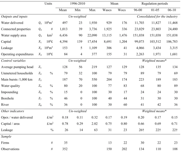
Table 1 reports the descriptive statistics for the chosen output and input variables as well as the control variables Furthermore, we include a few ratios containing relevant information: OPEX per cubic meter of water delivered, capital per square kilometer of area served, and the percentages of leakage in overall distribution input.
INSERT TABLE 1
The statistics reported in the first columns of Table 1 correspond to the whole period and are unweighted. They illustrate the high range of variation across firms, mainly due to differences in the scale of operation and population density. The two additional columns in the middle show the average for each variable by type of water distributor (WaSC/WoCs). To
18
mitigate the effect of mergers on interpreting descriptive statistics over time, the information by period reported in the last columns is either consolidated (outputs and inputs) or weighted by the volume of distributed water (control variables and other indicators). These last three columns show the values for each of the three regulatory periods discussed above.
The main facts observed on Table 1 are: 1) On the output side, we observe only a slight increase in the number of connected properties over the entire period, while aggregate water delivered volumes are relatively stable. 2) On the input side, while capital stock has increased moderately over time, operational expenditures (OPEX) have decreased dramatically. Leakage volumes also diminish but in a lower proportion, and the vast majority of this decline occurred in the regulatory period ending in 2000 (as illustrated in figure 1). 3) The control variables illustrate considerable improvements in quality, via improved drinking water quality, a decreasing number of bursts, and increasing average pumping head, which is generally associated with improved pressure provision to customers. However, while the proportion of customers receiving unmeasured water only decreased from a weighted mean of 89 percent in 1996-00 to 69 percent in the 2006-10 period, the vast majority of customers remained unmetered. 4) WoCs are significantly smaller than WaSCs with respect to all inputs and outputs dimensions. 5) Moreover, the WoCs have considerably lower leakage than the WaSCs. 6) Finally, as expected, operational cost per cubic meter of water distributed decreases while capital stock density (by square kilometer) increases, thereby further demonstrating deepening capital intensity, and OPEX reductions.
5. Results
Tables 2 to 5 contain the results of the empirical analysis. Table 2 reports a standard SFA estimation of the model, a Bayesian econometric model without leakage as an input (Model 0) and the main Bayesian results with leakage as inputs (Model 1). Given space limitations, a 90% confidence interval, the standard deviation and the results of the Geweke test are only reported for the main results. As the data has been normalized around the geometric mean, the first order coefficients can be interpreted as elasticities for the sample average firm.
The SFA and the Bayesian results are very similar; the main differences are found in the cross terms, which is the expected consequence of imposing curvature and monotonicity restrictions. The capital, leakage and OPEX elasticities for the average firm are 0.27, 0.31 and 0.42 respectively. The first order coefficients for the output variables water delivered, connected properties and supply area, imply that the average firm shows small decreasing
19
returns to scale (RTS=0.98)12. The number of connected properties is therefore the output
variable that has the most explanatory power followed by the total water delivered and the supply area (a similar order is observed for the SFA and Model 0). Since the Geweke test has a standard normal distribution, the reference value is 1.96 in absolute terms. Therefore the coefficients for capital and supply area have mild problems of convergence. All the first order coefficients are within the 90% confidence interval.
INSERT TABLE 2
Concerning the cross and squared terms, we obtain several interesting results. Output elasticities increase at increasing rate; all coefficients of the squared terms are significant and negative in Table 2. Nevertheless, their interaction counterbalances this effect. For example, keeping all things equal, increasing the amount of water delivered reduces the elasticity of connected properties (𝑎12 = 0.4072) highlighting the interaction between these two output
variables. There are three significant coefficients with respect to inputs. First as capital growths its elasticity decreases (𝑏11 = −0.1729) second, capital elasticity increases as the
supply area increases (𝑐31= 0.1005) and finally the leakage elasticity decreases if the supply
area increases (𝑐32 = −0.1271). This last result might be capturing the fact that there are less
leakage problems in low density areas. None of the interaction terms with respect to the trend are significant. Moreover, the trend, which captures technical change, is positive (technological progress) but not significant as well.
Three out of seven control variables are found to be significant. Average pumping head, the percentage of unmetered households and main bursts over 1,000 km increase input requirements. The effect of average pumping head corroborates Bottasso and Conti (2009b) findings while for the case of unmetered households, the result contradicts Saal et al. (2007). However, in Saal et al. (2007), leakage was not treated as an input. Hence, metering reduces input requirements once leakage is accounted for. The WaSC dummy was not significant, this could suggest that our overall model is otherwise sufficiently controlling for differences between the WaSCs and WoCs
INSERT TABLE 3
Table 3 reports the average input and output elasticities, the time elasticity and the shadow price of water by year and regulatory period. It also shows the average efficiency by regulatory period. We do not observe radical changes in these variables over time. Capital
20
elasticity slowly increases with time while leakage elasticity decreases which reflects the substitution of OPEX by capital previously observed in table 1. Regarding output variables, they virtually remain the same for the whole analyzed period. Time elasticity, which captures the elasticity with respect to the trend, was negative in the first two years and then continuously increasing meaning that every year there is a small technological progress (0.3% per year on average). The average efficiency increased significantly in the second regulatory period, coinciding with the period where the water prices felt in real terms following a regulatory adjustment of the price cap (Saal and Parker, 2006).
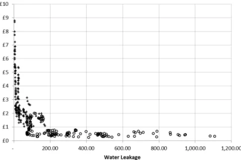
The average shadow price of water in terms of OPEX13,14 𝜙
, is about £2.01 per
cubic meter of water loss. Table 3 reveals the declining trend of the shadow price of water, as on average, it became increasingly cheaper to reduce leakage. Figures 3 shows the shadow prices of water in relation to water leakage. Notice that our results comply with the economic intuition; the operators with the higher leakage are those that value water the least15. These
figures are a persuasive argument suggesting the need to implement directed regulatory incentives in order to reduce leakage.
.
INSERT FIGURE 3
The distinction between WaSCs and WoCs reveals two interesting details (last two lines in Table 3). First, the elasticities for connected properties and OPEX for the WaSCs companies are relatively larger than for the WoCs, emphasizing the differences between these two types of water distributors. However, the most remarkable disparity comes from the shadow prices of water. For the WaSCs the average shadow price is £0.69 while for the WoCs the average price is £2.99. This large divergence is driven by the elasticities with respect to leakage and OPEX. Thus, Table 3 reveals that the average OPEX elasticities for the WaSCs(0.5422) is considerably higher than for the WoCs (0,3375) , while the opposite is true for the average leakage elasticity which is 0.3791 for the WoCs and 0.2170 for the WaSCs .
13 From now on, the shadow price of water.
14 The shadow price of water losses in terms of capital can also be computed. However, this shadow prices have
a difficult interpretation since the capital is a stock variable. In principle, it is possible to compare both shadow prices if we multiply the shadow prices of water losses in terms of capital by the weighted average cost of capital (WACC). Given the fact that the industry is very capital intensive, these shadow prices are very high (£16.83 on average.) so in practical terms, they can not play a role in curving leakage. Shadow prices of water in terms of capital are available upon request.
15 We reach to the same conclusion when we estimate the model using the SFA method without imposing any
21
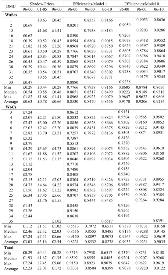
Table 4 shows the average shadow prices by regulatory period and company and the estimated efficiency scores for model 1 and 0, and also draws a distinction between WoCs and WaSCs. In total there were 35 different operators between 1995 and 2010. Although we do not identify them by name, these water supply companies share some particular features that are worth highlighting. First, the reduction of the shadow prices analyzed previously was experienced by almost all the firms in the industry. Only very few companies have estimated increases in their shadow prices for water. Corroborating our previous findings, the WaSCs show the lowest shadow prices for water. Therefore, this type of companies will have fewer difficulties in reducing leakage if the regulator decides to impose stringent rules in this regard.
In general terms, the efficiency scores remain stable across regulatory periods independently of which model was used to compute them. However, Model 1, which controls for leakage has considerably lower estimated efficiency scores, Thus for example, in the 06-10 regulatory period average estimated efficiency for all firms was 0.91122 in Model 0 and 0.8399 in Model 1 This difference could suggest that the price cap regulation system and the related cost efficiency estimates relied on by Ofwat since privatization, which have focused primarily on measuring and incentivizing cost reduction, have not properly accounted for and incentivized leakage reduction,
INSERT TABLE 4
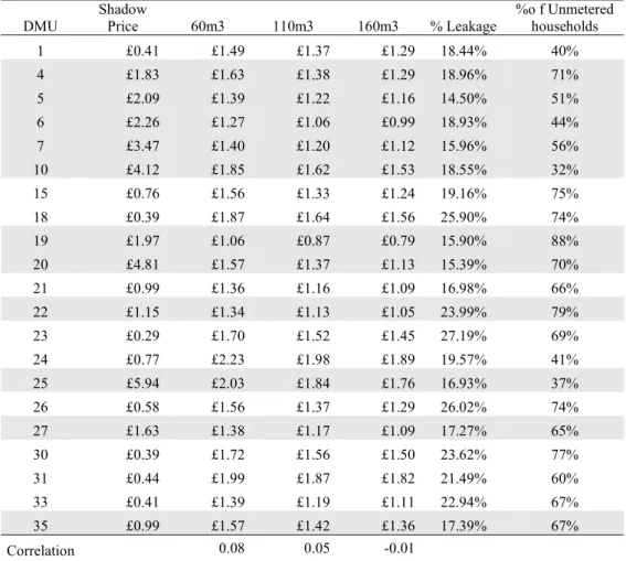
In order to understand these results by company, it is better to contextualize them by observing how much companies charge per cubic meter of water. We therefore employ data collated by Ofwat on average household water bills per cubic meter of water delivered in 2010 (Ofwat 2011). For customers who have meters, Ofwat sets out three different consumption scenarios: 60, 110 and 160m3 per year. Since our results are expressed in sterling pounds of 2010, the information is quite convenient, and we therefore relate these charges to our shadow price estimates in Table 5.
INSERT TABLE 5
Table 5 shows that WoCs do not have incentives to reduce water losses, since the price of one additional cubic meter of water sold is almost always below the estimated shadow price of water. This is in stark contrast for the WaSC ; where the estimated marginal shadow price of reducing leakage is always below the marginal benefit associated with selling an additional cubic meter of water. Paradoxically the percentage leakage for WaSCs is higher than for the WoCs (see figure 1 for the whole sector). Thus, it is not surprising that the
22
companies most affected by the mandatory targets imposed in the period 1996-2001 were the WaSCs. In contrast, the WoCs barely improved their leakage during this period, which is an outcome consistent with our finding that leakage reduction is relatively costly and hence difficult for them to achieve. Thus, our shadow price estimates strongly suggest that even though economic incentives for leakage reduction appear to exist, the WaSCs seem to be unwilling or unable to reduce their leakage levels without direct regulatory intervention. However, an alternative interpretation could be that they are responding appropriately to a regulatory system that has primarily incentivized cost reduction.
To further understand this phenomenon, it is important to keep two things in mind. Firstly, the percentage of unmetered households remained very high in 2010 (in some cases it was beyond 80%) thus a standard marginal incentive approach which assumes that one cubic meter of water saved, will be sold for additional revenue and hence profit is not relevant for most companies. This could explain the small correlation between the shadow prices and the price charged to customers; since it might be the byproduct of cross-subsidies between unmetered and metered customers. Secondly, as discussed above, WaSCs have a much higher estimated OPEX elasticity than the WoCs. Thus, a regulatory scheme that has strongly incentivized OPEX cost reductions and favored capital investments is likely to have particularly impacted their willingness to make costly efforts to reduce water leakage. Stated differently, the relevant opportunity cost might be the penalty of not achieving the regulator’s cost efficiency target, which does not account for leakage levels. Thus, in order to encourage leakage reduction, the regulatory authorities should implement policies that explicitly target this issue.
6. Conclusions
The purpose of this study is to compute the shadow price of water losses in England and Wales for the period 1995 to 2010. This information is useful to understand how much water is valued by water supply companies. Moreover, evaluation of estimated shadow prices can indicate whether the incentive regulation system that has been in place since privatization has been effective in reducing water losses. Given increasing water demand and concerns that climate change will impact water scarcity and the likelihood of severe droughts, our results have provided some important insights with regard to whether the current regulatory structure encourages good water management.
23
On average our estimates of the shadow price of water exhibit a declining trend over the period 1996 to 2010. Given moderate increases in overall water demand, coupled with an equally moderate reduction in overall water leakage, these results suggest that English and Welsh water companies have been able to reduce the marginal cost of leakage reduction. Nevertheless, given that average leakage remains at well over 20 percent, this decline in the shadow price of water also suggests that firms are not aggressively engaging in activities to reduce leakage further, as this would tend to drive the shadow price of water upward.
Moreover, our results also suggest an important distinction which must be drawn between water only companies (WoCs) and water and sewerage companies (WaSCs), as the estimated shadow price of water is markedly lower for the latter firms. In fact, the estimated shadow prices suggest that if marginal quantity pricing applied for all consumers, the WaSCs should have strong incentives to increase their profits by reducing leakage and selling the water to metered customers. However, we believe several factors help explain the fact that WaSCs do not appear to do this.
As the percentage of households with water metering is remarkably low in the U.K, the majority of households pay their water bills as a fixed amount based on the value of their property. Thus, there is a potential distortion in the water prices faced by metered customers given potential cross-subsidies between consumers with metered water and those who pay according to the valuation of their property. More significantly, the persistence of fixed cost pricing implies that it is not reasonable to assume that firms would have “normal” marginal incentives, as one cubic meter of water saved will not necessarily be sold for additional revenues. E.g., as the vast majority of water customers are not metered, the resulting absence of quantity based pricing explains why water suppliers do not seize the apparent opportunity to increase profits implied by shadow prices that are below water prices.
Thus, our results suggest that elimination of a pricing system in which customers can consume as much water as they want without paying additional fees, would significantly improve incentives to reduce water leakage. Policy makers should therefore adopt the international norm in which all customers are metered, albeit allowing for a transition period to allow consumers adjust to the new pricing regime.
In addition to considering the appropriateness of non-metered water pricing, policy makers should also consider if the post-privatization regulatory system appropriately incentivizes leakage reduction. If this system has strongly incentivized OPEX cost reductions and favored capital investments, it is also possible that it has negatively impacted incentives
24
to engage in the costly maintenance required to achieve lower leakage levels. We believe that our finding that estimated efficiency scores are substantially higher when losses are not included in our model is consistent with this conclusion. This is because it suggests that the relevant opportunity cost of leakage reducing effort might really be the penalty of not achieving the regulator’s cost efficiency targets, which similarly do not account for leakage.
A detailed consideration of an appropriate policy response to this issue is clearly beyond the scope of this paper. However, increasing water scarcity suggests that policy makers should consider how they can more appropriately incentivize regulated firms to use water resources efficiently. We might suggest the adoption of an implicit or explicit system of scarcity based water abstraction pricing by the Environment Agency. Such a system would require firms to account for not only the private costs of water supply but also environmental and scarcity costs, and would thereby improve both regulatory cost assessments and firms’ incentives to better manage scarce water resources.
In terms of the methodology, we applied O’Donnell and Coelli (2005) Bayesian framework. We estimated a translog input distance function with three outputs and three inputs which is much difficult to estimate than the 2x2 model estimated by these authors. Our model has 33 variables and it requires finding a starting point where monotonicity, homogeneity and curvature restrictions apply simultaneously. This is the main limitation of the method since it reduces significantly the possibility of testing other model specifications. For future research, it would be useful to elaborate a much more formal algorithm for finding starting points in settings with more than two input/outputs. Despite this limitation, the advantage of the Bayesian approach is that all the observation complies with the regularity conditions; which is better than relying on average information for assessing an industry.
25 7. References
Aligner DJ, Chu SF (1968) On estimating the industry production function. American Economic Review 58: 826-8S9.
BBC (2012, July). Hosepipe bans: final four companies lift restrictions, Retrieved August 28, 2012 (http://www.bbc.co.uk/news/uk-england-18764953).
Bottasso A, Conti M (2009a) Price cap regulation and the ratchet effect: a generalized index approach. Journal of Productivity Analysis 32:191-201.
Bottasso A, Conti M (2009b). Scale economies, technology and technical change in the water industry: evidence from the English water only sector. Regional Science and Urban Economics 39(2):138-147.
Bottasso A, Conti M, Piacenz M, Vannoni, D (2011) The appropriateness of the poolability assumption for multiproduct technologies: Evidence from the English water and sewerage utilities. International Journal of Production Economics 130:112-117. Chiang A (1999) Métodos Fundamentales de Economía Matemática, 3rd Ed. (F,
Muñoz-Murgui & R. Sala-Garrido Trans.) Chile: McGraw-Hill.
Coelli T, Gautier A, Perelman S, Saplacan-Pop R (2013) Estimating the cost of improving quality in electric distribution: a parametric distance function approach. Energy Policy 53:287-297.
Coelli T, Rao DSP, O'Donnell CJ, Battese GE (2005) An Introduction to Efficiency and Productivity Analysis, Springer.
Cropper M, Oates W (1992) Environmental economics, a survey. Journal of Economic Literature 30: 675-740.
Dang T, Mourougane A (2014) Estimating Shadow Prices of Pollution in Selected OECD Countries, OECD Green Growth Papers, No. 2014/02. OECD Publishing, Paris. DOI: http://dx.doi.org/10.1787/5jxvd5rnjnxs-en
Diewert WE, Wales TJ (1987) Flexible functional forms and global curvature conditions. Econometrica 55(1):44-68.
DOE. (1986) Privatisation of the Water Authorities in England and Wales, London: Department of the Environment.
Du P, Parmeter CF, Racine JS (2013) Nonparametric kernel regression with multiple predictors and multiple shape constraints. Statistica Sinica 23: 1348-1371.
Environmental Agency (2011) Environment Agency Position Statement Household Water Metering, Retrieved August 26th, 2012 (
26
Fare R, Grosskopf S, Lovell CAK, Yaisewarng S (1993) Derivation of shadow prices for undesirable outputs. The Review of Economics and Statistics 75(2): 374-380. Fare R, Grosskopf S, Noh D, Weber W (2005) Characteristics of a polluting technology:
theory and practice. Journal of Econometrics 126(2): 469-492.
Fernandez C, Osiewalski J, Steel MFJ (1997) On the use of panel data in stochastic frontier models with improper priors. Journal of Econometrics 79(1): 169-193.
Gallant R, Golub G (1984) Imposing curvature restrictions on flexible functional form. Journal of Econometrics 26: 295-321.
Garcia S, Thomas A (2001) The structure of municipal water supply costs: applications to a panel of French local communities. Journal of Productivity Analysis 16: 5-29.
Geweke J (1992) Evaluation the accuracy of sampling-based approaches to the calculation of posterior moments, in Bayesian Statistics 4, Bernardo J, Berger J, Dawid A, Smith A. (eds) Clarendon Press, Oxford, UK.
Giannikis D, Jamasb T, Pollitt M (2005) Benchmarking and incentive regulation of quality of service: an application to the UK electricity distribution networks. Energy Policy 33: 2256–2271.
Griffiths WE, O’Donnell CJ, Tan Cruz (2000) Imposing regularity conditions on a system of cost and cost-share equations: a Bayesian approach. Australian Journal of Agricultural and ResourcenEconomics 44 (1): 107–127.Growitsch C, Jamasb T, Pollitt M (2009) Quality of service, efficiency and scale in network industries: an analysis of European electricity distribution. Applied Economics 41: 20, 2555- 2570.
Henningsen A, Henning Christian (2009) Imposing regional monotonicity on translog stochastic production frontiers with a simple three-step procedure. Journal of Productivity Analysis 32:217-229.
Hosepipe bans come into force for southern and eastern England. (2012, April) The Guardian. Retrieved August 30, 2012
(
http://www.guardian.co.uk/environment/2012/apr/05/hosepipe-bans-southern-eastern-england.)
Koop G (2003) Bayesian Econometrics. Chichester, UK, John Wiley & Sons Ltd.
Koop G. Osiewalski J, Steel M (1999) The components of output growth: a stochastic frontier analysis. Oxford Bulletin of Economics and Statistics 61(4): 455-487.
Koop G. Osiewalski J, Steel M (2000) Modeling the Sources of Output Growth in a Panel of Countries. Journal of Business & Economic Statistics 18(3): 284-299.
Koop G, Steel M, Osiewalski J (1995) Posterior analysis of stochastic frontier models using Gibbs sampling. Computational Statistics 10:353-373.
27
Martins R, Coelho F, Fortunato A (2012) Water losses and hydrographical regions influence on the cost structure of the Portuguese water industry. Journal of Productivity Analysis 38:81-94.
Met Office (2012) Annual 2011, Retrieved September 6, 2012
(http://www.metoffice.gov.uk/climate/uk/2011/annual.html).
O’Donnell CJ, Coelli T (2005) A Bayesian approach to imposing curvature on distance functions. Journal of Econometrics 126: 493-523.
Office for National Statistics (2012) National Population Projections, 2010-based reference volume: Series PP2. Retrieved August 31, 2012
(
http://www.ons.gov.uk/ons/rel/npp/national-population-projections/2010-based-reference-volume--series-pp2/index.html.)
Office of Water Services (2000) Leakage and Water Efficiency.
Ofwat (2011) Your Water and Sewerage Bill 2011-12. Retrieved April, 25, 2014
(http://www.ofwat.gov.uk/consumerissues/chargesbills/prs_lft_charges2011-12.pdf)
Parmeter CF, Sun K, Henderson DJ, Kumbhakar SC (2014) Estimation and inference under economic restrictions. Journal of Productivity Analysis 41: 111-129.
Pittman R (1981) Issues in pollution control: interplant cost differences and economies of scale. Land Economics 57: 1-17.
Reinhard S, Lovell CAK, Thijssen G (1999) Econometric estimation of technical and environmental efficiency: an application to Dutch dairy farms. American Journal of Agricultural Economics 81:44-60.
Reinhard S, Lovell CAK, Thijssen G (2000) Environmental efficiency with multiple environmentally detrimental variables; estimated with SFA and DEA. European Journal of Operational Research 121:287-303.
Saal D, Parker D (2000) The Impact of Privatization and Regulation on the Water and Sewerage Industry in England and Wales: A Translog Cost Function Model. Managerial and Decision Economics 21:253-268.
Saal D, Parker D (2001) Productivity and Price Performance in the Privatized Water and Sewerage Companies in England and Wales. Journal of Regulatory Economics 20:61-90.
Saal D, Parker D (2006) Assessing the Performance of Water Operations in the English and Welsh Water Industry: A Lesson in the Implications of Inappropriately Assuming a Common Frontier. Performance Measurement and Regulation of Network Industries, Coelli, T. & Lawrence, D. (eds) Edward Elgar.
Saal D, Parker D, Weyman-Jones T (2007) Determining the contribution of technical change, efficiency change and scale change to productivity growth in the privatized English
28
and Welsh water and sewerage industry: 1985–2000. Journal of Productivity Analysis 28: 127-139.
Shy O (2001) The Economics of Network Industries. Cambridge University Press, Cambridge.
Simon C, Blume L (1994) Mathematics for Economists, New York, W.W. Norton & Company Inc.
Terrell D (1996) Incorporating monotonicity and concavity conditions in flexible functional forms. Journal of Applied Econometrics 11(2) 179-194.
Torres M, Morrison Paul CJ (2006) Driving forces for consolidation or fragmentation of the US water utility industry: a cost function approach with endogenous output. Journal of Urban Economics 59(1), 104-120.
Van Soest D, List, J, Jeppesen T (2006) Shadow prices, environmental stringency, and international competitiveness. European Economic Review 50:1151-1167. Wolff H, Heckelei T, Mittelhammer R (2010) Imposing curvature and monotonicity on
flexible functional forms: an efficient regional approach. Computational Economics 36(4): 309-339.
Yaisawarng S, Klein D (1994) The effects of sulfur dioxin controls on productivity change in the U.S. electric power industry. The Review of Economics and Statistics 447-460. Yu W, Jamasb T, Pollitt M (2008) Does weather explain the cost and quality? An analysis of
UK electricity distribution companies. Electricity Policy Research Group Working Papers, No.EPRG0827. Cambridge: University of Cambridge.
29
30