Constructive Nonlinear Control

(1)

Preface

In this book several streams of nonlinear control theory are merged and di-rected towards a constructive solution of the feedback stabilization problem. Analytic, geometric and asymptotic concepts are assembled as design tools for a wide variety of nonlinear phenomena and structures. Differential-geometric concepts reveal important structural properties of nonlinear systems, but al-low no margin for modeling errors. To overcome this deficiency, we combine them with analytic concepts of passivity, optimality and Lyapunov stability. In this way geometry serves as a guide for construction of design procedures, while analysis provides robustness tools which geometry lacks.

Our main tool is passivity. As a common thread, it connects all the chapters of the book. Passivity properties are induced by feedback passivation designs. Until recently, these designs were restricted to weakly minimum phase systems with relative degree one. Our recursive designs remove these restrictions. They are applicable to wider classes of nonlinear systems characterized by feedback, feedforward, and interlaced structures.

After the introductory chapter, the presentation is organized in two major parts. The basic nonlinear system concepts - passivity, optimality, and stabil-ity margins - are presented in Chapters 2 and 3 in a novel way as design tools. Most of the new results appear in Chapters 4, 5, and 6. For cascade systems, and then, recursively, for larger classes of nonlinear systems, we construct de-sign procedures which result in feedback systems with optimality properties and stability margins.

The book differs from other books on nonlinear control. It is more design-oriented than the differential-geometric texts by Isidori [43] and Nijmeijer and Van der Schaft [84]. It complements the books by Krstić, Kanellakopoulos and Kokotović [61] and Freeman and Kokotović [26], by broadening the class of systems and design tools. The book is written for an audience of graduate students, control engineers, and applied mathematicians interested in control theory. It is self-contained and accessible with a basic knowledge of control theory as in Anderson and Moore [1], and nonlinear systems as in Khalil [56].

(2)

For clarity, most of the concepts are introduced through and explained by examples. Design applications are illustrated on several physical models of practical interest.

The book can be used for a first level graduate course on nonlinear control, or as a collateral reading for a broader control theory course. Chapters 2, 3, and 4 are suitable for a first course on nonlinear control, while Chapters 5 and 6 can be incorporated in a more advanced course on nonlinear feedback design.

∗ ∗ ∗

The book is a result of the postdoctoral research by the first two authors with the third author at the Center for Control Engineering and Computation, University of California, Santa Barbara. In the cooperative atmosphere of the Center, we have been inspired by, and received help from, many of our colleagues. The strongest influence on the content of the book came from Randy Freeman and his ideas on inverse optimality. We are also thankful to Dirk Aeyels, Mohammed Dahleh, Miroslav Krsti´c, Zigang Pan, Laurent Praly and Andrew Teel who helped us with criticism and advice on specific sections of the book. Gang Tao generously helped us with the final preparation of the manuscript. Equally generous were our graduate students Dan Fontaine with expert execution of figures, Srinivasa Salapaka and Michael Larsen with simulations, and Kenan Ezal with proofreading.

Our families contributed to this project by their support and endurance. Ivana, Edith, Simon and Filip often saw their fathers absent or absent-minded. Our wives, Natalie, Seka, and Anna unwaveringly carried the heaviest burden. We thank them for their infinite stability margins.

∗ ∗ ∗

The support for research that led to this book came from several sources. Ford Motor Company supported us financially and encouraged one of its re-searchers (MJ) to continue this project. Support was also received form BAEF and FNRS, Belgium (RS). The main support for this research program (PK) are the grants NSF ECS-9203491 and AFOSR F49620-95-1-0409.

Rodolphe Sepulchre Mrdjan Jankovi´c Petar Kokotovi´c Santa Barabra, California, August 1996

(3)

Chapter 1 Introduction

Control theory has been extremely successful in dealing with linear time-invariant models of dynamic systems. A blend of state space and frequency domain methods has reached a level at which feedback control design is system-atic, not only with disturbance-free models, but also in the presence of distur-bances and modeling errors. There is an abundance of design methodologies for linear models: root locus, Bode plots, LQR-optimal control, eigenstruc-ture assignment, H-infinity, µ-synthesis, linear matrix inequalities, etc. Each of these methods can be used to achieve stabilization, tracking, disturbance attenuation and similar design objectives.

The situation is radically different for nonlinear models. Although several nonlinear methodologies are beginning to emerge, none of them taken alone is sufficient for a satisfactory feedback design. A question can be raised whether a single design methodology can encompass all nonlinear models of practical interest, and whether the goal of developing such a methodology should even be pursued. The large diversity of nonlinear phenomena suggests that, with a single design approach most of the results would end up being unnecessarily conservative. To deal with diverse nonlinear phenomena we need a comparable diversity of design tools and procedures. Their construction is the main topic of this book.

Once the “tools and procedures” attitude is adopted, an immediate task is to determine the areas of applicability of the available tools, and critically evaluate their advantages and limitations. With an arsenal of tools one is encouraged to construct design procedures which exploit structural proper-ties to avoid conservativeness. Geometric and analytic concepts reveal these properties and are the key ingredients of every design procedure in this book. Analysis is suitable for the study of stability and robustness, but it often disregards structure. On the other hand, geometric methods are helpful in

(10)

determining structural properties, such as relative degree and zero dynamics, but, taken alone, do not guarantee stability margins, which are among the prerequisites for robustness. In the procedures developed in this book, the ge-ometry makes the analysis constructive, while the analysis makes the gege-ometry more robust.

Chapters 2 and 3 present the main geometric and analytic tools needed for the design procedures in Chapters 4, 5, and 6. Design procedures in Chapter 4 are constructed for several types of cascades, and also serve as building blocks in the construction of recursive procedures in Chapters 5 and 6.

The main recursive procedures are backstepping and forwarding. While backstepping is known from [61], forwarding is a procedure recently developed by the authors [46, 95]. This is its first appearance in a book. An important feature of this procedure is that it endows the systems with certain optimality properties and desirable stability margins.

In this chapter we give a brief preview of the main topics discussed in this book.

1.1 Passivity, Optimality, and Stability

1.1.1 From absolute stability to passivity

Modern theory of feedback systems was formed some 50-60 years ago from two separate traditions. The Nyquist-Bode frequency domain methods, developed for the needs of feedback amplifiers, became a tool for servomechanism design during the Second World War. In this tradition, feedback control was an outgrowth of linear network theory and was readily applicable only to linear time-invariant models.

The second tradition is more classical and goes back to Poincar´e and Lya-punov. This tradition, subsequently named the state-space approach, employs the tools of nonlinear mechanics, and addresses both linear and nonlinear mod-els. The main design task is to achieve stability in the sense of Lyapunov of feedback loops which contain significant nonlinearities, especially in the ac-tuators. A seminal development in this direction was the absolute stability problem of Lurie [70].

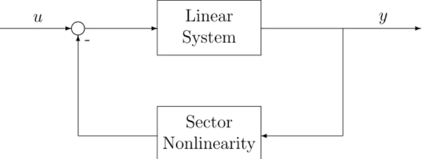
In its simplest form, the absolute stability problem deals with a feedback loop consisting of a linear block in the forward path and a nonlinearity in the feedback path, Figure 1.1. The nonlinearity is specified only to the extent that it belongs to a “sector”, or, in the multivariable case, to a “cone”. In other words, the admissible nonlinearities are linearly bounded. One of the absolute

(11)

- - Linear System -Sector Nonlinearity¾ 6 u -y

Figure 1.1: The absolute stability problem.

stability results is a Lyapunov function construction for this class of systems. The stability property is “absolute” in the sense that it is preserved for any nonlinearity in the sector. Hence, a “sector stability margin” is guaranteed.

During a period of several years, the frequency domain methods and the ab-solute stability analysis coexisted as two separate disciplines. Breakthroughs by Popov in the late 1950’s and early 1960’s dramatically changed the land-scape of control theory. While Popov’s stability criterion [87] was of major importance, even more important was his introduction of the concept of pas-sivity as one of the fundamental feedback properties [88].

Until the work of Popov, passivity was a network theory concept dealing with rational transfer functions which can be realized with passive resistances, capacitances and inductances. Such transfer functions are restricted to have relative degree (excess of the number of poles over the number of zeros) not larger than one. They are called positive real because their real parts are positive for all frequencies, that is, their phase lags are always less than 90 degrees. A key feedback stability result from the 1960’s, which linked passivity with the existence of a quadratic Lyapunov function for a linear system, is the celebrated Kalman-Yakubovich-Popov (KYP) lemma also called Positive Real Lemma. It has spawned many significant extensions to nonlinear systems and adaptive control.

1.1.2 Passivity as a phase characteristic

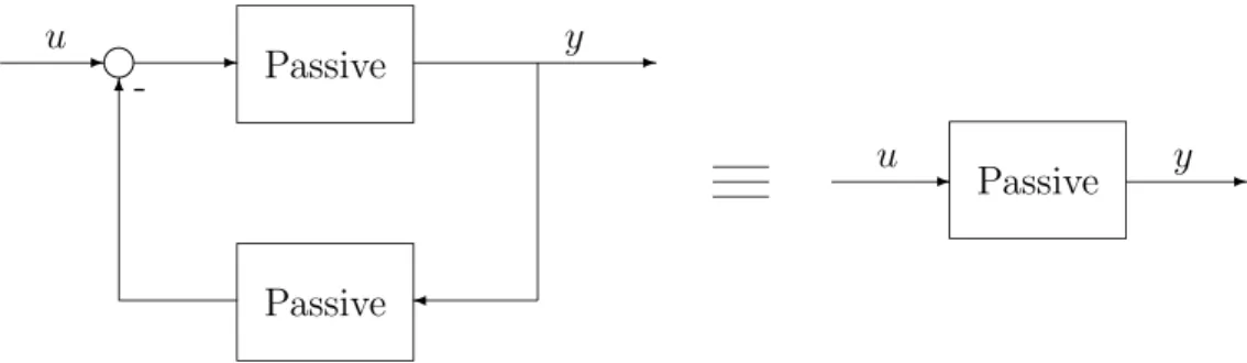
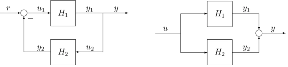
The most important passivity result, and also one of the fundamental laws of feedback, states that a negative feedback loop consisting of two passive systems is passive. This is illustrated in Figure 1.2. Under an additional detectability condition this feedback loop is also stable.

(12)

- -6 Passive Passive -¾ - _Passive -u y u y

Figure 1.2: The fundamental passivity result.

passive blocks in the feedback connection of Figure 1.2 are linear. Then their transfer functions are positive real, that is, with the phase lag not larger than 90 degrees. Hence, the phase lag over the entire feedback loop is not larger than 180 degrees. By the Nyquist-Bode criterion, such a linear feedback loop is stable for all feedback gains, that is, it possesses an “infinite gain margin”. When the two blocks in the feedback loop are nonlinear, the concept of pas-sivity can be seen to extend the Nyquist-Bode 180 degree phase lag criterion to nonlinear systems. For nonlinear systems, passivity can be therefore inter-preted as a “phase” property, a complement of the gain property characterized by various small gain theorems such as those presented in [18].

In the early 1970’s, Willems [120] systematized passivity (and dissipativity) concepts by introducing the notions of storage function S(x) and supply rate w(u, y), where x is the system state, u is the input, and y is the output. A system is passive if it has a positive semidefinite storage function S(x) and a bilinear supply rate w(u, y) = uT_{y, satisfying the inequality}

S(x(T ))_{− S(x(0)) ≤}

Z T

0 w(u(t), y(t)) dt (1.1.1)

for all u and T ≥ 0. Passivity, therefore, is the property that the increase in storage S is not larger than the integral amount supplied. Restated in the derivative form

˙

S(x) _{≤ w(u, y)} (1.1.2)

passivity is the property that the rate of increase of storage is not higher than the supply rate. In other words, any storage increase in a passive system is due solely to external sources. The relationship between passivity and Lyapunov stability can be established by employing the storage S(x) as a Lyapunov function. We will make a constructive use of this relationship.

(13)

1.1.3 Optimal control and stability margins

Another major development in the 1950’s and 1960’s was the birth of op-timal control twins: Dynamic Programming and Maximum Principle. An optimality result crucial for feedback control was the solution of the optimal linear-quadratic regulator (LQR) problem by Kalman [50] for linear systems ˙x = Ax+Bu. The well known optimal control law has the form u =_{− B}T _{P x,}

where x is the state, u is the control and P is the symmetric positive definite solution of a matrix algebraic Riccati equation. The matrix P determines the optimal value xT _{P x of the cost functional, which, at the same time, is a}

Lya-punov function establishing the asymptotic stability of the optimal feedback system.

A remarkable connection between optimality and passivity, established by Kalman [52], is that a linear system can be optimal only if it has a passivity property with respect to the output y = BT_{P x. Furthermore, optimal linear}

systems have infinite gain margin and phase margin of 60 degrees.

These optimality, passivity, and stability margin properties have been ex-tended to nonlinear systems which are affine in control:

˙x = f (x) + g(x)u (1.1.3)

A feedback control law u = k(x) which minimizes the cost functional J =

Z _∞

0 (l(x) + u

2_)dt _(1.1.4)

where l(x) is positive semidefinite and u is a scalar, is obtained by minimizing the Hamiltonian function

H(x, u) = l(x) + u2+ ∂V

∂x(f (x) + g(x)u) (1.1.5)

If a differentiable optimal value function V (x) exists, then the optimal control law is in the “LgV -form”:

u = k(x) =₋1 2LgV (x) =− 1 2 ∂V ∂xg(x) (1.1.6)

The optimal value function V (x) also serves as a Lyapunov function which, along with a detectability property, guarantees the asymptotic stability of the optimal feedback system. The connection with passivity was established by Moylan [80] by showing that, as in the linear case, the optimal system has an infinite gain margin thanks to its passivity property with respect to the output y = LgV .

(14)

In Chapters 2 and 3 we study in detail the design tools of passivity and optimality, and their ability to provide desirable stability margins. A particu-lar case of interest is when V (x) is a Lyapunov function for ˙x = f (x), which is stable but not asymptotically stable. In this case, the control law u =−LgV

adds additional “damping”. This damping control is again in the “LgV -form”.

It is often referred to as “Jurdjevic-Quinn feedback” [49] and will frequently appear in this book.

What this book does not include are methods applicable only to linearly bounded nonlinearities. Such methods, including various small gain theorems [18], H-infinity designs with bounded uncertainties [21], and linear matrix in-equality algorithms [7] are still too restrictive for the nonlinear systems consid-ered in this book. Progress has been made in formulating nonlinear small gain theorems by Mareels and Hill [71], Jiang, Teel and Praly [48], among others, and in using them for design [111]. Underlying to these efforts, and to several results of this book, is the concept of input-to-state stability (ISS) of Son-tag [103] and its relationship to dissipativity. The absolute stability tradition has also continued with a promising development by Megretski and Rantzer [76], where the static linear constraints are replaced by integral quadratic con-straints.

1.2 Feedback Passivation

1.2.1 Limitations of feedback linearization

Exciting events in nonlinear control theory of the 1980’s marked a rapid devel-opment of differential-geometric methods which led to the discovery of several structural properties of nonlinear systems. The interest in geometric methods was sparked in the late 70’s by “feedback linearization,” in which a nonlinear system is completely or partially transformed into a linear system by a state diffeomorphism and a feedback transformation.

However, feedback linearization may result not only in wasteful controls, but also in nonrobust systems. Feedback linearizing control laws often destroy inherently stabilizing nonlinearities and replace them with destabilizing terms. Such feedback systems are without any stability margins, because even the smallest modeling errors may cause a loss of stability.

A complete or partial feedback linearization is performed in two steps. First, a change of coordinates (diffeomorphism) is found in which the system appears “the least nonlinear.” This step is harmless. In the second step, a

(15)

control is designed to cancel all the nonlinearities and render the system linear. This step can be harmful because it often replaces a stabilizing nonlinearity by its wasteful and dangerous negative.

Fortunately, the harmful second step of feedback linearization is avoid-able. For example, a control law minimizing a cost functional like (1.1.4) does not cancel useful nonlinearities. On the contrary, it employs them, espe-cially for large values of x which are penalized more. This motivated Freeman and Kokotovi´c [25] to introduce an “inverse optimal” design in which they replace feedback linearization by robust backstepping and achieve a form of worst-case optimality. Because of backstepping, this design is restricted to a lower-triangular structure with respect to nonlinearities which grow faster than linear. A similar idea of employing optimality to avoid wasteful cancel-lations is pursued in this book, but in a different setting and for a larger class of systems, including the systems that cannot be linearized by feedback.

1.2.2 Feedback passivation and forwarding

Lyapunov designs in this book achieve stability margins by exploiting the connections of stability, optimality and passivity. Geometric tools are used to characterize the system structure and to construct Lyapunov functions.

Most of the design procedures in this book are based on feedback passiva-tion. For the partially linear cascade, including the Byrnes-Isidori normal form [13], the problem of achieving passivity by feedback was first posed and solved by Kokotovi´c and Sussmann [59]. A general solution to the feedback passi-vation problem was given by Byrnes, Isidori and Willems [15] and is further refined in this book.

Because of the pursuit of feedback passivation, the geometric properties of primary interest are the relative degree of the system and the stability of its zero dynamics. The concepts of relative degree and zero dynamics, along with other geometric tools are reviewed in Appendix A. A comprehensive treatment of these concepts can be found in the books by Isidori [43], Nijmeijer and van der Schaft [84], and Marino and Tomei [73].

Achieving passivity with feedback is an appealing concept. However, in the construction of feedback passivation designs which guarantee stability margins, there are two major challenges. The first challenge is to avoid nonrobust cancellations. In this book this is achieved by rendering the passivating control optimal with respect to a cost functional (1.1.4). It is intuitive that highly penalized control effort will not be wasted to cancel useful nonlinearities, as confirmed by the stability margins of optimal systems in Chapter 3.

(16)

The second challenge of feedback passivation is to make it constructive. This is difficult because, to establish passivity, which is an input-output con-cept, we must select an output y and construct a positive semidefinite storage function S(x) for the supply rate uT_{y. In the state feedback stabilization the}

search for an output is a part of the design procedure. This search is guided by the structural properties: in a passive system the relative degree must not be larger than one and the zero dynamics must not be unstable (“nonmini-mum phase”). Like in the linear case, the nonlinear relative degree and the nonlinear dynamics subsystem are invariant under feedback. If the zero-dynamics subsystem is unstable, the entire system cannot be made passive by feedback. For feedback passivation one must search for an output with respect to which the system will not only have relative degree zero or one, but also be “weakly minimum phase” (a concept introduced in [92] to include some cases in which the zero-dynamics subsystem is only stable, rather than asymptotically stable).

Once an output has been selected, a positive semidefinite storage function S(x) must be found for the supply rate uT_{y. For our purpose this storage}

function serves as a Lyapunov function. It is also required to be the optimal value of a cost functional which penalizes the control effort.

One of the perennial criticisms of Lyapunov stability theory is that it is not constructive. Design procedures developed in this book remove this deffi-ciency for classes of systems with special structures. Backstepping solves the stabilization problem for systems having a lower-triangular structure, while forwarding does the same for systems with an upper-triangular structure. This methodology, developed by the authors [46, 95], evolved from an earlier nested saturation design by Teel [109] and recent results by Mazenc and Praly [75].

1.3 Cascade Designs

1.3.1 Passivation with composite Lyapunov functions

The design procedures in this book are first developed for cascade systems. The cascade is “partially linear” if one of the two subsystems is linear, that is

˙z = f (z) + ψ(z, ξ), ψ(z, 0) = 0

˙ξ = Aξ + Bu (1.3.1)

where (A, B) is a stabilizable pair. Even when the subsystem ˙z = f (z) is GAS, it is the interconnection term ψ(z, ξ) which determines whether the entire cascade is stabilizable or not.

(17)

Applying the result that a feedback connection of two passive systems is passive, the cascade (1.3.1) can be rendered passive if it can be represented as a feedback interconnection of two passive systems. To this end, an output y1 = h1(ξ) = Cξ is obtained for the ξ-subsystem by a factorization of the

interconnection term:

ψ(z, ξ) = ˜ψ(z, ξ)h1(ξ) (1.3.2)

The output y1 of the ξ-subsystem is the input of the z-subsystem. We let W (z)

be the z-subsystem Lyapunov function such that LfW (z) ≤ 0. Then for the

input h1(ξ), the z-subsystem is passive with respect to the output y2 = L_ψ˜W

and W (z) is its storage function. It is now sufficient that the ξ-subsystem with the output y1 = h1(ξ) = Cξ can be made passive by a feedback transformation

u = Kx + Gv. Then a composite Lyapunov function for the whole cascade is V (z, ξ) = W (z)+ξT_{P ξ, where P > 0 satisfies the Positive Real Lemma for the}

(A + BK, BG, BT_{P ). Such a matrix P exists if the linear subsystem (A, B, C)}

is feedback passive. Because the relative degree and the zero dynamics are invariant under feedback, a structural restriction on (A,B,C) is to be relative degree one and weakly minimum phase.

A similar construction of a composite Lyapunov function

V (z, ξ) = W (z) + U (ξ) (1.3.3)

is possible when both subsystems in the cascade are nonlinear ˙z = f (z) + ˜ψ(z, ξ)h1(ξ)

˙ξ = a(ξ, u) (1.3.4)

and when the assumption on ˙z = f (z) is relaxed to be only GS (globally stable), with a Lyapunov function W (z) such that LfW (z) ≤ 0. Again, the

z-subsystem is passive with the input-output pair u2 = h1(ξ) and y2 = L_ψ˜W .

The entire cascade is rendered passive if the ξ-subsystem with output y1 =

h1(ξ) is made passive by feedback. As in the linear case, the relative degree

and zero-dynamics restrictions must be satisfied and a storage function U (ξ) must be found.

In Chapter 4 several versions of such passivation designs are employed to stabilize translational oscillations of a platform using a rotating actuator.

1.3.2 A structural obstacle: peaking

One of the novelties of this book is the treatment in Chapter 4 of an often overlooked obstacle to global and semiglobal stabilization – the peaking phe-nomenon. In its simplest form this phenomenon occurs in the linear system

(18)

˙ξ = Aξ + Bu when the gain K in the state feedback u = Kξ is chosen to place the eigenvalues of A + BK to the left of Re{s} = −a < 0. For a fast convergence of ξ to zero, the value of a must be large, that is, the gain K must be high.

Each state component ξi is bounded by γie−at where γi depends not only

on the initial condition ξ(0), but also on the rate of decay a, that is γi = ˜γiaπi.

The peaking states are those ξi’s for which the peaking exponent πi is one or

larger, while for the nonpeaking states this exponent is zero. In a partially linear cascade (1.3.1), an undesirable effect of peaking in the linear subsystem is that it limits the size of the achievable stability region, as we now illustrate. In the cascade

˙z =_{−z + yz}2

˙ξ1 = ξ2

˙ξ2 = u, y = c1ξ1+ c2ξ2

(1.3.5) the z-equation can be solved explicitly:

z(t) = e−tz(0)[1− z(0)

Z t 0 e

−τ_{y(τ ) dτ ]}−1

Clearly, to avoid the escape of z(t) to infinity in finite time, it is necessary that the following bound be satisfied

z(0)

Z _∞

0 e

−t_{y(t) dt}_{≤ 1} _(1.3.6)

With partial-state feedback u = k1ξ1+ k2ξ2 the decay of y(t) is exponential,

|y(t)| ≤ γe−at_{, and the bound (1.3.6) is satisfied if}

z(0)γ

a + 1 ≤ 1 (1.3.7)

If y(t) is not peaking, that is if γ does not grow with a, then z(0) can be allowed to be as large as desired by making a sufficiently large. Thus, when y is a nonpeaking output of the linear subsystem, that is, when y can be forced to decay arbitrarily fast without peaking, then the entire cascade can be semiglobally stabilized.

Even when y is a nonpeaking output, not every feedback law will achieve fast decay of y without peaking, as we illustrate with the “high-gain” design

u =−a2_ξ

1− 2aξ2 (1.3.8)

for ξ-subsystem in (1.3.5). This high-gain control law places the eigenvalues at λ1 = λ2 =−a. A simple calculation shows that in this case ξ1 is a nonpeaking

(19)

state, while ξ2 is peaking with π2 = 1. Thus, y = ξ1 satisfies (1.3.7) and the

semiglobal stability is achieved. On the other hand, when y = ξ2 the bound

(1.3.6) for (ξ1(0), ξ2(0)) = (1, 0) is

z(0)a2

a2_{+ 1} ≤ 1

and semiglobal stability cannot be achieved: no increase of a will allow z(0) to be larger than one.

To see that y = ξ2 is in fact a nonpeaking output we now use the “two

time-scale” design

u =_{−ξ − (a +} 1

a)ξ2 (1.3.9)

which, for large a, renders λ2 = −a “fast”, and λ1 = −1_a “slow.” A simple

calculation shows that, with feedback (1.3.9), the output y = ξ2 still has the

fast decay rate a, but is nonpeaking, that is, it satisfies the bound (1.3.7) which guarantees semiglobal stability.

We have thus demonstrated that with either y = ξ1 (or y = ξ2) semiglobal

stabilization of the cascade (1.3.5) is possible with partial-state feedback de-sign (1.3.8) (or (1.3.9)), each rendering the decay of y arbitrarily fast without peaking.

Can global stabilization also be achieved? The answer is affirmative, but for this we must use full-state feedback u(ξ1, ξ2, z). For y = ξ2 we can design

such a feedback law using passivation discussed in the preceding section, while for y = ξ1, we can use a backstepping design, to be discussed later. These

two full-state feedback designs satisfy the bound (1.3.6) for all z(0) by forcing y(t) to depend on z(t) and to contribute to the stabilization process via the interconnection term yz2_.

In the discussion thus far we have mentioned the control laws which avoid output peaking for y = ξ1and y = ξ2 in (1.3.5). However, it can be shown that

output peaking cannot be avoided if y = ξ1− ξ2. In this case, neither global

nor semiglobal stabilization of the cascade (1.3.5) is possible. With y = ξ1− ξ2

the double integrator is “strictly” nonminimum phase and all such systems are peaking systems.

For the cascade (1.3.1), with ˙z = f (z) being GAS, the peaking phenomenon and the structure of the interconnection term ψ(z, ξ) determine whether global or semiglobal stabilization is possible. If the interconnection term ψ(z, ξ) contains peaking states multiplied with functions of z which grow faster than linear, global stabilization may be impossible. To determine whether this is the case, the interconnection is factored as ˜ψ(z, ξ0)Cξ, where Cξ is treated

(20)

as the output of the linear subsystem and ξ0 denotes the nonpeaking states.

Now the problem is to stabilize the linear subsystem while preventing the peaking in the output Cξ. The class of output nonpeaking linear systems is characterized in Chapter 4 where it is shown that strictly nonminimum phase linear systems are peaking systems. Our new analysis encompasses both fast and slow peaking.

We reiterate that peaking is an obstacle not only to global stabilization, but also to more practical semiglobal stabilization which is defined as the possibility to guarantee any prespecified bounded stability region. Our analysis of peaking in Chapter 4 applies and extends earlier results by Mita [79], Francis and Glover [20], and the more recent results by Sussmann and Kokotovi´c [105], and Lin and Saberi [67].

1.4 Lyapunov Constructions

1.4.1 Construction of the cross-term

The most important part of our design procedures is the construction of a Lyapunov function for an uncontrolled subsystem. In Chapter 5 this task is addressed with a structure-specific approach and a novel Lyapunov construc-tion is presented for the cascade

(Σ0)

(

˙z = f (z) + ψ(z, ξ)

˙ξ = a(ξ) (1.4.1)

where ˙z = f (z) is globally stable and ˙ξ = a(ξ) is globally asymptotically stable and locally exponentially stable. Such constructions have not appeared in the literature until the recent work by Mazenc and Praly [75] and the authors [46]. Chapter 5 presents a comprehensive treatment of several exact and approximate Lyapunov constructions.

The main difficulty in constructing a Lyapunov function for (Σ0) is due to

the fact that ˙z = f (z) is only globally stable, rather than globally asymptoti-cally stable, so that simple composite Lyapunov functions such as W (z)+U (ξ) in (1.3.3) are not suitable.

Our main construction is aimed at finding the cross-term Ψ(z, ξ) for a more general Lyapunov function

V0(z, ξ) = W (z) + Ψ(z, ξ) + U (ξ)

where W (z) and U (ξ) are the Lyapunov functions of the subsystems. The cross-term Ψ(z, ξ) is needed to achieve nonpositivity of

˙

(21)

Because LψW is indefinite, ˙Ψ is constructed to eliminate it, that is ˙Ψ =

−LψW . In Chapter 5 we prove the existence and continuity of Ψ(z, ξ) under

the conditions

k∂W

∂z k kzk ≤ cW (z), as kzk → ∞ (1.4.2)

kψ(z, ξ)k ≤ γ1(kξk)kzk + γ2(kξk) (1.4.3)

The first condition restricts the growth of W to be polynomial. The second condition restricts the growth of the interconnection term ψ(z, ξ) to be linear in _{kzk. These conditions are structural and cannot be removed without} ad-ditional restrictions on f (z) and ψ(z, ξ). An expression for Ψ(z, ξ), which for special classes of cascades can be obtained explicitly, is the line integral

Ψ(z, ξ) =

Z _∞

0 LψW (˜z(s; (z, ξ)), ˜ξ(s, ξ))ds (1.4.4)

along the solution of (Σ0) which starts at (z, ξ). In general, this integral

is either precomputed, or implemented with on-line numerical integrations. Approximate evaluations of Ψ(z, ξ) from a PDE can also be employed.

1.4.2 A benchmark example

As an illustration of the explicit construction of the cross-term Ψ(z, ξ) and its use in a passivation design we consider the system

˙x1 = x2+ θx23

˙x2 = x3

˙x3 = ˜u

(1.4.5) We first let θ = 1 and later allow θ to be an unknown constant parameter. This system cannot be completely linearized by a change of coordinates and feedback. For y = x2+ x3 it has the relative degree one and can be written as

˙x1 = x2+ x22+ (2x2+ y)y

˙x2 = −x2+ y

˙y = −y + u

(1.4.6) where we have set ˜u =−2y + x2+ u. To proceed with a passivation design we

observe that the zero-dynamics subsystem ˙x1 = x2+ x22

˙x2 = −x2

is stable, but not asymptotically stable. For this subsystem we need a Lya-punov function and, to construct it, we consider x1 as z, x2 as ξ and view

(22)

the zero-dynamics subsystem as the cascade system (Σ0). For W = x21 the

line-integral (1.4.4) yields the explicit expression Ψ(x1, x2) = (x1+ x2+ x2 2 2) 2 − x21

which, along with U (x2) = x22, results in the Lyapunov function

V0(x1, x2) = (x1+ x2+ x2 2 2) 2_{+ x}2 2

Returning to the normal form (1.4.6) we get the cascade (1.3.1), in the notation (z1, z2, ξ) instead of (x1, x2, y). The interconnection term ψT = [2x2+y, 1]Ty is

already factored because y = ξ and the ξ-subsystem is passive with the storage function S(y) = y2_{. Applying the passivation design from Section 1.3.1, where}

V0(x1, x2) plays the role of W (z) and ˜ψT = [2x2+ y, 1]T, the resulting feedback

control is u =−∂V0 ∂x1 (2x2+ y)− ∂V0 ∂x2

Using V = V0(x1, x2) + y2 as a Lyapunov function it can be verified that the

designed feedback system is globally asymptotically stable. It is instructive to observe that this design exploits two nested cascade structures: first, the zero-dynamics subsystem is itself a cascade; and second, it is also the nonlinear part of the overall cascade (1.4.6).

An alternative approach, leading to recursive forwarding designs in Chapter 6, is to view the same system (1.4.5) as the cascade of the double integrator ˙x2 = x3, ˙x3 = ˜u with the x1-subsystem. The double integrator part is first

made globally exponentially stable by feedback, say u =−x2− 2x3 + v. It is

easy to verify that with this feedback the whole system is globally stable. To proceed with the design, a Lyapunov function V (x) is to be constructed for the whole system such that, with respect to the passivating output y = _∂x∂V₃, the system satisfies a detectability condition. The global asymptotic stability of the whole system can then be achieved with the damping control v =−∂V

∂x3.

Again, the key step is the construction of the cross-term Ψ for the Lyapunov function V (x). In this case the cross-term is

Ψ(x1, x2, x3) = 1 2(x1+ 2x2 + x3+ 1 2(x 2 2+ x23)2)2− 1 2x 2 1 and results in V (x) = 1 2(x1+ 2x2+ x3+ 1 2(x 2 2 + x23)2)2+ 1 2x 2 2+ 1 2x 2 3

(23)

1.4.3 Adaptive control

While adaptive control is not a major topic of this book, the Lyapunov con-struction in Chapter 5 is extended to nonlinear systems with unknown constant parameters, such as the system (1.4.5) with unknown θ. Without a known bound on θ, the global stabilization problem for this benchmark system has not been solved before. Its solution can now be obtained by constructing the same control law as if θ were known. Then the unknown parameter is replaced by its estimate, and the Lyapunov function is augmented by a term penalizing the parameter estimation error. Finally, a parameter update law is designed to make the time-derivative of the augmented Lyapunov function negative. This step, in general, requires that the estimates be overparameterized. Thus, for the above example, instead of one, estimates of two parameters are needed. This adaptive design is presented in Chapter 5.

1.5 Recursive Designs

1.5.1 Obstacles to passivation

With all its advantages, feedback passivation has not yet become a widely used design methodology. Many passivation attempts have been frustrated by the requirements that the system must have a relative degree one and be weakly minimum phase. As the dimension of the system increases, searching for an output which satisfies these requirements rapidly becomes an unwieldy task. Even for a highly structured system such as

˙z = f (z) + ˜ψ(z, ξi)ξi, i∈ {1, . . . , n} ˙ξ1 = ξ2 ˙ξ2 = ξ3 ... ˙ξn = u, (1.5.1)

with globally asymptotically stable ˙z = f (z), feedback passivation is difficult because each candidate output y = ξi fails to satisfy at least one of the two

passivity requirements. Thus, if y = ξ1, the system is minimum phase, but it

has a relative degree n. On the other hand, if y = ξn, the relative degree is

one, but the system is not weakly minimum phase because the zero-dynamics subsystem contains an unstable chain of integrators. For all other choices y = ξi, neither the relative degree one, nor the weak minimum phase requirement

(24)

The recursive step-by-step constructions in Chapter 6 circumvent the struc-tural obstacles to passivation. At each step, only a subsystem is considered, for which the feedback passivation is feasible. Each of the two recursive proce-dures, backstepping and forwarding, removes one of the obstacles to feedback passivation.

1.5.2 Removing the relative degree obstacle

Backstepping removes the relative degree one restriction. This is illustrated with the cascade (1.5.1) with i = 1, that is with y = ξ1. With this output, the

relative degree one requirement is not satisfied for the entire system. To avoid this difficulty, the backstepping procedure first isolates the subsystem

˙z = f (z) + ˜ψ(z, ξ1)ξ1,

˙ξ1 = u1,

y1 = ξ1

(1.5.2)

With u1 as the input, this system has relative degree one and is weakly

min-imum phase. Therefore, we can construct a Lyapunov function V1(z, ξ1) and

a stabilizing feedback u1 = α1(z, ξ1). In the second step, this subsystem is

augmented by the ξ2-integrator:

˙z = f (z) + ˜ψ(z, ξ1)ξ1,

˙ξ1 = ξ2

˙ξ2 = u2,

y2 = ξ2− α1(z, ξ1)

(1.5.3)

and the stabilizing feedback α1(z, ξ1) from the preceding step is used to

de-fine the new passivating output y2. With this output and the input u2 the

augmented subsystem has relative degree one because ˙y2 = u2 − ∂α1 ∂z (f (z) + ˜ψ(z, ξ1)ξ1)− ∂α1 ∂ξ1 ξ2 (1.5.4)

By construction, the augmented subsystem is also minimum phase, because its zero-dynamics subsystem is (1.5.2) with stabilizing feedback u1 = α1(z, ξ1).

Moreover, V1(z, ξ1) is a Lyapunov function for the zero-dynamics subsystem.

By augmenting V1 with y22 we obtain the composite Lyapunov function

V2(z, ξ) = V1(z, ξ1) + y22 = V1(z, ξ1) + (ξ2− α1(z, ξ1))2

(25)

For the case n = 2, the relative degree obstacle to feedback passivation has thus been overcome in two steps. The procedure is pursued until the output has a relative degree one with respect to the true input u.

In this way, backstepping extends feedback passivation design to a system with any relative degree by recursively constructing an output which eventually satisfies the passivity requirements. At each step, the constructed output is such that the entire system is minimum phase. However, the relative degree one requirement is satisfied only at the last step of the procedure.

Backstepping has already become a popular design procedure, particularly successful in solving global stabilization and tracking problems for nonlin-ear systems with unknown parameters. This adaptive control development of backstepping is presented in the recent book by Krstic, Kanellakopoulos and Kokotovi´c [61]. Backstepping has also been developed for robust control of nonlinear systems with uncertainties in the recent book by Freeman and Kokotovi´c [26]. Several backstepping designs are also presented in [73].

1.5.3 Removing the minimum phase obstacle

Forwarding is a new recursive procedure which removes the weak minimum phase obstacle to feedback passivation and is applicable to systems not handled by backstepping. For example, backstepping is not applicable to the cascade (1.5.1) with i = n, because with y = ξn the zero-dynamics subsystem contains

an unstable chain of integrators. The forwarding procedure circumvents this obstacle step-by-step. It starts with the cascade

˙z = f (z) + ˜ψ(z, ξn)ξn,

˙ξn = un,

yn = ξn

(1.5.5) which ignores the unstable part of the zero dynamics. This subsystem satisfies both passivation requirements, so that a Lyapunov function Vn(z, ξn) and a

stabilizing feedback un = αn(z, ξn) are easy to construct. The true control

input is denoted by unto indicate that the first step of forwarding starts with

the ξn-equation. The second step moves “forward” from the input, that is it

includes the ξ_n−1-equation:

˙ξ_n−1 = ξn

˙z = f (z) + ˜ψ(z, ξn)ξn

˙ξn = un(z, ξn)

(1.5.6) This new subsystem has the structure of (1.4.1): it is the cascade of a stable system ˙ξ_n−1 = 0 with the globally asymptotically stable system (z, ξn), the

(26)

is used to obtain a Lyapunov function V_n−1(z, ξn, ξn−1) which is nonincreasing

along the solutions of (1.5.6). This means that the system ˙ξn−1 = ξn

˙z = f (z) + ˜ψ(z, ξn)ξn,

˙ξn = un(z, ξn) + un−1,

y_n−1 = LgVn−1

(1.5.7)

with the input-output pair (u_n−1, y_n−1) is passive, and the damping control u_n−1 =−yn−1 can be used to achieve global asymptotic stability.

By recursively adding a new state equation to an already stabilized sub-system, a Lyapunov function V1(z, ξn, . . . , ξ1) is constructed and the entire

cascade is rendered feedback passive with respect to the output y = LgV1.

This output is the last one in a sequence of outputs constructed at each step. With respect to each of these outputs, the entire system has relative degree one, but the weak minimum phase requirement is satisfied only at the last step. At each intermediate step, the zero dynamics of the entire system are unstable.

This description shows that with forwarding the weak minimum phase re-quirement of feedback passivation is relaxed by allowing instability of the zero dynamics, characterized by repeated eigenvalues on the imaginary axis. Be-cause of the peaking obstacle, this weak nonminimum phase requirement can-not be further relaxed without imposing some other restrictions.

1.5.4 System structures

For convenience, backstepping and forwarding have been introduced using a system consisting of a nonlinear z-subsystem and a ξ-integrator chain. How-ever, these procedures are applicable to larger classes of systems.

Backstepping is applicable to the systems in the following feedback (lower-triangular) form: ˙z = f (z) + ψ(z, ξ1)ξ1 ˙ξ1 = a1(ξ1, ξ2) ˙ξ2 = a2(ξ1, ξ2, ξ3) ... ˙ξn = an(ξ1, ξ2, . . . , ξn, u) (1.5.8)

which, for the input-output pair (u, ξ1), has relative degree n.

Likewise, forwarding is not restricted to systems in which the unstable part of the zero-dynamics subsystem is a chain of integrators. Forwarding

(27)

only requires that the added dynamics satisfy the assumptions for the con-struction of the cross-term Ψ. Therefore, the systems which can be stabilized by forwarding have the following feedforward (upper-triangular) form:

˙ξ1 = f1(ξ1) + ψ1(ξ1, ξ2, . . . , ξn, z, u) ˙ξ2 = f2(ξ2) + ψ2(ξ2, . . . , ξn, z, u) ... ˙ξ_n−1 = f_n−1(ξ_n−1) + ψ_n−1(ξ_n−1, ξn, z, u) ˙z = f (z) + ψ(ξn, z)ξn ˙ξn = u (1.5.9) where ξT

i = [ξi1, . . . , ξiq], the subsystems ˙ξi = fi(ξi) are stable, and the

inter-connections terms ψi satisfy a growth condition in ξi.

It is important to stress that, without further restrictions on the z-subsystem, the triangular forms (1.5.8) and (1.5.9) are necessary, as illustrated by the fol-lowing example: ˙x0 = (−1 + x1)x30 ˙x1 = x2+ x23 ˙x2 = x3 ˙x3 = u (1.5.10)

Because the (x1, x2, x3)-subsystem is not lower-triangular, backstepping is not

applicable. The entire system is upper-triangular, but the growth condition imposed by forwarding is violated by the interconnection term x3

0x1. In fact,

it can be shown that (1.5.10) is not globally stabilizable.

Broader classes of systems can be designed by interlacing steps of backstep-ping and forwarding. Such interlaced systems are characterized by structural conditions which only restrict the system interconnections, that is, the states which enter the different nonlinearities. We show in Chapter 6 that, when a nonlinear system lacks this structural property, additional conditions, like restrictions on the growth of the nonlinearities, must be imposed to guarantee global stabilizability.

Backstepping and forwarding designs can be executed to guarantee that a cost functional including a quadratic cost on the control is minimized. Stability margins are therefore guaranteed for the designed systems.

1.5.5 Approximate asymptotic designs

The design procedures discussed thus far guarantee global stability properties with desirable stability margins. However, their complexity increases with the

(28)

dimension of the system, and, for higher-order systems, certain simplified de-signs are of interest. They require a careful trade-off analysis because the price paid for such simplifications may be a significant reduction in performance and robustness.

Simplifications of backstepping and forwarding, presented in Chapter 6, are two distinct slow-fast designs. They are both asymptotic in the sense that in the limit, as a design parameter ² tends to zero, the separation of time scales is complete. They are also geometric, because the time-scale properties are induced by a particular structure of invariant manifolds.

Asymptotic approximations to backstepping employ high-gain feedback to create invariant manifolds. The convergence to the manifold is fast, while the behavior in the manifold is slower. The relationship of such asymptotic designs with backstepping is illustrated on the cascade

˙z = f (z) + ˜ψ(z, ξ1)ξ1,

˙ξ1 = ξ2

˙ξ2 = u2,

y2 = ξ2− α1(z, ξ1)

(1.5.11)

where y2is the error between ξ2and the “control law ” α1(z, ξ1) designed to

sta-bilize the (z, ξ1)-subsystem using ξ2 as the “virtual control”. In backstepping

the actual control law is designed to render the cascade (1.5.11) passive from the input u2 to the output y2. Such a control law is of considerable complexity

because it implements the analytical expressions of the time-derivatives ˙z and ˙ξ1, available from the first two equations of (1.5.11). A major simplification is

to disregard these derivatives and to use the high-gain feedback u2 =−ky2 :=−

1 ²y2

where ² is sufficiently small. The resulting feedback system is ˙z = f (z) + ˜ψ(z, ξ1)ξ1,

˙ξ1 = α1(z, ξ1) + y2

² ˙y2 = −y2 − ²(∂α_∂z1 ˙z +∂α_∂ξ₁1 ˙ξ1)

(1.5.12)

This system is in a standard singular perturbation form and, therefore, it has a slow invariant manifold in an ²-neighborhood of the plane y2 ≡ 0. In this

manifold the behavior of the whole system (1.5.12) is approximately described by the reduced (z, ξ1)-subsystem. An estimate of the stability region, which

is no longer global, is made by using the level sets of a composite Lyapunov function.

(29)

The key feature of this design is that the existence of the slow manifold is enforced by feedback with high-gain 1_². In recursive designs, several nested manifolds are enforced by increasing gains leading to multiple time scales. The high-gain nature of these designs is their major drawback: it may lead to instability due to the loss of robustness to high-frequency unmodeled dynamics as discussed in Chapter 3.

The simplification of forwarding employs low-gain and saturated feedback to allow a design based on the Jacobian linearization of the system. This is the saturation design of Teel [109], which was the first constructive result in the stabilization of systems in the upper-triangular form (1.5.9). Its relation to forwarding is illustrated on the benchmark system

˙x1 = x2+ x23

˙x2 = x3

˙x3 = −x2 − 2x3+ v

(1.5.13)

One step of forwarding yields the stabilizing feedback v =−(x1 + 2x2+ x3+

1

2(x1+ x2+ 2x3)

2_{)(1 + 2x}

3) (1.5.14)

obtained from the cross-term Ψ(x1, x2, x3) =

Z _∞

0 x˜1(s)(˜x2(s) + ˜x 2

3(s)) ds

If we replace the control law (1.5.14) by its linear approximation saturated at a level ², we obtain the simpler control law

v =−σ²(x1+ 2x2+ x3) (1.5.15)

where σ² denotes the saturation

σ²(s) = s, for |s| ≤ ²

= sign(s) ², for |s| ≥ ² (1.5.16)

A justification for the approximation (1.5.15) comes from the exponential sta-bility of the linear subsystem ˙x2 = x3, ˙x3 =−2x3−x2. The ²-saturated control

law (1.5.15) lets all the solutions of (1.5.13) approach an ²-neighborhood of the x1-axis, that is the manifold x2 = x3 = 0. Along this manifold, the nonlinear

term x2

3 can be neglected because it is of higher-order and the behavior of the

entire system in this region is described by

(30)

The convergence of ζ is slow, but ζ eventually enters an ²-neighborhood of the origin. In this neighborhood, the control law (1.5.15) no longer saturates and the local exponential stability of the system ensures the convergence of the solutions to zero.

The key feature of the saturation design is the existence of a manifold (for the uncontrolled system v = 0) to which all the solutions converge and along which the design of a stabilizing feedback is simplified. With a low-gain sat-urated feedback, the approach to the manifold is preserved, and, at the same time, the simplified control law achieves a slow stabilization along the man-ifold. In recursive designs, this convergence towards several nested invariant manifolds is preserved when the saturation levels are decreased, which leads to multiple time scales.

For more general systems in the upper-triangular form (1.5.9), the stabi-lization achieved with the saturation design is no longer global, but the sta-bility region can be rendered as large as desired with smaller ². The fact that, for a desired stability region, ² may have to be very small, shows potential drawbacks of this design.

The first drawback is that, while approaching the slow manifold, the system operates essentially “open-loop” because the ²-saturated feedback is negligible as long as x2 and x3 are large. During this transient, the state x1 remains

bounded but may undergo a very large overshoot. The control law will have a stabilizing effect on x1 only after the solution has come sufficiently close to

the slow manifold. Even then the convergence is slow because the control law is ²-saturated.

The second drawback is that an additive disturbance larger than ² will destroy the convergence properties of the equation (1.5.17). Both of these drawbacks suggest that the saturation design should not be pursued if the saturation level ² is required to be too small.

Even with their drawbacks, the simplified high-gain and saturation designs presented in Chapter 6 are of practical interest because they reveal structural limitations and provide conservative estimates of achievable performance.

Backstepping and forwarding are not conservative because they employ the knowledge of system nonlinearities and avoid high gains for small signals and low gains for large signals. With guaranteed stability margins they guard against static and dynamic uncertainties. Progressive simplifications of back-stepping and forwarding offer a continuum of design procedures which the designer can use for his specific needs.

(31)

1.6 Book Style and Notation

1.6.1 Style

Throughout this book we have made an effort to avoid a dry “definition-theorem” style. While definitions are used as the precise form of expression, they are often simplified. Some assumptions obvious from the context, such as differentiability, are explicitly stated only when they are critical.

Examples are used to clarify new concepts prior or after their definitions. They also precede and follow propositions and theorems, not only as illustra-tions, but often as refinements and extensions of the presented results.

The “example-result-example” style is in the spirit of the book’s main goal to enrich the repertoire of nonlinear design tools and procedures. Rather than insisting on a single methodology, the book assembles and employs structure-specific design tools from both analysis and geometry. When a design pro-cedure is constructed, it is presented as one of several possible constructions, pliable enough to be “deformed” to fit the needs of an actual problem.

The main sources of specific results are quoted in the text. Comments on history and additional references appear at the end of each chapter.

1.6.2 Notation and acronyms

A function f : IRn_{→ IR}q_{is C}k_{if its partial derivatives exist and are continuous}

up to order k, 1 _{≤ k < ∞. A C}0 _{function is continuous. A C}∞ _{function is}

smooth, that is, it has continuous partial derivatives of any order. The same notation is used for vector fields in IRn_{. All the results are presented under the}

differentiability assumptions which lead to the shortest and clearest proofs. This book does not require the formalism of differential geometry and em-ploys Lie derivatives only for notational convenience. If f : IRn _{→ IR}n _{is a}

vector field and h : IRn_{→ IR is a scalar function, the notation L}

fh is used for ∂h ∂xf (x). It is recursively extended to Lk_fh(x) = Lf(Lk−1f h(x)) = ∂ ∂x(L k−1 f h)f (x)

A C0 _{function γ : IR}+ _{→ IR}+ _{is said to belong to class} _{K, in short γ ∈ K,}

if it is strictly increasing and γ(0) = 0. It is said to belong to class K∞ if, in

(32)

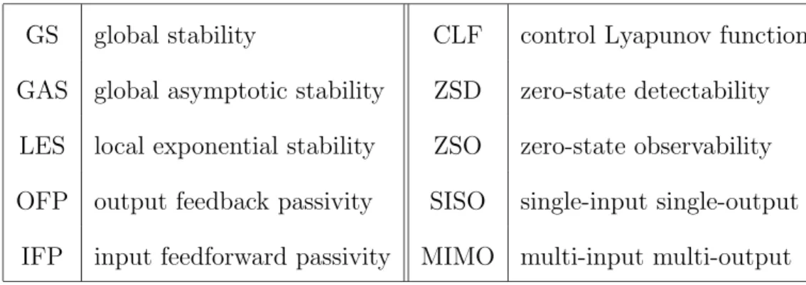
Table 1.1: List of acronyms.

GS global stability CLF control Lyapunov function

GAS global asymptotic stability ZSD zero-state detectability LES local exponential stability ZSO zero-state observability OFP output feedback passivity SISO single-input single-output

IFP input feedforward passivity MIMO multi-input multi-output

A C0 _{function β : IR}+_{× IR}+ _{→ IR}+ _{is said to belong to class} _{KL if for}

each fixed s the function β(·, s) belongs to class K, and for each fixed r, the function β(r,_{·) is decreasing and β(r, s) → 0 as s → ∞.}

For the reader’s convenience, Table 1.1 contains a list of acronyms used through-out the book.

(33)

Chapter 2 Passivity Concepts as Design

Tools

Only a few system theory concepts can match passivity in its physical and intuitive appeal. This explains the longevity of the passivity concept from the time of its first appearance some 60 years ago, to its current use as a tool for nonlinear feedback design. The pioneering results of Lurie and Popov, summarized in the monographs by Aizerman and Gantmacher [3], and Popov [88], were extended by Yakubovich [121], Kalman [51], Zames [123], Willems [120], and Hill and Moylan [37], among others. The first three sections of this chapter are based on these references from which we extract, and at times reformulate, the most important concepts and system properties to be used in the rest of the book.

We begin by defining and illustrating the concepts of storage function, supply rate, dissipativity and passivity in Section 2.1. The most useful aspect of these concepts, discussed in Section 2.2, is that they reveal the properties of parallel and feedback interconnections in which excess of passivity in one subsystem can compensate for the shortage in the other.

After these preparatory sections, we proceed to establish, in Section 2.3, the relationship between different forms of passivity and stability. Particularly important are the conditions for stability of feedback interconnections. In Section 2.4, we present a characterization of systems which can be rendered passive by feedback. The concept of feedback passive systems has evolved from recent work of Kokotovi´c and Sussmann [59], and Byrnes, Isidori, and Willems [15]. It is one of the main tools for our cascade and passivation designs.

(34)

2.1 Dissipativity and Passivity

2.1.1 Classes of systems

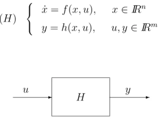
Although the passivity concepts apply to wider classes of systems, we restrict our attention to dynamical systems modeled by ordinary differential equations with an input vector u and an output vector y:

(H)    ˙x = f (x, u), x∈ IRn y = h(x, u), u, y ∈ IRm (2.1.1) - _H -u y

Figure 2.1: Input-output representation of (2.1.1).

We will be concerned with the case when the state x(t), as a function of time, is uniquely determined by its initial value x(0) and the input function u(t). We assume that u : IR+ _{→ IR}m _{belongs to an input set U of functions}

which are bounded on all bounded subintervals of IR+_{. In feedback designs}

u becomes a function of x, so the assumption u ∈ U cannot be a priori veri-fied. The satisfaction of this assumption for initial conditions in the region of interest will have to be a posteriori guaranteed by the design.

Another restriction in this chapter is that the system (2.1.1) is “square,” that is, its input and output have the same dimension m. Finally, an assump-tion made for convenience is that the system (2.1.1) has an equilibrium at the origin, that is, f (0, 0) = 0, and h(0, 0) = 0.

We will find it helpful to visualize the system (2.1.1) as the input-output block diagram in Figure 2.1. In such block diagrams the dependence on the initial state x(0) will not be explicitly stressed, but must not be overlooked.

The system description (2.1.1) includes as special cases the following three classes of systems:

• Nonlinear systems affine in the input:

˙x = f (x) + g(x)u

(35)

• Static nonlinearity:

y = ϕ(u) (2.1.3)

• Linear systems:

˙x = Ax + Bu

y = Cx + Du (2.1.4)

For static nonlinearity y = ϕ(u), the state space is void. In the case of linear systems, we will let the system H be represented by its transfer function H(s) := D + C(sI− A)−1_{B where s = σ + jω is the complex variable.}

2.1.2 Basic concepts

For an easy understanding of the concepts of dissipativity and passivity it is convenient to imagine that H is a physical system with the property that its energy can be increased only through the supply from an external source. From an abundance of real-life examples let us think of baking a potato in a microwave oven. As long as the potato is not allowed to burn, its energy can increase only as supplied by the oven. A similar observation can be made about an RLC-circuit connected to an external battery. The definitions given below are abstract generalizations of such physical properties.

Definition 2.1 (Dissipativity)

Assume that associated with the system H is a function w : IRm_{× IR}m _{→ IR,}

called the supply rate, which is locally integrable for every u _{∈ U, that is, it} satisfiesRt1

t0 |w(u(t), y(t))| dt < ∞ for all t0 ≤ t1. Let X be a connected subset

of IRn _{containing the origin. We say that the system H is dissipative in X}

with the supply rate w(u, y) if there exists a function S(x), S(0) = 0, such that for all x_{∈ X}

S(x)≥ 0 and S(x(T )) − S(x(0)) ≤

Z T

0 w(u(t), y(t)) dt (2.1.5)

for all u_{∈ U and all T ≥ 0 such that x(t) ∈ X for all t ∈ [0, T ]. The function}

S(x) is then called a storage function. 2

Definition 2.2 (Passivity)

System H is said to be passive if it is dissipative with supply rate w(u, y) =

uT_y. ₂

We see that passivity is dissipativity with bilinear supply rate. In our circuit example, the storage function S is the energy, w is the input power,

(36)

and R₀T w(u(t), y(t)) dt is the energy supplied to the system from the external sources. The system is dissipative if the increase in its energy during the interval (0, T ) is not bigger than the energy supplied to the system during that interval.

If the storage function S(x) is differentiable, we can write (2.1.5) as ˙

S(x(t)) _{≤ w(u(t), y(t))} (2.1.6)

Again, the interpretation is that the rate of increase of energy is not bigger than the input power.

If H is dissipative, we can associate with it a function Sa(x), called the

available storage, defined as Sa(x) = sup u,T ≥0 ( − Z T 0 w(u(t), y(t)) dt ¯ ¯ ¯ ¯ ¯x(0) = x and∀t ∈ [0, T ] : x(t) ∈ X ) (2.1.7) An interpretation of the available storage Sa(x) is that it is the largest amount

of energy which can be extracted from the system given the initial condition x(0) = x.

The available storage Sa(x) is itself a storage function and any other storage

function must satisfy S(x)≥ Sa(x). This can be seen by rewriting (2.1.5) as

S(x(0))_{≥ S(x(0)) − S(x(T )) ≥ −} Z T 0 w(u(t), y(t)) dt, which yields S(x(0))_{≥ sup} u,T ≥0 ( − Z T 0 w(u(t), y(t)) dt ) = Sa(x(0))

The properties of Sa(x) are summarized in the following theorem due to

Willems [120].

Theorem 2.3 (Available Storage)

The system H is dissipative in X with the supply rate w(u, y) if and only if Sa(x) is defined for all x∈ X. Moreover, Sa(x) is itself a storage function and,

if S(x) is another storage function with the same supply rate w(u, y), then

S(x)_{≥ S}a(x). 2

For linear passive systems, the available storage function is further char-acterized in the following theorem by Willems [120] which we quote without proof.

(37)

Theorem 2.4 (Quadratic storage function for linear systems)

If H is linear and passive, then the available storage function is quadratic Sa(x) = xTP x. The matrix P is the limit P = lim²→0P² of the real symmetric

positive semidefinite solution P² ≥ 0 of the Ricatti equation

P²A + ATP²+ (P²B− CT)(D + DT + ²I)−1(BTP²− CT) = 0

2 The above concepts are now illustrated with several examples.

Example 2.5 (Integrator as a passive system) An integrator is the simplest storage element:

˙x = u y = x

This system is passive with S(x) = 1₂x2 _{as a storage function because ˙}_{S = uy.}

Its available storage Sa can be obtained from the following inequalities:

1 2x 2 0 = S(x0)≥ Sa(x0) = sup u,T ( − Z T 0 yu dt ) ≥ Z _∞ 0 y 2_{dt = x}2 0 Z _∞ 0 e −2t_{dt =} 1 2x 2 0

The second inequality sign is obtained by choosing u =−y and T = ∞. Note that, for the choice u = _{−y, the assumption u ∈ U is a posteriori verified by} the fact that with this choice u(t) =−y(t) is a decaying exponential. 2 In most of our examples, the domain X of dissipativity will be the entire space IRn_{. However, for nonlinear systems, this is not always the case.}

Example 2.6 (Local passivity) The system

˙x = (x3_{− kx) + u}

y = x

is passive in the interval X = [₋√k,√k]_{⊂ IR with S(x) =} 1 2x

2 _{as a storage}

function because ˙S = x2_(x2_{− k) + uy ≤ uy for all x in X. However, we can}

verify that it is not passive in any larger subset of IRn_{: for any constant ¯}_k,

the input u = _−(¯k3 _{− k¯k) and the initial condition x = ¯k yield the constant}

solution x(t)≡ ¯k. If the system is passive, then along this solution, we must have 0 = S(x(T ))_{− S(x(0)) ≤} Z T 0 u(t)y(t) dt =−¯k 2_(¯_k2 − k)T

This is violated for ¯k _{6∈ [−}√k,√k], and hence, the system is not passive outside

Constructive Nonlinear Control

Preface

Contents

Chapter 1

Introduction

1.1

Passivity, Optimality, and Stability

1.1.1

From absolute stability to passivity

1.1.2

Passivity as a phase characteristic

1.1.3

Optimal control and stability margins

1.2

Feedback Passivation

1.2.1

Limitations of feedback linearization

1.2.2

Feedback passivation and forwarding

1.3

Cascade Designs

1.3.1

Passivation with composite Lyapunov functions

1.3.2

A structural obstacle: peaking

1.4

Lyapunov Constructions

1.4.1

Construction of the cross-term

1.4.2

A benchmark example

1.4.3

Adaptive control

1.5

Recursive Designs

1.5.1

Obstacles to passivation

1.5.2

Removing the relative degree obstacle

1.5.3

Removing the minimum phase obstacle

1.5.4

System structures

1.5.5

Approximate asymptotic designs

1.6

Book Style and Notation

1.6.1

Style

1.6.2

Notation and acronyms

Chapter 2

Passivity Concepts as Design

Tools

2.1

Dissipativity and Passivity

2.1.1

Classes of systems

2.1.2

Basic concepts